跳到论文正文
W Papers独立论文阅读器 arXiv:1106.1069 论文正文 计算阅读时间 · 0%
引用这篇论文根据当前论文元数据生成,正式投稿前建议核对。


License: arXiv.org perpetual non-exclusive license
arXiv:1106.1069v2 [hep-ph] 31 Oct 2011

ZAGREB-ZTF-11-04

Exotic Seesaw-Motivated Heavy Leptons at the LHC

Krešimir Kumerički, Ivica Picek and Branimir Radovčić

Department of Physics, Faculty of Science, University of Zagreb, P.O.B. 331, HR-10002 Zagreb, Croatia

August 24, 2026

PACS: 14.60.Hi; 14.60.Pq; 14.60.St
Keywords: Heavy leptons; Tree-level seesaw; Neutrino mass; Non-standard neutrinos

Abstract

We study the LHC potential for discovering TeV-scale S​U​(2)LSU(2)_{L} 5-plet fermions introduced recently to explain small neutrino masses. We show that the Drell-Yan production and the decays of new exotic Σ\Sigma leptons are testable at the LHC. Their production is abundant due to nontrivial electroweak gauge charges. For 1​fb−11\ \rm{fb^{-1}} of integrated luminosity at the present LHC s=7\sqrt{s}=7 TeV, there can be 270 Σ\Sigma-Σ¯\overline{\Sigma} pairs produced for MΣ=400​GeVM_{\Sigma}=\rm{400\ GeV}. Besides producing same-sign dilepton events, they could lead, due to a chosen small mixing between heavy and light leptons, to ∼\sim10 golden decays Σ+++(Σ+++¯)→W±W±l±\Sigma^{+++}(\overline{\Sigma^{+++}})\to W^{\pm}W^{\pm}l^{\pm} with a specific decay signature.

1 Introduction

The start-up of the Large Hadron Collider (LHC) has enabled the exploration of previously inaccessible domains of heavy particles, which are at the core of various extensions of the standard model (SM). A distinguished class of modifications of the particle content of the SM attributes the smallness of the masses of observed neutrinos to the presence of a seesaw mechanism. In such a setup the neutrino masses can be realized through an effective dimension-five operator L​L​H​HLLHH [1] which can be generated both at the tree and at the loop level. At the tree level there are three realizations of the dimension-five operator [2], all of them based on an addition of a single new multiplet: Type-I [3], type-II [4] and type-III [5] seesaw mechanisms, mediated by heavy fermion singlet, scalar triplet and a fermion triplet, respectively. Thereby, the fermionic type-I and III models involve hypercharge zero heavy Majorana mediators. Originally, the seesaw scale was linked to high energy GUT scale, while a recent reincarnation of S​U​(5)SU(5) GUT model which within the adjoint 24 representation contains both a singlet and hypercharge zero fermion triplet, providing a low scale hybrid type-I and III seesaw model [6]. In a multiple seesaw approach first put forward in [7] and later extended in [8], the involved additional fields and additional discrete symmetries are instrumental in bringing the seesaw mechanism to the TeV scale [9] accessible at the LHC.

In the recently proposed approach of [10], which we are scrutinizing here, the lowering of the seesaw scale has been achieved without use of discrete symmetries. By relying only on the gauge symmetry and the renormalizability of the SM, we arrived at novel seesaw mechanism supported by nonzero hypercharge fermions in higher isomultiplets.

Such a line of research follows from our examination [11] of the vectorlike top partner, which by a sort of Dirac seesaw mechanism increases the mass of the top [12]. We then extended our quark-sector study to the leptons, to explore a possible role of TeV-scale vectorlike Dirac fermions as seesaw mediators.

Indeed, the heaviness of the top quark and the lightness of the Higgs boson have been the landmarks for several extensions of the SM which rely on vectorlike rather than on sequential fourth generation fermions. We have observed that there are two options that such states, in conjunction with appropriate new scalar fields, act as seesaw mediators: via the triplet fermions already introduced in [13] and via the fermion 5-plet proposed in [10]. The dimension nine (dim 9) operator produced at the tree level in the latter case leads to the seesaw formula mν∼v6/ΛN​P5m_{\nu}\sim v^{6}/\Lambda_{NP}^{5}, which reproduces the empirical neutrino masses mν∼10−1m_{\nu}\sim 10^{-1} eV with sub-TeV 5-plet mass MΣM_{\Sigma}. This calls to investigate the phenomenology of new Dirac-type heavy leptons as the subject of our present study. Let us note that the focus of a study in Ref. [13] with their exotic nonzero hypercharge triplet fermions has been on the accompanied triply-charged scalars, whereas a more recent study [14] considered the effects of these triplet fermions on the LFV decays of charged SM leptons. In addition, some further constraints on exotic triplets have been placed very recently in Ref. [15, 16].

The present study of exotic 5-plet fermions can be compared to previous studies of hypercharge-zero triplets belonging to type-III seesaw mechanism: The earlier one performed by Franceschini et al. [17] and a subsequent by Li and He [18], which has some overlap with more recent study [19] of type-III triplets appearing also in already mentioned hybrid type-I and III seesaw model [6].

This article is organized as follows. In Section 2 we describe a tree-level seesaw model based on nonzero hypercharge fermions and point out the nonminimal (conjunct) appearance of exotic fermions and scalars needed for dim 7 and dim 9 seesaw mechanisms. Section 3 deals with the production rates, and Section 4 with the subsequent decays of exotic 5-plet states. We summarize our results in Section 5. The details on the mixing between light and heavy leptons are exposed in the Appendix.

2 TeV-scale seesaw model with higher isomultiplets

As a distinctive feature of the SM, the observed fundamental matter fields (quarks and leptons) are distributed in the lowest possible representations of the SM group, S​U​(3)C×S​U​(2)L×U​(1)YSU(3)_{C}\times SU(2)_{L}\times U(1)_{Y}. In addition to the leptonic left-handed doublets and the right-handed singlets, there is also the SM Higgs doublet, H=(H+,H0)TH=(H^{+},H^{0})^{T}. The values (2​T+1,Y)(2T+1,Y) of the weak isospin TT and hypercharge YY, indicated in the parentheses,

LL∼(2,−1),lR∼(1,−2),H∼(2,1),\displaystyle L_{L}\sim(2,-1),~~~l_{R}\sim(1,-2),~~~H\sim(2,1), (1)

reproduce the electric charges Q=T3+Y/2Q=T_{3}+Y/2 of the respective multiplet components.

Higher, isotriplet multiplets ∼(3,2)\sim(3,2) and ∼(3,0)\sim(3,0) are already familiar from type-II and III seesaw models, and it is obvious that we may encounter a 5-plet of zero hypercharge as the simplest generalization of type-III seesaw Majorana triplet to a higher-isospin multiplet. Incidentally, such a ∼(5,0)\sim(5,0) fermion multiplet has been singled out in the literature as a viable minimal dark matter (MDM) candidate [20]. It provides a completely neutral (T3=0T_{3}=0 and Y=0Y=0) component of an additional S​U​(2)LSU(2)_{L} multiplet, and the minimality refers to its isolated appearance: MDM is realized as a single additional exotic matter particle coupled to the SM fields.
However, our concern here is with the seesaw models where exotic fermionic seesaw mediators appear together with appropriate exotic scalar isomultiplets. Thereby, in order to add something new to already existing seesaw mechanisms, we employ vectorlike fermionic multiplets with nonzero hypercharge. In contrast to chiral SM fermions, the masses of such vectorlike fermions are not restricted to the electroweak scale, so that they can be naturally adjusted to the new physics scale. If in a novel seesaw mechanism the new physics appears already around the TeV scale, then this scenario would not suffer from an additional, seesaw-induced hierarchy problem. In order to produce a tree-level seesaw, the newly introduced fermion multiplets have to have a neutral component which will mix with light neutrinos. Accompanying new scalar multiplets also have to have a neutral component which can acquire the vacuum expectation value (vev). As exposed to more detail in the next subsection, these requirements together with the SM gauge symmetry lead to rather restricted viable quantum number assignments for the new multiplets: the one with vectorlike triplet fermions introduced in [13] leading to dim 7 seesaw operator, and the vectorlike fermion 5-plet introduced by [10] leading to dim 9 seesaw operator.

2.1 Dim 9 seesaw model with fermionic 5-plets

The effective operators of the form (L​L​H​H)​(H†​H)n(LLHH)(H^{\dagger}H)^{n} have already been studied in [21, 22], and more recently in [23], where it has been pointed out that the mass operator at each higher dimension is unique, independent of the mechanism leading to it.

The model pursued here starts from three generations of SM model leptons represented by LLL_{L} and lRl_{R} in Eq. (1) and adds to them nΣn_{\Sigma} isospin T=2T=2 vectorlike 5-plets of leptons with hypercharge two, where both left and right components transform as (5,2)(5,2) under the electroweak part of the SM group,

ΣL,R=(Σ+++Σ+⁣+Σ+Σ0Σ−)L,R∼(5,2).\displaystyle\Sigma_{L,R}=\left(\begin{array}[]{l}\Sigma^{+++}\\ \Sigma^{++}\\ \Sigma^{+}\\ \Sigma^{0}\\ \Sigma^{-}\end{array}\right)_{L,R}\sim~~(5,2)~~.

Besides the SM Higgs doublet HH in Eq. (1) there are two additional isospin T=3/2T=3/2 scalar multiplets Φ1\Phi_{1} and Φ2\Phi_{2} transforming as (4,−3)(4,-3) and (4,−1)(4,-1), respectively:

Φ1=(ϕ10ϕ1−ϕ1−⁣−ϕ1−−−)∼(4,−3),Φ2=(ϕ2+ϕ20ϕ2−ϕ2−⁣−)∼(4,−1).\displaystyle\Phi_{1}=\left(\begin{array}[]{l}\phi_{1}^{0}\\ \phi_{1}^{-}\\ \phi_{1}^{--}\\ \phi_{1}^{---}\end{array}\right)\sim~~(4,-3),~~~\Phi_{2}=\left(\begin{array}[]{l}\phi_{2}^{+}\\ \phi_{2}^{0}\\ \phi_{2}^{-}\\ \phi_{2}^{--}\end{array}\right)\sim~~(4,-1).~

Explaining the neutrino masses by dim 9 operator leads to the exotic matter shown in Eqs. (2.1) and (2.1). Concerning the fermion fields Σ\Sigma, they should be vectorlike in order to avoid the chiral anomaly. The extra scalar fields are constrained by a requirement of the renormalizability of the extended SM, restricting the Lagrangian of the scalar sector to dimension 4 terms. Accordingly, the weak isospin of the exotic scalar fields (Φ1,2\Phi_{1,2}) can not be higher than three half, in order that they couple linearly with the Higgs field and develop an induced vev after the spontaneous symmetry breaking of the SM gauge group. For this reason, the scalar fields should be in multiplets which contain electrically neutral components.

Seesaw Type Exotic Fermion Exotic Scalar Scalar Coupling mνm_{\nu} at
Type-I NR∼(1,0)N_{R}\sim(1,0) - - dim 5
Type-II - Δ∼(3,2)\Delta\sim(3,2) μ​Δ​H​H\mu\Delta HH dim 5
Type-III NR∼(3,0)N_{R}\sim(3,0) - - dim 5
Conjunct Exotic Fermion Exotic Scalars Scalar - Higgs mνm_{\nu} at
Mediator Pair Φ1,Φ2\Phi_{1},\ \Phi_{2} Couplings
doublet ΣL,R​(2,1)\Sigma_{L,R}\ (2,1) (3,−2),(3,0)(3,-2),\ (3,0) μ1,2​Φ1,2​H​H\mu_{1,2}\Phi_{1,2}HH dim 5
triplet ΣL,R​(3,2)\Sigma_{L,R}\ (3,2) (4,−3),(2,−1)(4,-3),\ (2,-1) λ1​Φ1​H​H​H\lambda_{1}\Phi_{1}HHH dim 7
4-plet ΣL,R​(4,1)\Sigma_{L,R}\ (4,1) (3,−2),(3,0)(3,-2),\ (3,0) μ1,2​Φ1,2​H​H\mu_{1,2}\Phi_{1,2}HH dim 5
5-plet ΣL,R​(5,2)\Sigma_{L,R}\ (5,2) (4,−3),(4,−1)(4,-3),\ (4,-1) λ1,2​Φ1,2​H​H​H\lambda_{1,2}\Phi_{1,2}HHH dim 9
Table 1: The assignments of electroweak charges for exotic particles leading to the tree-level seesaw operator up to dim 9.

Since the sought-after dim 9 operator can be relevant only in the absence of possible dim 5 operators, we forbid the appearance of those states which generate conventional seesaw mechanisms. In first place, we should avoid a scalar triplet Δ∼(3,2)\Delta\sim(3,2) generating type-II seesaw, and a fermion singlet NR∼(1,0)N_{R}\sim(1,0) or triplet NR∼(3,0)N_{R}\sim(3,0) generating type-I and III seesaw, respectively (see the Table 1). Note that type-I, II, and III mechanisms correspond to already mentioned minimal (single) appearance of exotic (EX) scalar/fermionic particles in the Yukawa term

ℒYminimal∼(SM-fermion) (SM-scalar/fermion) (EX-fermion/scalar).\mathcal{L}_{Y}^{\text{minimal}}\sim\text{(SM-fermion) (SM-scalar/fermion) (EX-fermion/scalar)}. (17)

Also, a recent study of exotic triplets in Ref. [15, 16] restricts to such minimal Yukawa term. We generalize Eq. (17) to new Yukawa terms with double appearance of exotic particles,

ℒYconjunct∼(SM-fermion) (EX-scalar) (EX-fermion),\mathcal{L}_{Y}^{\text{conjunct}}\sim\text{(SM-fermion) (EX-scalar) (EX-fermion)}\ , (18)

where a conjunct exotic scalar-fermion pair can lead to the neutrino mass operators of dimension larger then 5, as shown in Table 1.

Consequently, the focus here is on nonzero hypercharge Dirac fermions ΣL,R\Sigma_{L,R} from the last row of Table 1, playing role of the seesaw mediators which produce the mechanism displayed on Fig. 1. The seesaw diagram on this figure arises due to the Yukawa couplings explicated in Eq. (19) and the scalar-field couplings λ1\lambda_{1} and λ2\lambda_{2} explicated in Eq. (38). Note that it involves a decomposition of the appropriate couplings in terms of the Clebsch-Gordan coefficients.

Refer to caption
Figure 1: Dim 9 tree-level seesaw diagram produced by exotic fields in Eqs. (2.1) and (2.1).

In order to avoid already known seesaw mechanisms, there is a gap between the quantum numbers of the SM fields and the EX fields. To overbridge this gap and to obtain the gauge invariant interaction in Eq. (18), the conjunct EX scalar-fermion pair should form an object with the weak isospin half and the hypercharge one. One possible way to achieve this is shown in the doublet and 4-plet “Seesaw Type“ rows in Table 1, where new fermion fields of isospin one half (doublet) or three half (4-plet) hold together with a scalar of isospin one (triplet). However the latter appears already in type-II seesaw and would lead to dim 5 operator for neutrino masses. Then we are left with new fermion fields which should be of either isospin one (triplet) or isospin two (5-plet). Whereas the first option corresponds to dim 7 operator introduced by Babu et al. [13], we adopt the latter case corresponding to dim 9 operator which might be more accessible for tests at the LHC. The requirement of employing the Dirac fermions as tree-level seesaw mediators restricts their hypercharge to Y=2Y=2 for both the triplet and the 5-plet case.

2.2 Mass matrices of the 5-plet states

For our choice of EX fields in Eqs. (2.1) and (2.1) the conjunct Yukawa interaction in Eq. (18) is explicated by the second row in the following gauge invariant Lagrangian:

ℒ\displaystyle\mathcal{L} =\displaystyle= ΣL¯​i​D​ΣL+ΣR¯​i​D​ΣR−ΣR¯​MΣ​ΣL−ΣL¯​MΣ†​ΣR\displaystyle\overline{\Sigma_{L}}i\cancel{D}\Sigma_{L}+\overline{\Sigma_{R}}i\cancel{D}\Sigma_{R}-\overline{\Sigma_{R}}M_{\Sigma}\Sigma_{L}-\overline{\Sigma_{L}}M_{\Sigma}^{\dagger}\Sigma_{R} (19)
+\displaystyle+ (ΣR¯Y1LLΦ1∗+(ΣL)c¯Y2LLΦ2+H.c.).\displaystyle\left(\overline{\Sigma_{R}}Y_{1}L_{L}\Phi_{1}^{*}+\overline{(\Sigma_{L})^{c}}Y_{2}L_{L}\Phi_{2}+\mathrm{H.c.}\right)\ .

This contains the bare Dirac mass terms for the introduced vectorlike lepton 5-plet fields

−ℒD=\displaystyle-\mathcal{L}_{D}= ΣR+++¯MΣΣL++++ΣR+⁣+¯MΣΣL+⁣+\displaystyle\overline{\Sigma_{R}^{+++}}M_{\Sigma}\Sigma_{L}^{+++}+\overline{\Sigma_{R}^{++}}M_{\Sigma}\Sigma_{L}^{++} (20)
+ΣR+¯​MΣ​ΣL++ΣR0¯​MΣ​ΣL0+ΣR−¯​MΣ​ΣL−+H.c..\displaystyle+\overline{\Sigma_{R}^{+}}M_{\Sigma}\Sigma_{L}^{+}+\overline{\Sigma_{R}^{0}}M_{\Sigma}\Sigma_{L}^{0}+\overline{\Sigma_{R}^{-}}M_{\Sigma}\Sigma_{L}^{-}+\mathrm{H.c.}\ .

Additional mass terms arise from the Yukawa part in Eq. (19). As discussed shortly, an analysis of the scalar potential shows that the neutral components of two scalar quadruplets Φ10\Phi^{0}_{1} and Φ20\Phi^{0}_{2} develop the induced vevs, vΦ1v_{\Phi_{1}} and vΦ2v_{\Phi_{2}}, respectively. This means that Yukawa terms in Eq. (19) lead to the mass terms connecting the SM lepton doublet with new vectorlike lepton 5-plet. Thereby, the triply and doubly charged states do not mix with SM leptons whereas the singly-charged and neutral states have peculiar mixing with SM leptons which we consider in detail in the Appendix.

When extracting the mass matrices produced by the mass and Yukawa terms we suppress the generation indices of the fields. Three neutral left-handed fields νL\nu_{L}, ΣL0\Sigma_{L}^{0} and (ΣR0)c(\Sigma_{R}^{0})^{c} span the symmetric neutral mass matrix as follows:

ℒν​Σ0=−12​((νL)c¯​(ΣL0)c¯​ΣR0¯)​(0m2Tm1Tm20MΣTm1MΣ0)​(νLΣL0(ΣR0)c)+H.c..\displaystyle\mathcal{L}_{\nu\Sigma^{0}}=\,-\frac{1}{2}\left(\overline{(\nu_{L})^{c}}\;\overline{(\Sigma_{L}^{0})^{c}}\;\overline{\Sigma_{R}^{0}}\right)\left(\!\begin{array}[]{ccc}0&m_{2}^{T}&m_{1}^{T}\\ m_{2}&0&M_{\Sigma}^{T}\\ m_{1}&M_{\Sigma}&0\end{array}\!\right)\,\left(\!\!\begin{array}[]{c}\nu_{L}\\ \Sigma_{L}^{0}\\ (\Sigma_{R}^{0})^{c}\end{array}\!\!\right)\;+\mathrm{H.c.}\ .

For singly-charged fermions we arrive at the nonsymmetric mass matrix which explicates the mixing between the SM leptons and new singly-charged states

ℒl​Σ=−(lR¯​ΣR−¯​(ΣL+)c¯)​(ml00m3MΣ0m40MΣT)​(lLΣL−(ΣR+)c)+H.c..\displaystyle\mathcal{L}_{l\Sigma}=\,-\left(\overline{l_{R}}\;\overline{\Sigma_{R}^{-}}\;\overline{(\Sigma_{L}^{+})^{c}}\right)\left(\!\begin{array}[]{ccc}m_{l}&0&0\\ m_{3}&M_{\Sigma}&0\\ m_{4}&0&M_{\Sigma}^{T}\end{array}\!\right)\,\left(\!\!\begin{array}[]{c}l_{L}\\ \Sigma_{L}^{-}\\ (\Sigma_{R}^{+})^{c}\end{array}\!\!\right)\;+\mathrm{H.c.}\ .

Here MΣM_{\Sigma} is given in Eq. (20), while m3m_{3} and m4m_{4} entries in Eq. (2.2) and m1m_{1} and m2m_{2} in the neutral sector in Eq. (2.2) come from the respective terms in Eq. (19):

m1=110​Y1​vΦ∗1,\displaystyle m_{1}=\sqrt{\frac{1}{10}}Y_{1}{v^{*}_{\Phi}}_{1}\ , m2=−320​Y2​vΦ2,\displaystyle\qquad m_{2}=-\sqrt{\frac{3}{20}}Y_{2}{v_{\Phi}}_{2}\ ,
m3=25​Y1​vΦ∗1,\displaystyle m_{3}=\sqrt{\frac{2}{5}}Y_{1}{v^{*}_{\Phi}}_{1}\ , m4=110​Y2​vΦ2.\displaystyle\qquad m_{4}=\sqrt{\frac{1}{10}}Y_{2}{v_{\Phi}}_{2}\ . (35)

Accordingly, the masses mim_{i} (i=1,2,3,4i=1,2,3,4) are determined by the vev vΦ1v_{\Phi_{1}} and vev vΦ2v_{\Phi_{2}} of the neutral components of the scalar quadruplets, whereas MΣM_{\Sigma} is on the new physics scale ΛN​P\Lambda_{NP}, which is larger than the electroweak scale.

The diagonalization of the mass matrices proceeds by unitary transformations presented in the Appendix. They are the result of a procedure developed in Ref. [24], whereby we write the leading order expressions up to MΣ−2M^{-2}_{\Sigma} in the basis where the matrices mlm_{l} and MΣM_{\Sigma} are already diagonalized. Block diagonalization of the neutral mass matrix in Eq. (2.2) gives to this order

m~ν≃−m2T​MΣ−1​m1−m1T​MΣ−1​m2,\tilde{m}_{\nu}\simeq-m_{2}^{T}M^{-1}_{\Sigma}m_{1}-m_{1}^{T}M^{-1}_{\Sigma}m_{2}\ , (36)

where a familiar unitary V​(3×3)P​M​N​SV(3\times 3)_{PMNS} matrix diagonalizes the obtained effective light neutrino mass matrix:

VP​M​N​ST​m~ν​VP​M​N​S=mν.V_{PMNS}^{T}\tilde{m}_{\nu}V_{PMNS}=m_{\nu}\ . (37)

The same formalism has been applied in Refs. [18, 25] and the results in our Appendix agree with theirs, when taking the appropriate limits.

2.3 Dim 9 w.r.t. dim 5 loop-level seesaw mechanisms

Turning to the scalar potential, we restrict ourselves to already mentioned renormalizable terms, relevant for our mechanism:

V⁡(H,Φ1,Φ2)\displaystyle V(H,\Phi_{1},\Phi_{2}) ∼\displaystyle\sim μH2​H†​H+μΦ12​Φ1†​Φ1+μΦ22​Φ2†​Φ2+λH​(H†​H)2\displaystyle\mu_{H}^{2}H^{\dagger}H+\mu^{2}_{\Phi_{1}}\Phi^{\dagger}_{1}\Phi_{1}+\mu^{2}_{\Phi_{2}}\Phi^{\dagger}_{2}\Phi_{2}+\lambda_{H}(H^{\dagger}H)^{2} (38)
+\displaystyle+ {λ1Φ1∗H∗H∗H∗+H.c.}+{λ2Φ2∗HH∗H∗+H.c.}\displaystyle\{\lambda_{1}\Phi^{*}_{1}H^{*}H^{*}H^{*}+\mathrm{H.c.}\}+\{\lambda_{2}\Phi^{*}_{2}HH^{*}H^{*}+\mathrm{H.c.}\}
+\displaystyle+ {λ3Φ1∗Φ2H∗H∗+H.c.}.\displaystyle\{\lambda_{3}\Phi^{*}_{1}\Phi_{2}H^{*}H^{*}+\mathrm{H.c.}\}\ .

The electroweak symmetry breaking proceeds in the usual way from the vev v=174​GeVv=174\ \rm{GeV} of the Higgs doublet, implying μH2<0\mu_{H}^{2}<0. On the other hand, the electroweak ρ\rho parameter dictates the vevs vΦ1v_{\Phi_{1}} and vΦ2v_{\Phi_{2}} to be small, implying μΦ12,μΦ22>0\mu^{2}_{\Phi_{1}},\mu^{2}_{\Phi_{2}}>0. However, the λ1\lambda_{1} and λ2\lambda_{2} terms in Eq. (38) result in the induced vevs for the isospin 3/2 scalar multiplets,

vΦ1≃−λ1​v3μΦ12,vΦ2≃−λ2​v3μΦ22.v_{\Phi_{1}}\simeq-\lambda_{1}\frac{v^{3}}{\mu^{2}_{\Phi_{1}}}\,\,,\,\,v_{\Phi_{2}}\simeq-\lambda_{2}\frac{v^{3}}{\mu^{2}_{\Phi_{2}}}\,\,. (39)

Let us stress that we allow only the SM scalar doublet to wear a Mexican hat, and that the terms linear in the extra scalar fields, which induce their vevs, only slightly deform the total scalar potential without affecting the vev of the SM Higgs. Generically, the potential in Eq. (38) is at large field values dominated by the terms quartic in fields, and with a number of free parameters in the potential there is no problem to ensure the stability of the SM vacuum.

The nonanishing vevs in Eq. (39) change the electroweak ρ\rho parameter to ρ⁡(Φ1)≃1−6​vΦ12/v2\rho(\Phi_{1})\simeq 1-6v^{2}_{\Phi_{1}}/v^{2} and ρ⁡(Φ2)≃1+6​vΦ22/v2\rho(\Phi_{2})\simeq 1+6v^{2}_{\Phi_{2}}/v^{2}, respectively. If these vevs are taken separately, the experimental value ρ=1.0000−0.0007+0.0011\rho=1.0000^{+0.0011}_{-0.0007} [26] leads to the upper bounds vΦ1≤1.9v_{\Phi_{1}}\leq 1.9 GeV and vΦ2≤2.4v_{\Phi_{2}}\leq 2.4 GeV, respectively. Thus, the value of a few GeV can be considered as an upper bound on both vΦ1v_{\Phi_{1}} and vΦ2v_{\Phi_{2}} if there is no fine-tuning between them. By merging Eqs. (35),  (36) and  (39) we obtain for the light neutrino mass

mν∼Y1​Y2​λ1​λ2​v6MΣ​μΦ12​μΦ22,m_{\nu}\sim\frac{Y_{1}Y_{2}\ \lambda_{1}\lambda_{2}\ v^{6}}{M_{\Sigma}\ \mu^{2}_{\Phi_{1}}\ \mu^{2}_{\Phi_{2}}}\,, (40)

which leads to dim 9 seesaw formula result, mν∼v6/ΛN​P5m_{\nu}\sim v^{6}/\Lambda_{NP}^{5}.

Neutrino masses can arise from dim 5 operators generated at the loop level. The loop factors provide a sufficient suppression as exploited by one- [27], two- [28, 29] and three-loop level [30] mechanisms. Such a loop level generated dim 5 operator arises also in our extension of the SM. As explained in [10], there is a restricted range of the parameter space where the dim 5 loop-contributions shown on Fig. 2 are smaller than the dim 9 tree-level contribution shown on Fig. 1. With an extra assumption on the scalar field coupling strengths in (38), λ3≃λ1⋅λ2\lambda_{3}\simeq\lambda_{1}\cdot\lambda_{2}, the dim 9 mechanism turns out to be the leading one for ΛN​P∼\Lambda_{NP}\sim few 100 GeV. The loop contributions prevail for ΛN​P∼\Lambda_{NP}\sim several TeV, which are beyond the direct reach of the LHC, and may also mark a virtual physics in the LHC era.
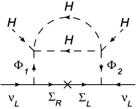
Refer to caption
Refer to caption
Figure 2: Dim 5 operator arising at the loop level: the two-loop seesaw diagram given by the λ1\lambda_{1} and λ2\lambda_{2} couplings in Eq. (38), and the one-loop seesaw diagram given by the λ3\lambda_{3} coupling in Eq. (38).

3 Production of 5-plet leptons at the LHC

The production channels of the heavy 5-plet leptons in proton-(anti)proton collisions are dominated by the quark-antiquark annihilation via neutral and charged gauge bosons

q+q¯→A→Σ+Σ¯,A=γ,Z,W±,q+\bar{q}\to A\to\Sigma+\bar{\Sigma}\;,\qquad A=\gamma,Z,W^{\pm}\;,

where the gauge Lagrangian relevant for the production

ℒg​a​u​g​eΣ​Σ¯=\displaystyle\mathcal{L}_{gauge}^{\Sigma\overline{\Sigma}}= +\displaystyle+ e(3Σ+++¯γμΣ++++2Σ+⁣+¯γμΣ+⁣++Σ+¯γμΣ+−Σ−¯γμΣ−)Aμ\displaystyle e(3\overline{\Sigma^{+++}}\gamma^{\mu}\Sigma^{+++}+2\overline{\Sigma^{++}}\gamma^{\mu}\Sigma^{++}+\overline{\Sigma^{+}}\gamma^{\mu}\Sigma^{+}-\overline{\Sigma^{-}}\gamma^{\mu}\Sigma^{-})A_{\mu} (41)
+\displaystyle+ gcW((2−3sW2)Σ+++¯γμΣ++++(1−2sW2)Σ+⁣+¯γμΣ+⁣+)Zμ\displaystyle{g\over c_{W}}((2-3s_{W}^{2})\overline{\Sigma^{+++}}\gamma^{\mu}\Sigma^{+++}+(1-2s_{W}^{2})\overline{\Sigma^{++}}\gamma^{\mu}\Sigma^{++})Z_{\mu}
+\displaystyle+ gcW​((−sW2)​Σ+¯​γμ​Σ++(−1)​Σ0¯​γμ​Σ0+(−2+sW2)​Σ−¯​γμ​Σ−)​Zμ\displaystyle{g\over c_{W}}((-s_{W}^{2})\overline{\Sigma^{+}}\gamma^{\mu}\Sigma^{+}+(-1)\overline{\Sigma^{0}}\gamma^{\mu}\Sigma^{0}+(-2+s_{W}^{2})\overline{\Sigma^{-}}\gamma^{\mu}\Sigma^{-})Z_{\mu}
+\displaystyle+ g(2Σ+⁣+¯γμΣ++++3Σ+¯γμΣ+⁣++3Σ0¯γμΣ++2Σ−¯γμΣ0)Wμ−+H.c.\displaystyle g(\sqrt{2}\overline{\Sigma^{++}}\gamma^{\mu}\Sigma^{+++}+\sqrt{3}\overline{\Sigma^{+}}\gamma^{\mu}\Sigma^{++}+\sqrt{3}\overline{\Sigma^{0}}\gamma^{\mu}\Sigma^{+}+\sqrt{2}\overline{\Sigma^{-}}\gamma^{\mu}\Sigma^{0})W^{-}_{\mu}+\mathrm{H.c.}

is contained in Eq. (123) in the Appendix. The cross section for the partonic process is determined entirely by gauge couplings and is given by

σ^​(q​q¯→Σ​Σ¯)=β⁡(3−β2)48​π​s^​(VL2+VR2),\hat{\sigma}(q\bar{q}\to\Sigma\overline{\Sigma})=\frac{\beta(3-\beta^{2})}{48\pi}\hat{s}(V_{L}^{2}+V_{R}^{2})\;, (42)

where s^≡(pq+pq¯)2\hat{s}\equiv(p_{q}+p_{\bar{q}})^{2} is the Mandelstam variable ss for the quark-antiquark system, the parameter β≡1−4​MΣ2/s^\beta\equiv\sqrt{1-4M_{\Sigma}^{2}/\hat{s}} denotes the heavy lepton velocity, and the left- and right-handed couplings in Eq. (42) are given by

VL,R(γ+Z)\displaystyle V_{L,R}^{(\gamma+Z)} =QΣ​Qq​e2s^+gZ​Σ​gL,Rq​g2cW2​(s^−MZ2),\displaystyle=\frac{Q_{\Sigma}Q_{q}e^{2}}{\hat{s}}+\frac{g^{Z\Sigma}\,g_{L,R}^{q}\,g^{2}}{c_{W}^{2}(\hat{s}-M_{Z}^{2})}\;, (43)
VL(W−)\displaystyle V_{L}^{(W^{-})} =gW​Σ​g2​Vu​d2​(s^−MW2)=VL(W+)∗,\displaystyle=\frac{g^{W\Sigma}g^{2}V_{ud}}{\sqrt{2}(\hat{s}-M_{W}^{2})}=V_{L}^{(W^{+})^{*}}\;, (44)
VR(W±)\displaystyle V_{R}^{(W^{\pm})} =0.\displaystyle=0\;. (45)

Here, gLq=T3−sW2​Qqg^{q}_{L}=T_{3}-s_{W}^{2}Q_{q} and gRq=−sW2​Qqg^{q}_{R}=-s_{W}^{2}Q_{q} are the SM chiral quark couplings to the ZZ boson. The vector couplings of heavy leptons to gauge bosons are

gZ​Σ=T3−sW2QΣ,gW​Σ=2,3,3and2,g^{Z\Sigma}=T_{3}-s_{W}^{2}Q_{\Sigma}\ ,\ g^{W\Sigma}=\sqrt{2},\sqrt{3},\sqrt{3}\ \rm{and}\ \sqrt{2}\ , (46)

where gW​Σg^{W\Sigma} can be read of the last raw in Eq. (41) relevant for the production of Σ+++Σ+⁣+¯\Sigma^{+++}\overline{\Sigma^{++}}, Σ+⁣+​Σ+¯\Sigma^{++}\overline{\Sigma^{+}}, Σ+​Σ0¯\Sigma^{+}\overline{\Sigma^{0}} and Σ0​Σ−¯\Sigma^{0}\overline{\Sigma^{-}} pairs, respectively. We note, in passing, that the choices gZ​Σ=cW2g^{Z\Sigma}=c_{W}^{2} and gW​Σ=1g^{W\Sigma}=1, appropriate for the type-III seesaw model, reproduce the expressions given in [17].

Refer to caption
Figure 3: The cross sections for production of 5-plet lepton pairs on LHC proton-proton collisions at s=7​TeV\sqrt{s}=7\,{\rm TeV} via neutral γ,Z\gamma,Z (a) and charged W±W^{\pm} currents (b), in dependence on the heavy 5-plet mass MM.

To obtain the cross sections for a hadron collider, the partonic cross-section (42) has to be convoluted with the appropriate parton distribution functions (PDF) q⁡(x,μ2)q(x,\mu^{2}). For the case of the proton-proton collisions we have

d2​σ​(p​p→Σ​Σ¯)d​x1​d​x2=1Nc​∑f1=u,d,…∑f2=u¯,d¯,…σ^​(qf1​qf2→Σ​Σ¯)×(qf1​(x1,μ2)​qf2​(x2,μ2)+qf2​(x1,μ2)​qf1​(x2,μ2)),\frac{d^{2}\sigma(pp\to\Sigma\overline{\Sigma})}{dx_{1}dx_{2}}=\frac{1}{N_{c}}\sum_{f_{1}=u,d,\dots}\sum_{f_{2}=\bar{u},\bar{d},\dots}\>\hat{\sigma}(q_{f_{1}}{q}_{f_{2}}\to\Sigma\overline{\Sigma})\\ \times\big(q_{f_{1}}(x_{1},\mu^{2})q_{f_{2}}(x_{2},\mu^{2})+q_{f_{2}}(x_{1},\mu^{2})q_{f_{1}}(x_{2},\mu^{2})\big)\;, (47)

leading to the total cross section

σ⁡(p​p→Σ​Σ¯)=1Nc​∑f1=u,d,…∑f2=u¯,d¯,…∫4​M2/s1d​τ​∫τ1d​x1x1​σ^​(qf1​qf2→Σ​Σ¯)×(qf1​(x1,μ2)​qf2​(τx1,μ2)+qf2​(x1,μ2)​qf1​(τx1,μ2)).\sigma(pp\to\Sigma\overline{\Sigma})=\frac{1}{N_{c}}\sum_{f_{1}=u,d,\dots}\sum_{f_{2}=\bar{u},\bar{d},\dots}\int_{4M^{2}/s}^{1}d\tau\,\int_{\tau}^{1}\frac{dx_{1}}{x_{1}}\>\hat{\sigma}(q_{f_{1}}{q}_{f_{2}}\to\Sigma\overline{\Sigma})\\ \times\Big(q_{f_{1}}(x_{1},\mu^{2})q_{f_{2}}(\frac{\tau}{x_{1}},\mu^{2})+q_{f_{2}}(x_{1},\mu^{2})q_{f_{1}}(\frac{\tau}{x_{1}},\mu^{2})\Big)\;. (48)

Here, the inverse of the Nc=3N_{c}=3 factor is due to the color averaging in the initial state, corresponding to the summation over colors implicit in the standard published PDF functions. To evaluate the cross sections we have used CTEQ6.6 PDFs [31] via LHAPDF software library [32] and have chosen μ=MΣ\mu=M_{\Sigma} as a factorization scale. Comparison with other PDF sets has shown that uncertainty in cross sections induced by the choice of PDFs is less than 3%. We find an excellent agreement when checking our calculations with an independent evaluation of cross sections performed by using MadGraph [33], where the present model has been implemented with the help of FeynRules package [34].

The cross sections for proton-proton collisions are presented at s=7​TeV\sqrt{s}=7\,{\rm TeV}, appropriate for the current LHC run, on Fig. 3, and for designed s=14​TeV\sqrt{s}=14\,{\rm TeV} on Fig. 4. On Fig. 5 cross sections for proton-antiproton collisions, relevant for the Tevatron at s=1.96​TeV\sqrt{s}=1.96\,{\rm TeV} are presented. Thereby we distinguish separately the production via neutral currents shown on LHS, and via charged currents shown on RHS of Figs. 3 to 5.

Refer to caption
Figure 4: Same as Fig. 3, but for designed s=14​TeV\sqrt{s}=14\,{\rm TeV} at the LHC.
Refer to caption
Figure 5: Same as Fig. 3, but for s=1.96​TeV\sqrt{s}=1.96\,{\rm TeV} at the Tevatron.
Produced Cross section (fb\rm{fb})
pair MΣ=200​GeVM_{\Sigma}=200\ \rm{GeV} MΣ=400​GeVM_{\Sigma}=400\ \rm{GeV} MΣ=800​GeVM_{\Sigma}=800\ \rm{GeV}
Σ+++Σ+++¯\Sigma^{+++}\overline{\Sigma^{+++}} 967 36.6 0.47
Σ+⁣+​Σ+⁣+¯\Sigma^{++}\overline{\Sigma^{++}} 267 10.3 0.13
Σ+​Σ+¯\Sigma^{+}\overline{\Sigma^{+}} 29 1.1 0.02
Σ0​Σ0¯\Sigma^{0}\overline{\Sigma^{0}} 253 9.3 0.11
Σ−​Σ−¯\Sigma^{-}\overline{\Sigma^{-}} 939 34.6 0.43
Σ+++Σ+⁣+¯\Sigma^{+++}\overline{\Sigma^{++}} 641 26.5 0.32
Σ+⁣+​Σ+¯\Sigma^{++}\overline{\Sigma^{+}} 961 39.8 0.49
Σ+​Σ0¯\Sigma^{+}\overline{\Sigma^{0}} 961 39.8 0.49
Σ0​Σ−¯\Sigma^{0}\overline{\Sigma^{-}} 641 26.5 0.32
Σ+⁣+​Σ+++¯\Sigma^{++}\overline{\Sigma^{+++}} 276 9.1 0.10
Σ+​Σ+⁣+¯\Sigma^{+}\overline{\Sigma^{++}} 414 13.6 0.16
Σ0​Σ+¯\Sigma^{0}\overline{\Sigma^{+}} 414 13.6 0.16
Σ−​Σ0¯\Sigma^{-}\overline{\Sigma^{0}} 276 9.1 0.10
Total 7040 269.9 3.30
Table 2: Production cross sections for Σ\Sigma-Σ¯\overline{\Sigma} pairs for the current LHC run at s=7​TeV\sqrt{s}=7\,{\rm TeV}, for three selected values of MΣM_{\Sigma}.

We extract the pair production cross sections shown in Fig. 3 for three selected values of MΣM_{\Sigma} which we show in Table 2. From this table we find that the triply-charged Σ+++\Sigma^{+++} has the biggest production cross section σ(Σ+++)|MΣ=400​G​e​V=63.1fb\sigma(\Sigma^{+++})|_{M_{\Sigma}=400\rm{GeV}}=63.1\,\rm{fb} and singly-charged Σ−\Sigma^{-} has the smallest, but comparable, production cross section σ⁡(Σ−)|MΣ=400​G​e​V=43.7​fb\sigma(\Sigma^{-})|_{M_{\Sigma}=400\rm{GeV}}=43.7\,\rm{fb}. Production cross sections for all other particles and antiparticles from a 5-plet are in between. In particular, for 1​fb−11\ \rm{fb^{-1}} of integrated luminosity at the present LHC s=7\sqrt{s}=7 TeV, there would be 270 Σ\Sigma-Σ¯\overline{\Sigma} pairs in total produced for MΣ=400​GeVM_{\Sigma}=400\,\rm{GeV}, among which are ∼100\sim 100 triply-charged Σ+++\Sigma^{+++} or Σ+++¯\overline{\Sigma^{+++}} fermions. Note that the production at the LHC and Tevatron, which is comparable in the case of light Σ\Sigma-states, changes dramatically in favor of the LHC for higher values of the Σ\Sigma-lepton masses. Therefore, only the restricted mass region is covered on Fig. 5 for the Tevatron.

By testing the heavy lepton production cross sections one can hope to identify the quantum numbers of the 5-plet particles, but in order to confirm their relation to neutrinos one has to study their decays.

4 Decays of 5-plet states

Provided that in our scenario the exotic scalar states in Eq. (2.1) are slightly heavier than the exotic leptons in Eq. (2.1), the exotic scalars will not appear in the final states in heavy lepton decays. Also, the most phenomenologically interesting triply-charged scalar state is common to our model and the model by Babu et al. [13] where it has been in the focus of their study, so that there is no need to repeat their study here. Thus we focus entirely on the decay modes of the heavy lepton states in Eq. (2.1). Let us note that the ordering of the states in this formula corresponds to the spectrum of these states, running from the lightest Σ−\Sigma^{-} to the heaviest Σ+++\Sigma^{+++} state.

The mass difference induced by loops of SM gauge bosons between two components of Σ\Sigma 5-plet with electric charges QQ and Q′Q^{\prime} is explicitly calculated in [20]

MQ−MQ′=\displaystyle M_{Q}-M_{Q^{\prime}}= α2​M4​π{(Q2−Q′2)sW2f(MZM)+(Q−Q′)(Q+Q′−Y)\displaystyle\frac{\alpha_{2}M}{4\pi}\Big\{(Q^{2}-Q^{\prime 2})s_{\rm W}^{2}f(\frac{M_{Z}}{M})+(Q-Q^{\prime})(Q+Q^{\prime}-Y) (49)
[f(MWM)−f(MZM)]},\displaystyle\bigg[f(\frac{M_{W}}{M})-f(\frac{M_{Z}}{M})\bigg]\Big\}\ ,

where

f⁡(r)=r2​[2​r3​ln⁡r−2​r+(r2−4)1/2​(r2+2)​ln⁡(r2−2−r​r2−42)].f(r)={r\over 2}\left[2r^{3}\ln r-2r+(r^{2}-4)^{1/2}(r^{2}+2)\ln\left({r^{2}-2-r\sqrt{r^{2}-4}\over 2}\right)\right]\ . (50)

For MΣ=400​GeVM_{\Sigma}=400\ \rm{GeV} we get

MΣ+++−MΣ+⁣+≃1130MeV,MΣ+⁣+−MΣ+≃804MeV,\displaystyle M_{\Sigma^{+++}}-M_{\Sigma^{++}}\simeq 1130\ \rm{MeV},\ M_{\Sigma^{++}}-M_{\Sigma^{+}}\simeq 804\ \rm{MeV},
MΣ+−MΣ0≃477​MeV,MΣ0−MΣ−≃150​MeV.\displaystyle M_{\Sigma^{+}}-M_{\Sigma^{0}}\simeq 477\ \rm{MeV},\ M_{\Sigma^{0}}-M_{\Sigma^{-}}\simeq 150\ \rm{MeV}\ . (51)

The neutral Σ0\Sigma^{0} and singly-charged Σ+\Sigma^{+} states, coming in Eq. (51), receive additional corrections given in Eqs. (5) and (122), respectively. However, being of the order of magnitude of the light neutrino masses, these corrections are completely negligible.

The splitting ∼1\sim 1 GeV between triply and doubly charged 5-plet states opens additional decay channels, in particular, the ρ\rho resonance enhanced decay channel to the two pions in the final state.

4.1 Pointlike MΣM_{\Sigma}-dependent decays

The Lagrangian in the mass-eigenstate basis relevant for the decays of the heavy leptons is the result of a detailed calculation exposed in the Appendix. Let us repeat here the neutral and charged current terms,

ℒN​C​Z\displaystyle\mathcal{L}_{NCZ} =\displaystyle= gcW[ν¯(32VP​M​N​S†V1γμPL−32​2VP​M​N​STV2∗γμPR)Σ0\displaystyle{g\over c_{W}}\Big[\overline{\nu}({3\over 2}V_{PMNS}^{\dagger}V_{1}\gamma^{\mu}P_{L}-{\sqrt{3}\over 2\sqrt{2}}V_{PMNS}^{T}V^{*}_{2}\gamma^{\mu}P_{R})\Sigma^{0} (52)
+\displaystyle+ l¯(3V1γμPL)Σ−+lc¯(12V2∗γμPR)Σ+]Zμ0+H.c.,\displaystyle\overline{l}(3V_{1}\gamma^{\mu}P_{L})\Sigma^{-}+\overline{l^{c}}({1\over 2}V^{*}_{2}\gamma^{\mu}P_{R})\Sigma^{+}\Big]Z_{\mu}^{0}+\mathrm{H.c.}\ ,

and

ℒC​C\displaystyle\mathcal{L}_{CC} =\displaystyle= g[ν¯(−3VP​M​N​S†V1γμPL+2VP​M​N​STV2∗γμPR)Σ+\displaystyle g\Big[\overline{\nu}(-\sqrt{3}V_{PMNS}^{\dagger}V_{1}\gamma^{\mu}P_{L}+\sqrt{2}V_{PMNS}^{T}V^{*}_{2}\gamma^{\mu}P_{R})\Sigma^{+} (53)
+\displaystyle+ Σ−¯​(3​V2T​VP​M​N​S∗​γμ​PR)​ν+l¯​(−32​V1​γμ​PL)​Σ0\displaystyle\overline{\Sigma^{-}}(\sqrt{3}V^{T}_{2}V_{PMNS}^{*}\gamma^{\mu}P_{R})\nu+\overline{l}(-{3\over\sqrt{2}}V_{1}\gamma^{\mu}P_{L})\Sigma^{0}
+\displaystyle+ Σ0¯(−32V2TγμPR)lc+lc¯(−3V2∗γμPR)Σ+⁣+]Wμ−+H.c.\displaystyle\overline{\Sigma^{0}}(-{\sqrt{3}\over 2}V^{T}_{2}\gamma^{\mu}P_{R})l^{c}+\overline{l^{c}}(-\sqrt{3}V^{*}_{2}\gamma^{\mu}P_{R})\Sigma^{++}\Big]W_{\mu}^{-}+\mathrm{H.c.}\

Here, all the couplings can be expressed in terms of the matrix-valued quantities V1V_{1} and V2V_{2} explicated in the Appendix, corresponding to the mass matrices in Eq. (35)

V1=110​Y1†​vΦ1​MΣ−1,V2=110​Y2†​vΦ∗2​MΣ−1.V_{1}=\sqrt{\frac{1}{10}}Y^{\dagger}_{1}{v_{\Phi}}_{1}M^{-1}_{\Sigma}\ ,V_{2}=\sqrt{\frac{1}{10}}Y^{\dagger}_{2}{v^{*}_{\Phi}}_{2}M^{-1}_{\Sigma}\ . (54)

Out of the five Σ\Sigma-states in Eq. (2.1), the four lying lowest have the pointlike decays to the gauge bosons and SM leptons. Here, in contrast to type-III triplet states, the decays of 5-plet states into the SM Higgs boson are suppressed. When appropriate, we will comment on further differences with respect to the decays of type-III triplet states.

Let us start our list of the partial decay widths by the decays of neutral Σ0\Sigma^{0} state:

Γ⁡(Σ0→ℓ−​W+)=g232​π​|32​V1ℓ​Σ|2​MΣ3MW2​(1−MW2MΣ2)2​(1+2​MW2MΣ2),\displaystyle\Gamma(\Sigma^{0}\to\ell^{-}W^{+})={g^{2}\over 32\pi}\Big|{3\over\sqrt{2}}V_{1}^{\ell\Sigma}\Big|^{2}{M_{\Sigma}^{3}\over M_{W}^{2}}\left(1-{M_{W}^{2}\over M_{\Sigma}^{2}}\right)^{2}\left(1+2{M_{W}^{2}\over M_{\Sigma}^{2}}\right),
Γ⁡(Σ0→ℓ+​W−)=g232​π​|32​V2ℓ​Σ|2​MΣ3MW2​(1−MW2MΣ2)2​(1+2​MW2MΣ2),\displaystyle\Gamma(\Sigma^{0}\to\ell^{+}W^{-})={g^{2}\over 32\pi}\Big|{\sqrt{3}\over 2}V_{2}^{\ell\Sigma}\Big|^{2}{M_{\Sigma}^{3}\over M_{W}^{2}}\left(1-{M_{W}^{2}\over M_{\Sigma}^{2}}\right)^{2}\left(1+2{M_{W}^{2}\over M_{\Sigma}^{2}}\right),
∑m=13Γ⁡(Σ0→νm​Z0)=g232​π​cW2​∑ℓ={e,μ,τ}(|32​V1ℓ​Σ|2+|32​2​V2ℓ​Σ|2)\displaystyle\sum^{3}_{m=1}\Gamma(\Sigma^{0}\to\nu_{m}Z^{0})={g^{2}\over 32\pi c_{W}^{2}}\sum_{\ell=\{e,\mu,\tau\}}\Big(\Big|{3\over 2}V_{1}^{\ell\Sigma}\Big|^{2}+\Big|{\sqrt{3}\over 2\sqrt{2}}V_{2}^{\ell\Sigma}\Big|^{2}\Big)
MΣ3MZ2​(1−MZ2MΣ2)2​(1+2​MZ2MΣ2).\displaystyle{M_{\Sigma}^{3}\over M_{Z}^{2}}\left(1-{M_{Z}^{2}\over M_{\Sigma}^{2}}\right)^{2}\left(1+2{M_{Z}^{2}\over M_{\Sigma}^{2}}\right). (55)

These three decays, for two chosen set of couplings V1V_{1} and V2V_{2}, are displayed on Figs. 6 and 7 as a counterpart of Fig. 2 in Ref. [17] for type-III triplets. Thereby, the product of V1V_{1} and V2V_{2} is constrained by Eq. (36). Decays of Σ0\Sigma^{0} to leptons (antileptons) are governed by V1V_{1} (V2V_{2}), so that the branching ratios to leptons or antileptons are strongly dependent on the hierarchy between V1V_{1} and V2V_{2}, as illustrated in Figs. 6 and 7.

Refer to caption
Figure 6: Partial decay widths of Σ0\Sigma^{0} 5-plet lepton for |V1l​Σ|=|V2l​Σ|=10−6​20MΣ​(GeV)|V^{l\Sigma}_{1}|=|V^{l\Sigma}_{2}|=10^{-6}\sqrt{{20\over M_{\Sigma}\rm{(GeV)}}}, in dependence on heavy 5-plet mass MΣM_{\Sigma}.
Refer to caption
Figure 7: Partial decay widths of Σ0\Sigma^{0} 5-plet lepton for |V1l​Σ|=10−6​0.5MΣ​(GeV)|V^{l\Sigma}_{1}|=10^{-6}\sqrt{{0.5\over M_{\Sigma}\rm{(GeV)}}} different from |V2l​Σ|=10−6​800MΣ​(GeV)|V^{l\Sigma}_{2}|=10^{-6}\sqrt{{800\over M_{\Sigma}\rm{(GeV)}}}, in dependence on heavy 5-plet mass MΣM_{\Sigma}.

Besides the representative Σ0\Sigma^{0} decays above, let us present also the rest of the pointlike decays. For a negative singly-charged heavy lepton Σ−\Sigma^{-} the partial decay widths are given by:

Γ⁡(Σ−→ℓ−​Z0)=g232​π​cW2​|3​V1ℓ​Σ|2​MΣ3MZ2​(1−MZ2MΣ2)2​(1+2​MZ2MΣ2),\displaystyle\Gamma(\Sigma^{-}\to\ell^{-}Z^{0})={g^{2}\over 32\pi c_{W}^{2}}\Big|3V_{1}^{\ell\Sigma}\Big|^{2}{M_{\Sigma}^{3}\over M_{Z}^{2}}\left(1-{M_{Z}^{2}\over M_{\Sigma}^{2}}\right)^{2}\left(1+2{M_{Z}^{2}\over M_{\Sigma}^{2}}\right),
∑m=13Γ⁡(Σ−→νm​W−)=g232​π​∑ℓ={e,μ,τ}|3​V2ℓ​Σ|2\displaystyle\sum^{3}_{m=1}\Gamma(\Sigma^{-}\to\nu_{m}W^{-})={g^{2}\over 32\pi}\sum_{\ell=\{e,\mu,\tau\}}\Big|\sqrt{3}V_{2}^{\ell\Sigma}\Big|^{2}
MΣ3MW2​(1−MW2MΣ2)2​(1+2​MW2MΣ2).\displaystyle{M_{\Sigma}^{3}\over M_{W}^{2}}\left(1-{M_{W}^{2}\over M_{\Sigma}^{2}}\right)^{2}\left(1+2{M_{W}^{2}\over M_{\Sigma}^{2}}\right). (56)

The positive singly-charged Σ+\Sigma^{+} state has the following partial decay widths:

Γ⁡(Σ+→ℓ+​Z0)=g232​π​cW2​|12​V2ℓ​Σ|2​MΣ3MZ2​(1−MZ2MΣ2)2​(1+2​MZ2MΣ2),\displaystyle\Gamma(\Sigma^{+}\to\ell^{+}Z^{0})={g^{2}\over 32\pi c_{W}^{2}}\Big|{1\over 2}V_{2}^{\ell\Sigma}\Big|^{2}{M_{\Sigma}^{3}\over M_{Z}^{2}}\left(1-{M_{Z}^{2}\over M_{\Sigma}^{2}}\right)^{2}\left(1+2{M_{Z}^{2}\over M_{\Sigma}^{2}}\right),
∑m=13Γ⁡(Σ+→νm​W+)=g232​π​∑ℓ={e,μ,τ}(|3​V1ℓ​Σ|2+|2​V2ℓ​Σ|2)\displaystyle\sum^{3}_{m=1}\Gamma(\Sigma^{+}\to\nu_{m}W^{+})={g^{2}\over 32\pi}\sum_{\ell=\{e,\mu,\tau\}}\Big(\Big|\sqrt{3}V_{1}^{\ell\Sigma}\Big|^{2}+\Big|\sqrt{2}V_{2}^{\ell\Sigma}\Big|^{2}\Big)
MΣ3MW2​(1−MW2MΣ2)2​(1+2​MW2MΣ2).\displaystyle{M_{\Sigma}^{3}\over M_{W}^{2}}\left(1-{M_{W}^{2}\over M_{\Sigma}^{2}}\right)^{2}\left(1+2{M_{W}^{2}\over M_{\Sigma}^{2}}\right). (57)

Finally, the doubly-charged Σ+⁣+\Sigma^{++} state decays exclusively via a charged current, with the partial decay width

Γ⁡(Σ+⁣+→ℓ+​W+)=g232​π​|3​V2ℓ​Σ|2​MΣ3MW2​(1−MW2MΣ2)2​(1+2​MW2MΣ2).\Gamma(\Sigma^{++}\to\ell^{+}W^{+})={g^{2}\over 32\pi}\Big|\sqrt{3}V_{2}^{\ell\Sigma}\Big|^{2}{M_{\Sigma}^{3}\over M_{W}^{2}}\left(1-{M_{W}^{2}\over M_{\Sigma}^{2}}\right)^{2}\left(1+2{M_{W}^{2}\over M_{\Sigma}^{2}}\right). (58)

Let us stress that there is no such pointlike decay for the triply-charged Σ+++\Sigma^{+++}. This state, instead, has some other interesting decays studied in the next subsections.

Σ+¯→ℓ−​Z0\overline{\Sigma^{+}}\to\ell^{-}Z^{0} Σ0¯→ℓ+​W−\overline{\Sigma^{0}}\to\ell^{+}W^{-} Σ0¯→ℓ−​W+\overline{\Sigma^{0}}\to\ell^{-}W^{+} Σ−¯→ℓ+​Z0\overline{\Sigma^{-}}\to\ell^{+}Z^{0}
Σ+→ℓ+​Z0\Sigma^{+}\to\ell^{+}Z^{0} ℓ+​ℓ−​Z0​Z0\ell^{+}\ell^{-}Z^{0}Z^{0} ℓ+​ℓ+​Z0​W−\ell^{+}\ell^{+}Z^{0}W^{-} ℓ+​ℓ−​Z0​W+\ell^{+}\ell^{-}Z^{0}W^{+} -
Σ0→ℓ−​W+\Sigma^{0}\to\ell^{-}W^{+} ℓ−​ℓ−​W+​Z0\ell^{-}\ell^{-}W^{+}Z^{0} ℓ−​ℓ+​W+​W−\ell^{-}\ell^{+}W^{+}W^{-} ℓ−​ℓ−​W+​W+\ell^{-}\ell^{-}W^{+}W^{+} ℓ−​ℓ+​W+​Z0\ell^{-}\ell^{+}W^{+}Z^{0}
Σ0→ℓ+​W−\Sigma^{0}\to\ell^{+}W^{-} ℓ+​ℓ−​W−​Z0\ell^{+}\ell^{-}W^{-}Z^{0} ℓ+​ℓ+​W−​W−\ell^{+}\ell^{+}W^{-}W^{-} ℓ+​ℓ−​W−​W+\ell^{+}\ell^{-}W^{-}W^{+} ℓ+​ℓ+​W−​Z0\ell^{+}\ell^{+}W^{-}Z^{0}
Σ−→ℓ−​Z0\Sigma^{-}\to\ell^{-}Z^{0} - ℓ−​ℓ+​Z0​W−\ell^{-}\ell^{+}Z^{0}W^{-} ℓ−​ℓ−​Z0​W+\ell^{-}\ell^{-}Z^{0}W^{+} ℓ−​ℓ+​Z0​Z0\ell^{-}\ell^{+}Z^{0}Z^{0}
Table 3: Decays of exotic leptons to SM particles including same sign dilepton events

In Table 3 we list all possible events coming from the decays of the neutral and singly-charged 5-plet states to the SM charged leptons. This includes the same-sign dilepton events as a distinguished signature at the LHC.

4.2 Decays which do not depend on any free parameter

Besides previous decays, there are also decays of Σi\Sigma^{i} to a lighter Σj\Sigma^{j} state. The decay rate for a single pion finale state is given by

Γ⁡(Σi→Σj​π+)=(gW​Σ)i​j2​2π​GF2​|Vu​d|2​fπ2​(Δ​Mi​j)3​1−mπ2(Δ​Mi​j)2.\Gamma(\Sigma^{i}\to\Sigma^{j}\pi^{+})=(g^{W\Sigma})^{2}_{ij}{2\over\pi}G_{\rm F}^{2}|V_{ud}|^{2}f_{\pi}^{2}(\Delta M_{ij})^{3}\sqrt{1-\frac{m_{\pi}^{2}}{(\Delta M_{ij})^{2}}}\ . (59)

The corresponding leptonic decay is

Γ⁡(Σi→Σj​l+​ν)=(gW​Σ)i​j2​215​π3​GF2​(Δ​Mi​j)5​1−ml2(Δ​Mi​j)2\Gamma(\Sigma^{i}\to\Sigma^{j}l^{+}\nu)=(g^{W\Sigma})^{2}_{ij}{2\over 15\pi^{3}}G_{\rm F}^{2}(\Delta M_{ij})^{5}\sqrt{1-\frac{m_{l}^{2}}{(\Delta M_{ij})^{2}}} (60)

where (gW​Σ)i​j2(g^{W\Sigma})^{2}_{ij} is given in Eq. (46) and Δ​Mi​j=Mi−Mj\Delta M_{ij}=M_{i}-M_{j} is given in Eq. (49).

Such decays are suppressed by small mass differences, except for Σ+++\Sigma^{+++} where the mass difference Δ​M32\Delta M_{32} between the Σ+++\Sigma^{+++} and Σ+⁣+\Sigma^{++} state is large enough to enable also the two pions in the final state. This three-body decay is dominated by a ρ⁡(770)\rho(770) resonance, and we obtain for it an analytical formula expressed in terms of the meson decay constants, fπ≃f_{\pi}\simeq 130 MeV and fρ≃f_{\rho}\simeq 150 MeV,

Γ(Σ+++→Σ+⁣+π+π0)≃Γ(Σ+++→Σ+⁣+ρ+)=\displaystyle\Gamma(\Sigma^{+++}\to\Sigma^{++}\pi^{+}\pi^{0})\simeq\Gamma(\Sigma^{+++}\to\Sigma^{++}\rho^{+})=
24π​GF2​Vu​d2​fρ2​(Δ​M32)3​(1−4​mπ2mρ2)−1​1−mρ2(Δ​M32)2.\displaystyle{24\over\pi}G_{\rm F}^{2}V_{ud}^{2}f_{\rho}^{2}(\Delta M_{32})^{3}\Big(1-\frac{4m_{\pi}^{2}}{m_{\rho}^{2}}\Big)^{-1}\sqrt{1-\frac{m_{\rho}^{2}}{(\Delta M_{32})^{2}}}\ . (61)

This decay shows an enhancement with respect to the corresponding two-body decay

Γ(Σ+++→Σ+⁣+π+π0)Γ(Σ+++→Σ+⁣+π+)=6​fρ2fπ2​1−mρ2(Δ​M32)21−mπ2(Δ​M32)2​(1−4​mπ2mρ2)−1.{\Gamma(\Sigma^{+++}\to\Sigma^{++}\pi^{+}\pi^{0})\over\Gamma(\Sigma^{+++}\to\Sigma^{++}\pi^{+})}=6{f_{\rho}^{2}\over f_{\pi}^{2}}{\sqrt{1-\frac{m_{\rho}^{2}}{(\Delta M_{32})^{2}}}\over\sqrt{1-\frac{m_{\pi}^{2}}{(\Delta M_{32})^{2}}}}\Big(1-\frac{4m_{\pi}^{2}}{m_{\rho}^{2}}\Big)^{-1}\ . (62)

These decays will serve as the referent decays for the golden decay mode of the triply-charged state studied in the following subsection.

4.3 Golden Σ+++→W+W+l+\Sigma^{+++}\to W^{+}W^{+}l^{+} decay

We now turn to evaluation of the decay rate for Σ+++→W+W+l+\Sigma^{+++}\to W^{+}W^{+}l^{+} with on-shell WW bosons.

Refer to caption
Figure 8: Feynman diagram contributing to the triply-charged golden decay

The Feynman diagram on Fig. 8 and its crossed, contribute with an off-shell Σ+⁣+\Sigma^{++} in the intermediate state.

The expression for the amplitude squared is lengthy so we give the analytical expression for decay width only in the limit MΣ≫MWM_{\Sigma}\gg M_{W}:

Γ(Σ+++→W+W+l+)|MΣ≫MW=g2384​π2​sW2|3V2ℓ​Σ|2MΣ5MW4.\Gamma(\Sigma^{+++}\to W^{+}W^{+}l^{+})\big|_{M_{\Sigma}\gg M_{W}}={g^{2}\over 384\pi^{2}s_{W}^{2}}\Big|\sqrt{3}V_{2}^{\ell\Sigma}\Big|^{2}{M_{\Sigma}^{5}\over M_{W}^{4}}\ . (63)
Refer to caption
Figure 9: Selected partial decay widths of Σ+++\Sigma^{+++} 5-plet lepton for |V2l​Σ|=10−6​20MΣ​(GeV)|V^{l\Sigma}_{2}|=10^{-6}\sqrt{{20\over M_{\Sigma}\rm{(GeV)}}} in dependence of heavy 5-plet mass MΣM_{\Sigma}.
Refer to caption
Figure 10: Selected partial decay widths of Σ+++\Sigma^{+++} 5-plet lepton for |V2l​Σ|=10−6​800MΣ​(GeV)|V^{l\Sigma}_{2}|=10^{-6}\sqrt{{800\over M_{\Sigma}\rm{(GeV)}}} in dependence of heavy 5-plet mass MΣM_{\Sigma}.

Obviously, this decay is governed by the same mixing factor as in Σ+⁣+\Sigma^{++} decay in Eq. (58). Full numerical calculation, using FormCalc package [35], results in a partial width plotted on Figs. 9 and 10 for same choices of the mixing factor V2V_{2} as on previous figures. On the same figures we plot the partial widths of the decays of Σ+++\Sigma^{+++} given in Eqs. (59)-(61).

For the sake of being definite, let us explicate the branching ratios for the choice of heavy-light mixing V2V_{2} taken on Fig. 10, for two values of heavy-lepton mass MΣM_{\Sigma}

∑lBR(Σ+++→W+W+l+))|MΣ=400​G​e​V\displaystyle\sum_{l}BR(\Sigma^{+++}\to W^{+}W^{+}l^{+}))\Big|_{M_{\Sigma}=400\rm{GeV}} =\displaystyle= 0.09\displaystyle 0.09
∑lBR(Σ+++→W+W+l+))|MΣ=800​G​e​V\displaystyle\sum_{l}BR(\Sigma^{+++}\to W^{+}W^{+}l^{+}))\Big|_{M_{\Sigma}=800\rm{GeV}} =\displaystyle= 0.80.\displaystyle 0.80\ . (64)

As stated before, for 1​fb−11\ \rm{fb^{-1}} of integrated luminosity expected to be collected from the present LHC run at s=7\sqrt{s}=7 TeV, there will be ∼100\sim 100 triply-charged Σ+++\Sigma^{+++} or Σ+++¯\overline{\Sigma^{+++}} fermions produced. This will result in ∼\sim10 decays Σ+++(Σ+++¯)→W±W±l±\Sigma^{+++}(\overline{\Sigma^{+++}})\to W^{\pm}W^{\pm}l^{\pm} for MΣ=400​GeVM_{\Sigma}=400\ \rm{GeV} and |V2l​Σ|=10−6​800MΣ​(GeV)|V^{l\Sigma}_{2}|=10^{-6}\sqrt{{800\ \over M_{\Sigma}\rm{(GeV)}}}.

5 Conclusions

We have investigated the testability of exotic heavy leptons introduced to explain small neutrino masses. It is conceivable that such states additional to the SM leptons may appear as higher representations such as isospin 2 heavy fermions in conjunction with isospin 3/2 heavy scalar fields studied here. The LHC could provide enough energy and luminosity to produce and study such heavy particles if they mediate the proposed seesaw mechanism. In particular, the decays of new heavy leptons to SM particles depend on how light and heavy leptons mix with each other. Our seesaw model constrains the mixing to be small, given by the square root of the ratio of light and small masses, (mν/MΣ)1/2(m_{\nu}/M_{\Sigma})^{1/2}. This suppresses their effects on the flavor physics, but the abundant production of new states invites us to investigate the phenomenology of these heavy leptons at the LHC.

For 1​fb−11\ \rm{fb^{-1}} of integrated luminosity, the present LHC (s=7\sqrt{s}=7 TeV) run can produce in total 270 (7000) Σ\Sigma-Σ¯\overline{\Sigma} pairs of heavy leptons with mass MΣ=400​GeV​(200​GeV)M_{\Sigma}=\rm{400\ GeV\ (200\ GeV)}, among which there would be ∼100​(2850)\sim 100\ (2850) triply-charged Σ+++\Sigma^{+++} or Σ+++¯\overline{\Sigma^{+++}} fermions. Thereby, the triply-charged Σ+++\Sigma^{+++} has the biggest production cross-section, σ(Σ+++)|MΣ=400​G​e​V=63.1fb\sigma(\Sigma^{+++})|_{M_{\Sigma}=400\rm{GeV}}=63.1\ \rm{fb}, and singly-charged Σ−\Sigma^{-} has the smallest but still comparable σ⁡(Σ−)|MΣ=400​G​e​V=43.7​fb\sigma(\Sigma^{-})|_{M_{\Sigma}=400\rm{GeV}}=43.7\ \rm{fb}. The production cross-sections for all other particles and antiparticles from a 5-plet are in between. Notably, the production of triply-charged leptons is followed with its golden decays Σ+++(Σ+++¯)→W±W±l±\Sigma^{+++}(\overline{\Sigma^{+++}})\to W^{\pm}W^{\pm}l^{\pm}. For a chosen mass MΣ=400​GeVM_{\Sigma}=400\ \rm{GeV} and the mixing |V2l​Σ|=10−6​800MΣ​(GeV)|V^{l\Sigma}_{2}|=10^{-6}\sqrt{{800\ \over M_{\Sigma}\rm{(GeV)}}} we expect ∼\sim10 golden mode events.

The great advantage of the processes considered in this paper, common to most seesaw-inspired models, is the copious production of energetic leptons, which provides a clear experimental signature and relatively small SM background. Detailed studies of standard seesaw scenarios [36] demonstrate that final states with 2 (same sign) and 3 or 4 charged leptons can be increasingly easily distinguished from the SM background. For the model at hand, similar results are expected. For example, our prominent production channel pp¯→Σ+++Σ+++¯p\bar{p}\to\Sigma^{+++}\overline{\Sigma^{+++}} results in 3 or more energetic charged leptons in roughly one third of cases. Additionally, when it is experimentally possible to separate final-state particles coming from each of the two produced heavy leptons, then the three same-sign leptons coming from a single heavy-lepton lead to distinctive signature of the presented model. The corresponding SM background is essentially negligible, similarly to what has been demonstrated in [37] in generic new physics scenario with lepton number violation.

To conclude, the exotic 5-plet leptons introduced to explain small neutrino masses can be observed at LHC. At the designed LHC luminosity and s=14\sqrt{s}=14 TeV our 5-plet tree level seesaw model is falsifiable for sub-TeV Σ\Sigma-lepton masses, while for masses which are outside of the LHC reach the 5-plet leptons remain viable for generating radiative neutrino masses. In this sense, we hope that the involved predictive and testable vectorlike fermion 5-plet may establish an exciting link between collider phenomenology and the origin of neutrino masses.

Acknowledgements

We thank Borut Bajc, Walter Grimus and Goran Senjanović for discussions at the early stage of this research. K.K. and I.P. thank Jan O. Eeg for discussions and hospitality offered at the University in Oslo. This work is supported by the Croatian Ministry of Science, Education, and Sports under Contract No. 119-0982930-1016.

APPENDIX: The interaction vertices of the 5-plet

The novel seesaw model employs, in addition to the SM particles, nΣn_{\Sigma} vectorlike 5-plets of leptons with hypercharge two, ΣL,R∼(1,5,2)\Sigma_{L,R}\sim(1,5,2) under S​U​(3)C×S​U​(2)L×U​(1)YSU(3)_{C}\times SU(2)_{L}\times U(1)_{Y}. We write the component fields as

ΣL=(ΣL+++ΣL+⁣+ΣL+ΣL0ΣL−),ΣR=(ΣR+++ΣR+⁣+ΣR+ΣR0ΣR−).\displaystyle\Sigma_{L}=\left(\begin{array}[]{c}\Sigma_{L}^{+++}\\ \Sigma_{L}^{++}\\ \Sigma_{L}^{+}\\ \Sigma_{L}^{0}\\ \Sigma_{L}^{-}\\ \end{array}\right)\ \ \ ,\ \ \ \Sigma_{R}=\left(\begin{array}[]{c}\Sigma_{R}^{+++}\\ \Sigma_{R}^{++}\\ \Sigma_{R}^{+}\\ \Sigma_{R}^{0}\\ \Sigma_{R}^{-}\\ \end{array}\right)\ .

The renormalizable Lagrangian involving ΣL\Sigma_{L} and ΣR\Sigma_{R} is given by

ℒ\displaystyle\mathcal{L} =\displaystyle= ΣL¯​i​D​ΣL+ΣR¯​i​D​ΣR−ΣR¯​MΣ​ΣL−ΣL¯​MΣ†​ΣR\displaystyle\overline{\Sigma_{L}}i\cancel{D}\Sigma_{L}+\overline{\Sigma_{R}}i\cancel{D}\Sigma_{R}-\overline{\Sigma_{R}}M_{\Sigma}\Sigma_{L}-\overline{\Sigma_{L}}M_{\Sigma}^{\dagger}\Sigma_{R} (76)
+\displaystyle+ ΣR¯​Y1​LL​Φ1∗+(ΣL)c¯​Y2​LL​Φ2+H.c..\displaystyle\overline{\Sigma_{R}}Y_{1}L_{L}\Phi_{1}^{*}+\overline{(\Sigma_{L})^{c}}Y_{2}L_{L}\Phi_{2}+\mathrm{H.c.}\ .

With a nonzero vacuum expectation value for the scalar fields, doublet leptons receive mass and mix with the 5-plet leptons. Lepton mass terms in the Lagrangian are

ℒm\displaystyle\mathcal{L}_{m} =\displaystyle= −12​((νL)c¯​(ΣL0)c¯​ΣR0¯)​(0m2Tm1Tm20MΣTm1MΣ0)​(νLΣL0(ΣR0)c)+H.c.\displaystyle-\frac{1}{2}\left(\overline{(\nu_{L})^{c}}\;\overline{(\Sigma_{L}^{0})^{c}}\;\overline{\Sigma_{R}^{0}}\right)\left(\!\begin{array}[]{ccc}0&m_{2}^{T}&m_{1}^{T}\\ m_{2}&0&M_{\Sigma}^{T}\\ m_{1}&M_{\Sigma}&0\end{array}\!\right)\,\left(\!\!\begin{array}[]{c}\nu_{L}\\ \Sigma_{L}^{0}\\ (\Sigma_{R}^{0})^{c}\end{array}\!\!\right)\;+\mathrm{H.c.} (91)
−\displaystyle- (lR¯​ΣR−¯​(ΣL+)c¯)​(ml00m3MΣ0m40MΣT)​(lLΣL−(ΣR+)c)+H.c.\displaystyle\left(\overline{l_{R}}\;\overline{\Sigma_{R}^{-}}\;\overline{(\Sigma_{L}^{+})^{c}}\right)\left(\!\begin{array}[]{ccc}m_{l}&0&0\\ m_{3}&M_{\Sigma}&0\\ m_{4}&0&M_{\Sigma}^{T}\end{array}\!\right)\,\left(\!\!\begin{array}[]{c}l_{L}\\ \Sigma_{L}^{-}\\ (\Sigma_{R}^{+})^{c}\end{array}\!\!\right)\;+\mathrm{H.c.}
−\displaystyle- ΣR+⁣+¯MΣΣL+⁣+−ΣR+++¯MΣΣL++++H.c.,\displaystyle\overline{\Sigma_{R}^{++}}M_{\Sigma}\Sigma_{L}^{++}-\overline{\Sigma_{R}^{+++}}M_{\Sigma}\Sigma_{L}^{+++}+\mathrm{H.c.}\ ,

with

m1=110​Y1​vΦ∗1,\displaystyle m_{1}=\sqrt{\frac{1}{10}}Y_{1}{v^{*}_{\Phi}}_{1}\ , m2=−320​Y2​vΦ2,\displaystyle m_{2}=-\sqrt{\frac{3}{20}}Y_{2}{v_{\Phi}}_{2}\ ,
m3=25​Y1​vΦ∗1,\displaystyle m_{3}=\sqrt{\frac{2}{5}}Y_{1}{v^{*}_{\Phi}}_{1}\ , m4=110​Y2​vΦ2.\displaystyle m_{4}=\sqrt{\frac{1}{10}}Y_{2}{v_{\Phi}}_{2}\ . (92)

For detailed studies, one needs to understand the mass matrices in Eq. (91) and their diagonalization. The diagonalization of the mass matrices can be achieved by making the following unitary transformations on the leptons

(νLΣL0(ΣR0)c)=U0​(νm​LΣm​L0(Σm​R0)c),\left(\begin{array}[]{c}\nu_{L}\\ \Sigma^{0}_{L}\\ (\Sigma_{R}^{0})^{c}\\ \end{array}\right)=U^{0}\left(\begin{array}[]{c}\nu_{mL}\\ \Sigma^{0}_{mL}\\ (\Sigma_{mR}^{0})^{c}\\ \end{array}\right)\ ,
(lLΣL−(ΣR+)c)=UL​(lm​LΣm​L−(Σm​R+)c),(lRΣR−(ΣL+)c)=UR​(lm​RΣm​R−(Σm​L+)c),\left(\begin{array}[]{c}l_{L}\\ \Sigma_{L}^{-}\\ (\Sigma_{R}^{+})^{c}\\ \end{array}\right)=U^{L}\left(\begin{array}[]{c}l_{mL}\\ \Sigma_{mL}^{-}\\ (\Sigma_{mR}^{+})^{c}\\ \end{array}\right)\ ,\ \ \left(\begin{array}[]{c}l_{R}\\ \Sigma_{R}^{-}\\ (\Sigma_{L}^{+})^{c}\\ \end{array}\right)=U^{R}\left(\begin{array}[]{c}l_{mR}\\ \Sigma_{mR}^{-}\\ (\Sigma_{mL}^{+})^{c}\\ \end{array}\right)\ , (93)

different for a symmetric neutral and a nonsymmetric charged mass matrix

U0T​(0m2Tm1Tm20MΣTm1MΣ0)​U0\displaystyle U^{0^{T}}\left(\!\begin{array}[]{ccc}0&m_{2}^{T}&m_{1}^{T}\\ m_{2}&0&M_{\Sigma}^{T}\\ m_{1}&M_{\Sigma}&0\end{array}\!\right)U^{0} =\displaystyle= (mν00M0),\displaystyle\left(\!\begin{array}[]{cc}m_{\nu}&0\\ 0&M_{0}\end{array}\!\right)\ ,
UR†​(ml00m3MΣ0m40MΣT)​UL\displaystyle U^{R^{\dagger}}\left(\!\begin{array}[]{ccc}m_{l}&0&0\\ m_{3}&M_{\Sigma}&0\\ m_{4}&0&M_{\Sigma}^{T}\end{array}\!\right)U^{L} =\displaystyle= (ml​e​p​t​o​n00M).\displaystyle\left(\!\begin{array}[]{cc}m_{lepton}&0\\ 0&M\end{array}\!\right)\ .

For 3 light doublet fields and nΣn_{\Sigma} heavy 5-plet vectorlike lepton fields the matrices UL,RU_{L,R} and U0U_{0} are (3+2​nΣ)×(3+2​nΣ)(3+2n_{\Sigma})\times(3+2n_{\Sigma}) unitary matrices, which we decompose into the block matrices as follows:

U0≡(Uν​ν0Uν​ΣL00Uν​(ΣR0)c0UΣL0​ν0UΣL0​ΣL00UΣL0​(ΣR0)c0U(ΣR0)c​ν0U(ΣR0)c​ΣL00U(ΣR0)c​(ΣR0)c0),U^{0}\equiv\left(\begin{array}[]{ccc}U^{0}_{\nu\nu}&U^{0}_{\nu\Sigma_{L}^{0}}&U^{0}_{\nu(\Sigma_{R}^{0})^{c}}\\ U^{0}_{\Sigma_{L}^{0}\nu}&U^{0}_{\Sigma_{L}^{0}\Sigma_{L}^{0}}&U^{0}_{\Sigma_{L}^{0}(\Sigma_{R}^{0})^{c}}\\ U^{0}_{(\Sigma_{R}^{0})^{c}\nu}&U^{0}_{(\Sigma_{R}^{0})^{c}\Sigma_{L}^{0}}&U^{0}_{(\Sigma_{R}^{0})^{c}(\Sigma_{R}^{0})^{c}}\\ \end{array}\right)\ , (106)
UL≡(Ul​lLUl​ΣL−LUl​(ΣR+)cLUΣL−​lLUΣL−​ΣL−LUΣL−​(ΣR+)cLU(ΣR+)c​lLU(ΣR+)c​ΣL−LU(ΣR+)c​(ΣR+)cL),U^{L}\equiv\left(\begin{array}[]{ccc}U^{L}_{ll}&U^{L}_{l\Sigma_{L}^{-}}&U^{L}_{l(\Sigma_{R}^{+})^{c}}\\ U^{L}_{\Sigma_{L}^{-}l}&U^{L}_{\Sigma_{L}^{-}\Sigma_{L}^{-}}&U^{L}_{\Sigma_{L}^{-}(\Sigma_{R}^{+})^{c}}\\ U^{L}_{(\Sigma_{R}^{+})^{c}l}&U^{L}_{(\Sigma_{R}^{+})^{c}\Sigma_{L}^{-}}&U^{L}_{(\Sigma_{R}^{+})^{c}(\Sigma_{R}^{+})^{c}}\\ \end{array}\right)\ , (107)
UR≡(Ul​lRUl​ΣR−RUl​(ΣL+)cRUΣR−​lRUΣR−​ΣR−RUΣR−​(ΣL+)cRU(ΣL+)c​lRU(ΣL+)c​ΣR−RU(ΣL+)c​(ΣL+)cR).U^{R}\equiv\left(\begin{array}[]{ccc}U^{R}_{ll}&U^{R}_{l\Sigma_{R}^{-}}&U^{R}_{l(\Sigma_{L}^{+})^{c}}\\ U^{R}_{\Sigma_{R}^{-}l}&U^{R}_{\Sigma_{R}^{-}\Sigma_{R}^{-}}&U^{R}_{\Sigma_{R}^{-}(\Sigma_{L}^{+})^{c}}\\ U^{R}_{(\Sigma_{L}^{+})^{c}l}&U^{R}_{(\Sigma_{L}^{+})^{c}\Sigma_{R}^{-}}&U^{R}_{(\Sigma_{L}^{+})^{c}(\Sigma_{L}^{+})^{c}}\\ \end{array}\right)\ . (108)

Here, we distinguish the entries Uν​ν0U^{0}_{\nu\nu}, Ul​lLU^{L}_{ll} and Ul​lRU^{R}_{ll} which are 3×33\times 3 matrices, the entries Uν​ΣL00U^{0}_{\nu\Sigma_{L}^{0}}, Uν​(ΣR0)c0U^{0}_{\nu(\Sigma_{R}^{0})^{c}}, Ul​ΣL−LU^{L}_{l\Sigma_{L}^{-}}, Ul​(ΣR+)cLU^{L}_{l(\Sigma_{R}^{+})^{c}}, Ul​ΣR−RU^{R}_{l\Sigma_{R}^{-}} and Ul​(ΣL+)cRU^{R}_{l(\Sigma_{L}^{+})^{c}} which are 3×nΣ3\times n_{\Sigma} matrices, and the entries UΣL0​ν0U^{0}_{\Sigma_{L}^{0}\nu}, U(ΣR0)c​ν0U^{0}_{(\Sigma_{R}^{0})^{c}\nu}, UΣL−​lLU^{L}_{\Sigma_{L}^{-}l}, U(ΣR+)c​lLU^{L}_{(\Sigma_{R}^{+})^{c}l}, UΣR−​lRU^{R}_{\Sigma_{R}^{-}l} and U(ΣL+)c​lRU^{R}_{(\Sigma_{L}^{+})^{c}l} which are nΣ×3n_{\Sigma}\times 3 matrices. The remaining entries are nΣ×nΣn_{\Sigma}\times n_{\Sigma} matrices.

In principle, the matrices U0U_{0} and UL,RU_{L,R} can be expressed in terms of m1,2,3,4m_{1,2,3,4}, mlm_{l} and MΣM_{\Sigma} sub-blocks. Since, in order for the seesaw mechanism to work, the factors m1,2,3,4​MΣ−1m_{1,2,3,4}M^{-1}_{\Sigma} should be small, one can expand U0U_{0} and UL,RU_{L,R} in powers of MΣ−1M^{-1}_{\Sigma} and keep a track of the leading order contributions. For this purpose, without loss of generality, it is convenient to write the leading order expressions up to MΣ−2M^{-2}_{\Sigma} in the basis where mlm_{l} and MΣM_{\Sigma} are already diagonalized. Following the procedure of Refs. [18, 24] we first obtain results for the entries U0U^{0}:

Uν​ν0=(1−12​m1†​MΣ−2​m1−12​m2†​MΣ−2​m2)​VP​M​N​S,Uν​ΣL00=m1†​MΣ−1,\displaystyle U^{0}_{\nu\nu}=(1-\frac{1}{2}m_{1}^{\dagger}M^{-2}_{\Sigma}m_{1}-\frac{1}{2}m_{2}^{\dagger}M^{-2}_{\Sigma}m_{2})V_{PMNS},\ \ U^{0}_{\nu\Sigma_{L}^{0}}=m_{1}^{\dagger}M^{-1}_{\Sigma},\ \
Uν​(ΣR0)c0=m2†​MΣ−1,UΣL0​ν0=−MΣ−1​m1​VP​M​N​S,\displaystyle U^{0}_{\nu(\Sigma_{R}^{0})^{c}}=m_{2}^{\dagger}M^{-1}_{\Sigma},\ \ U^{0}_{\Sigma_{L}^{0}\nu}=-M^{-1}_{\Sigma}m_{1}V_{PMNS},\ \
UΣL0​ΣL00=1−12​MΣ−1​m1​m1†​MΣ−1,UΣL0​(ΣR0)c0=−12​MΣ−1​m1​m2†​MΣ−1,\displaystyle U^{0}_{\Sigma_{L}^{0}\Sigma_{L}^{0}}=1-\frac{1}{2}M^{-1}_{\Sigma}m_{1}m_{1}^{\dagger}M^{-1}_{\Sigma},\ \ U^{0}_{\Sigma_{L}^{0}(\Sigma_{R}^{0})^{c}}=-\frac{1}{2}M^{-1}_{\Sigma}m_{1}m_{2}^{\dagger}M^{-1}_{\Sigma},\ \
U(ΣR0)c​ν0=−MΣ−1​m2​VP​M​N​S,U(ΣR0)c​ΣL00=−12​MΣ−1​m2​m1†​MΣ−1,\displaystyle U^{0}_{(\Sigma_{R}^{0})^{c}\nu}=-M^{-1}_{\Sigma}m_{2}V_{PMNS},\ \ U^{0}_{(\Sigma_{R}^{0})^{c}\Sigma_{L}^{0}}=-\frac{1}{2}M^{-1}_{\Sigma}m_{2}m_{1}^{\dagger}M^{-1}_{\Sigma},\ \
U(ΣR0)c​(ΣR0)c0=1−12​MΣ−1​m2​m2†​MΣ−1.\displaystyle U^{0}_{(\Sigma_{R}^{0})^{c}(\Sigma_{R}^{0})^{c}}=1-\frac{1}{2}M^{-1}_{\Sigma}m_{2}m_{2}^{\dagger}M^{-1}_{\Sigma}\ . (109)

Here, VP​M​N​SV_{PMNS} is a 3×33\times 3 unitary matrix which diagonalizes the effective light neutrino mass matrix:

m~ν≃−m2T​MΣ−1​m1−m1T​MΣ−1​m2,VP​M​N​ST​m~ν​VP​M​N​S=mν.\tilde{m}_{\nu}\simeq-m_{2}^{T}M^{-1}_{\Sigma}m_{1}-m_{1}^{T}M^{-1}_{\Sigma}m_{2}\ ,\ \ V_{PMNS}^{T}\tilde{m}_{\nu}V_{PMNS}=m_{\nu}\ . (110)

The mass matrix for heavy neutral leptons acquires corrections of the order MΣ−1M^{-1}_{\Sigma},

M~0≃(0MΣMΣ0)\displaystyle\tilde{M}_{0}\simeq\left(\begin{array}[]{cc}0&M_{\Sigma}\\ M_{\Sigma}&0\end{array}\right) +\displaystyle+ 12​(m2​m1†​MΣ−1m2​m2†​MΣ−1m1​m1†​MΣ−1m1​m2†​MΣ−1)\displaystyle\frac{1}{2}\left(\begin{array}[]{cc}m_{2}m_{1}^{\dagger}M^{-1}_{\Sigma}&m_{2}m_{2}^{\dagger}M^{-1}_{\Sigma}\\ m_{1}m_{1}^{\dagger}M^{-1}_{\Sigma}&m_{1}m_{2}^{\dagger}M^{-1}_{\Sigma}\end{array}\right)
+\displaystyle+ 12​(MΣ−1​m1∗​m2TMΣ−1​m1∗​m1TMΣ−1​m2∗​m2TMΣ−1​m2∗​m1T),\displaystyle\frac{1}{2}\left(\begin{array}[]{cc}M^{-1}_{\Sigma}m_{1}^{*}m_{2}^{T}&M^{-1}_{\Sigma}m_{1}^{*}m_{1}^{T}\\ M^{-1}_{\Sigma}m_{2}^{*}m_{2}^{T}&M^{-1}_{\Sigma}m_{2}^{*}m_{1}^{T}\end{array}\right)\;,

which, being of the order of light neutrino masses, are completely negligible for our phenomenological considerations. In principle, for every vectorlike 5-plet we would get two nearly degenerate heavy Majorana fermions, with mass splitting of the order mνm_{\nu}. By neglecting these corrections we treat heavy neutral leptons as Dirac fermions for all practical phenomenological considerations.

Next, we obtain the leading order expressions up to MΣ−2M^{-2}_{\Sigma} for the entries in ULU^{L}:

Ul​lL=1−12​m3†​MΣ−2​m3−12​m4†​MΣ−2​m4,Ul​ΣL−L=m3†​MΣ−1,\displaystyle U^{L}_{ll}=1-\frac{1}{2}m_{3}^{\dagger}M^{-2}_{\Sigma}m_{3}-\frac{1}{2}m_{4}^{\dagger}M^{-2}_{\Sigma}m_{4},\ \ U^{L}_{l\Sigma_{L}^{-}}=m_{3}^{\dagger}M^{-1}_{\Sigma},\ \
Ul​(ΣR+)cL=m4†​MΣ−1,UΣL−​lL=−MΣ−1​m3,\displaystyle U^{L}_{l(\Sigma_{R}^{+})^{c}}=m_{4}^{\dagger}M^{-1}_{\Sigma},\ \ U^{L}_{\Sigma_{L}^{-}l}=-M^{-1}_{\Sigma}m_{3},\ \
UΣL−​ΣL−L=1−12​MΣ−1​m3​m3†​MΣ−1,UΣL−​(ΣR+)cL=−12​MΣ−1​m3​m4†​MΣ−1,\displaystyle U^{L}_{\Sigma_{L}^{-}\Sigma_{L}^{-}}=1-\frac{1}{2}M^{-1}_{\Sigma}m_{3}m_{3}^{\dagger}M^{-1}_{\Sigma},\ \ U^{L}_{\Sigma_{L}^{-}(\Sigma_{R}^{+})^{c}}=-\frac{1}{2}M^{-1}_{\Sigma}m_{3}m_{4}^{\dagger}M^{-1}_{\Sigma},\ \
U(ΣR+)c​lL=−MΣ−1​m4,U(ΣR+)c​ΣL−L=−12​MΣ−1​m4​m3†​MΣ−1,\displaystyle U^{L}_{(\Sigma_{R}^{+})^{c}l}=-M^{-1}_{\Sigma}m_{4},\ \ U^{L}_{(\Sigma_{R}^{+})^{c}\Sigma_{L}^{-}}=-\frac{1}{2}M^{-1}_{\Sigma}m_{4}m_{3}^{\dagger}M^{-1}_{\Sigma},\ \
U(ΣR+)c​(ΣR+)cL=1−12​MΣ−1​m4​m4†​MΣ−1.\displaystyle U^{L}_{(\Sigma_{R}^{+})^{c}(\Sigma_{R}^{+})^{c}}=1-\frac{1}{2}M^{-1}_{\Sigma}m_{4}m_{4}^{\dagger}M^{-1}_{\Sigma}\ . (119)

Similarly, for URU^{R}, the leading order expressions up to MΣ−2M^{-2}_{\Sigma} are:

Ul​lR=1,Ul​ΣR−R=ml​m3†​MΣ−2,Ul​(ΣL+)cR=ml​m4†​MΣ−2,\displaystyle U^{R}_{ll}=1,\ \ U^{R}_{l\Sigma_{R}^{-}}=m_{l}m_{3}^{\dagger}M^{-2}_{\Sigma},\ \ U^{R}_{l(\Sigma_{L}^{+})^{c}}=m_{l}m_{4}^{\dagger}M^{-2}_{\Sigma},\ \
UΣR−​lR=−MΣ−2​m3​ml,UΣR−​ΣR−R=1,UΣR−​(ΣL+)cR=0,\displaystyle U^{R}_{\Sigma_{R}^{-}l}=-M^{-2}_{\Sigma}m_{3}m_{l},\ \ U^{R}_{\Sigma_{R}^{-}\Sigma_{R}^{-}}=1,\ \ U^{R}_{\Sigma_{R}^{-}(\Sigma_{L}^{+})^{c}}=0,\ \
U(ΣL+)c​lR=−MΣ−2​m4​ml,U(ΣL+)c​ΣR−R=0,U(ΣL+)c​(ΣL+)cR=1.\displaystyle U^{R}_{(\Sigma_{L}^{+})^{c}l}=-M^{-2}_{\Sigma}m_{4}m_{l},\ \ U^{R}_{(\Sigma_{L}^{+})^{c}\Sigma_{R}^{-}}=0,\ \ U^{R}_{(\Sigma_{L}^{+})^{c}(\Sigma_{L}^{+})^{c}}=1. (120)

As a result, the mass matrix for the light singly-charged leptons gets corrections of the order MΣ−2M^{-2}_{\Sigma}

m~l≃ml​(1−12​m3†​MΣ−2​m3−12​m4†​MΣ−2​m4),\tilde{m}_{l}\simeq m_{l}(1-\frac{1}{2}m_{3}^{\dagger}M^{-2}_{\Sigma}m_{3}-\frac{1}{2}m_{4}^{\dagger}M^{-2}_{\Sigma}m_{4})\ , (121)

while, the mass matrix for the heavy singly-charged leptons gets corrections of the order MΣ−1M^{-1}_{\Sigma}

M~≃(MΣ00MΣ)+12​(m3​m3†​MΣ−1m3​m4†​MΣ−1m4​m3†​MΣ−1m4​m4†​MΣ−1).\tilde{M}\simeq\left(\begin{array}[]{cc}M_{\Sigma}&0\\ 0&M_{\Sigma}\end{array}\right)+\frac{1}{2}\left(\begin{array}[]{cc}m_{3}m_{3}^{\dagger}M^{-1}_{\Sigma}&m_{3}m_{4}^{\dagger}M^{-1}_{\Sigma}\\ m_{4}m_{3}^{\dagger}M^{-1}_{\Sigma}&m_{4}m_{4}^{\dagger}M^{-1}_{\Sigma}\end{array}\right)\ . (122)

Both corrections, in Eq. (121) and Eq. (122), are completely negligible for our phenomenological considerations.

Our studies of particle production require a knowledge of gauge couplings to leptonic fields. In the weak interaction basis, they can be written as

ℒg​a​u​g​e=\displaystyle\mathcal{L}_{gauge}= +\displaystyle+ e(3Σ+++¯γμΣ++++2Σ+⁣+¯γμΣ+⁣++Σ+¯γμΣ+−Σ−¯γμΣ−−l¯γμl)Aμ\displaystyle e(3\overline{\Sigma^{+++}}\gamma^{\mu}\Sigma^{+++}+2\overline{\Sigma^{++}}\gamma^{\mu}\Sigma^{++}+\overline{\Sigma^{+}}\gamma^{\mu}\Sigma^{+}-\overline{\Sigma^{-}}\gamma^{\mu}\Sigma^{-}-\overline{l}\gamma^{\mu}l)A_{\mu} (123)
+\displaystyle+ gcW((2−3sW2)Σ+++¯γμΣ++++(1−2sW2)Σ+⁣+¯γμΣ+⁣+)Zμ\displaystyle{g\over c_{W}}((2-3s_{W}^{2})\overline{\Sigma^{+++}}\gamma^{\mu}\Sigma^{+++}+(1-2s_{W}^{2})\overline{\Sigma^{++}}\gamma^{\mu}\Sigma^{++})Z_{\mu}
−\displaystyle- gcW​sW2​(Σ+¯​γμ​Σ+−Σ−¯​γμ​Σ−−l¯​γμ​l)​Zμ\displaystyle{g\over c_{W}}s_{W}^{2}(\overline{\Sigma^{+}}\gamma^{\mu}\Sigma^{+}-\overline{\Sigma^{-}}\gamma^{\mu}\Sigma^{-}-\overline{l}\gamma^{\mu}l)Z_{\mu}
+\displaystyle+ gcW​(ν¯L​γμ​νL+ΣL0¯​γμ​ΣL0−ΣR0¯​γμ​ΣR0)​Zμ\displaystyle{g\over c_{W}}(\bar{\nu}_{L}\gamma^{\mu}\nu_{L}+\overline{\Sigma_{L}^{0}}\gamma^{\mu}\Sigma_{L}^{0}-\overline{\Sigma_{R}^{0}}\gamma^{\mu}\Sigma_{R}^{0})Z_{\mu}
+\displaystyle+ gcW​(−12​ν¯L​γμ​νL−2​ΣL0¯​γμ​ΣL0−12​l¯L​γμ​lL−2​ΣL−¯​γμ​ΣL−−2​ΣR−¯​γμ​ΣR−)​Zμ\displaystyle{g\over c_{W}}(-{1\over 2}\bar{\nu}_{L}\gamma^{\mu}\nu_{L}-2\overline{\Sigma_{L}^{0}}\gamma^{\mu}\Sigma_{L}^{0}-{1\over 2}\bar{l}_{L}\gamma^{\mu}l_{L}-2\overline{\Sigma_{L}^{-}}\gamma^{\mu}\Sigma_{L}^{-}-2\overline{\Sigma_{R}^{-}}\gamma^{\mu}\Sigma_{R}^{-})Z_{\mu}
+\displaystyle+ g[2ΣL+⁣+¯γμΣL++++3ΣL+¯γμΣL+⁣++3ΣL0¯γμΣL++2ΣL−¯γμΣL0\displaystyle g\Big[\sqrt{2}\overline{\Sigma^{++}_{L}}\gamma^{\mu}\Sigma^{+++}_{L}+\sqrt{3}\overline{\Sigma^{+}_{L}}\gamma^{\mu}\Sigma^{++}_{L}+\sqrt{3}\overline{\Sigma^{0}_{L}}\gamma^{\mu}\Sigma^{+}_{L}+\sqrt{2}\overline{\Sigma^{-}_{L}}\gamma^{\mu}\Sigma^{0}_{L}
+\displaystyle+ 2ΣR+⁣+¯γμΣ+++R+3ΣR+¯γμΣ+⁣+R+3ΣR0¯γμΣ+R+2ΣR−¯γμΣ0R\displaystyle\sqrt{2}\overline{\Sigma^{++}_{R}}\gamma^{\mu}\Sigma^{+++}_{R}+\sqrt{3}\overline{\Sigma^{+}_{R}}\gamma^{\mu}\Sigma^{++}_{R}+\sqrt{3}\overline{\Sigma^{0}_{R}}\gamma^{\mu}\Sigma^{+}_{R}+\sqrt{2}\overline{\Sigma^{-}_{R}}\gamma^{\mu}\Sigma^{0}_{R}
+\displaystyle+ 12lL¯γμνL]Wμ−+H.c.,\displaystyle{1\over\sqrt{2}}\overline{l_{L}}\gamma^{\mu}\nu_{L}\Big]W_{\mu}^{-}+\mathrm{H.c.}\;,

where cW=cos⁡θWc_{W}=\cos\theta_{W} and sW=sin⁡θWs_{W}=\sin\theta_{W}.

In the mass-eigenstate basis we obtain the terms involving the heavy fermion, light fermion and gauge boson fields that are relevant for the decays of heavy leptons. In the following, we focus only on the above terms and restrict to couplings of the order MΣ−1M^{-1}_{\Sigma}. Whereas the photon couplings to all leptons and ZZ couplings to triply and doubly charged leptons are diagonal in the mass-eigenstate basis, the couplings of ZZ-boson to singly-charged and neutral leptons are more complicated. They are given by

ℒN​C​Z≡(ℒN​C​ZA+ℒN​C​ZB+ℒN​C​ZC+H.c.),\mathcal{L}_{NCZ}\equiv(\mathcal{L}_{NCZ}^{A}+\mathcal{L}_{NCZ}^{B}+\mathcal{L}_{NCZ}^{C}+\mathrm{H.c.})\;, (124)

where

ℒN​C​ZA\displaystyle\mathcal{L}_{NCZ}^{A} =\displaystyle= gcW​lm¯​VZ​l​Σ−L​γμ​PL​Σm′−​Zμ0,\displaystyle{g\over c_{W}}\overline{l_{m}}V_{Zl\Sigma^{-}}^{L}\gamma^{\mu}P_{L}\Sigma^{-}_{m^{\prime}}Z_{\mu}^{0},
ℒN​C​ZB\displaystyle\mathcal{L}_{NCZ}^{B} =\displaystyle= gcW​(lm)c¯​VZ​l​Σ+R​γμ​PR​Σm′+​Zμ0,\displaystyle{g\over c_{W}}\overline{(l_{m})^{c}}V_{Zl\Sigma^{+}}^{R}\gamma^{\mu}P_{R}\Sigma^{+}_{m^{\prime}}Z_{\mu}^{0},
ℒN​C​ZC\displaystyle\mathcal{L}_{NCZ}^{C} =\displaystyle= gcW​[νm¯​VZ​ν​Σ0L​γμ​PL​Σm′0​Zμ0+νm¯​VZ​ν​Σ0R​γμ​PR​Σm′0​Zμ0].\displaystyle{g\over c_{W}}[\overline{\nu_{m}}V_{Z\nu\Sigma^{0}}^{L}\gamma^{\mu}P_{L}\Sigma^{0}_{m^{\prime}}Z_{\mu}^{0}+\overline{\nu_{m}}V_{Z\nu\Sigma^{0}}^{R}\gamma^{\mu}P_{R}\Sigma^{0}_{m^{\prime}}Z_{\mu}^{0}]\;.

Here, the matrix couplings, up to order MΣ−1M^{-1}_{\Sigma}, are given by

VZ​l​Σ−L=−2​UΣL−​lL†−12​Ul​ΣL−L,VZ​l​Σ+R=12​Ul​(ΣR+)cL∗,\displaystyle V_{Zl\Sigma^{-}}^{L}=-2U^{L^{\dagger}}_{\Sigma_{L}^{-}l}-\frac{1}{2}U^{L}_{l\Sigma_{L}^{-}},\ \ V_{Zl\Sigma^{+}}^{R}=\frac{1}{2}U^{L^{*}}_{l(\Sigma_{R}^{+})^{c}},
VZ​ν​Σ0L=−2​UΣL0​ν0†−12​Uν​ν0†​Uν​ΣL00,VZ​ν​Σ0R=12​Uν​ν0T​Uν​(ΣR0)c0∗.\displaystyle V_{Z\nu\Sigma^{0}}^{L}=-2U^{0^{\dagger}}_{\Sigma_{L}^{0}\nu}-\frac{1}{2}U^{0^{\dagger}}_{\nu\nu}U^{0}_{\nu\Sigma_{L}^{0}},\ \ V_{Z\nu\Sigma^{0}}^{R}=\frac{1}{2}U^{0^{T}}_{\nu\nu}U^{0^{*}}_{\nu(\Sigma_{R}^{0})^{c}}\ . (126)

Analogously, the charged current interactions are given by

ℒC​C\displaystyle\mathcal{L}_{CC} ≡\displaystyle\equiv (ℒC​CA+ℒC​CB+ℒC​CC+ℒC​CD+ℒC​CE+H.c.),\displaystyle(\mathcal{L}_{CC}^{A}+\mathcal{L}_{CC}^{B}+\mathcal{L}_{CC}^{C}+\mathcal{L}_{CC}^{D}+\mathcal{L}_{CC}^{E}+\mathrm{H.c.})\;, (127)

where

ℒC​CA\displaystyle\mathcal{L}_{CC}^{A} =\displaystyle= g⁡[νm¯​Vν​Σ+L​γμ​PL​Σm′+​Wμ−+νm¯​Vν​Σ+R​γμ​PR​Σm′+​Wμ−],\displaystyle g[\overline{\nu_{m}}V_{\nu\Sigma^{+}}^{L}\gamma^{\mu}P_{L}\Sigma_{m^{\prime}}^{+}W_{\mu}^{-}+\overline{\nu_{m}}V_{\nu\Sigma^{+}}^{R}\gamma^{\mu}P_{R}\Sigma_{m^{\prime}}^{+}W_{\mu}^{-}],
ℒC​CB\displaystyle\mathcal{L}_{CC}^{B} =\displaystyle= g⁡[Σm−¯​VΣ−​νL​γμ​PL​νm′​Wμ−+Σm¯​VΣ−​νR​γμ​PR​νm′​Wμ−],\displaystyle g[\overline{\Sigma^{-}_{m}}V^{L}_{\Sigma^{-}\nu}\gamma^{\mu}P_{L}\nu_{m^{\prime}}W^{-}_{\mu}+\overline{\Sigma_{m}}V^{R}_{\Sigma^{-}\nu}\gamma^{\mu}P_{R}\nu_{m^{\prime}}W^{-}_{\mu}],
ℒC​CC\displaystyle\mathcal{L}_{CC}^{C} =\displaystyle= g​lm¯​Vl​Σ0L​γμ​PL​Σm′0​Wμ−,\displaystyle g\overline{l_{m}}V_{l\Sigma^{0}}^{L}\gamma^{\mu}P_{L}\Sigma^{0}_{m^{\prime}}W_{\mu}^{-},
ℒC​CD\displaystyle\mathcal{L}_{CC}^{D} =\displaystyle= g​Σm0¯​VΣ0​lR​γμ​PR​(lm′)c​Wμ−,\displaystyle g\overline{\Sigma^{0}_{m}}V^{R}_{\Sigma^{0}l}\gamma^{\mu}P_{R}(l_{m^{\prime}})^{c}W^{-}_{\mu},
ℒC​CE\displaystyle\mathcal{L}_{CC}^{E} =\displaystyle= g​(lm)c¯​Vl​Σ+⁣+R​γμ​PR​Σm′+⁣+​Wμ−,\displaystyle g\overline{(l_{m})^{c}}V_{l\Sigma^{++}}^{R}\gamma^{\mu}P_{R}\Sigma^{++}_{m^{\prime}}W_{\mu}^{-}, (128)

and up to order MΣ−1M^{-1}_{\Sigma}

Vν​Σ+L=3​UΣL0​ν0†,Vν​Σ+R=3​U(ΣR0)c​ν0T−12​Uν​ν0T​Ul​(ΣR+)cL∗,\displaystyle V_{\nu\Sigma^{+}}^{L}=\sqrt{3}U^{0^{\dagger}}_{\Sigma_{L}^{0}\nu},\ \ V_{\nu\Sigma^{+}}^{R}=\sqrt{3}U^{0^{T}}_{(\Sigma_{R}^{0})^{c}\nu}-{1\over\sqrt{2}}U^{0^{T}}_{\nu\nu}U^{L^{*}}_{l(\Sigma_{R}^{+})^{c}},
VΣ−​νL=12​Ul​ΣL−L†​Uν​ν0+2​UΣL0​ν0,VΣ−​νR=2​U(ΣR0)c​ν0∗,\displaystyle V^{L}_{\Sigma^{-}\nu}={1\over\sqrt{2}}U^{L^{\dagger}}_{l\Sigma_{L}^{-}}U^{0}_{\nu\nu}+\sqrt{2}U^{0}_{\Sigma_{L}^{0}\nu},\ \ V^{R}_{\Sigma^{-}\nu}=\sqrt{2}U^{0^{*}}_{(\Sigma_{R}^{0})^{c}\nu},
Vl​Σ0L=2​UΣL−​lL†+12​Uν​ΣL00,VΣ0​lR=3​U(ΣR+)c​lL∗−12​Uν​(ΣR0)c0T,\displaystyle V_{l\Sigma^{0}}^{L}=\sqrt{2}U^{L^{\dagger}}_{\Sigma_{L}^{-}l}+{1\over\sqrt{2}}U^{0}_{\nu\Sigma_{L}^{0}},\ \ V^{R}_{\Sigma^{0}l}=\sqrt{3}U^{L^{*}}_{(\Sigma_{R}^{+})^{c}l}-{1\over\sqrt{2}}U^{0^{T}}_{\nu(\Sigma_{R}^{0})^{c}},
Vl​Σ+⁣+R=3​U(ΣR+)c​lLT.\displaystyle V_{l\Sigma^{++}}^{R}=\sqrt{3}U^{L^{T}}_{(\Sigma_{R}^{+})^{c}l}. (129)

Finally, by suppressing the indices mm and m′m^{\prime} and by defining

V1=110​Y1†​vΦ1​MΣ−1,V2=110​Y2†​vΦ∗2​MΣ−1,V_{1}=\sqrt{\frac{1}{10}}Y^{\dagger}_{1}{v_{\Phi}}_{1}M^{-1}_{\Sigma}\ ,V_{2}=\sqrt{\frac{1}{10}}Y^{\dagger}_{2}{v^{*}_{\Phi}}_{2}M^{-1}_{\Sigma}\ , (130)

we obtain more compact expressions

ℒN​C​Z\displaystyle\mathcal{L}_{NCZ} =\displaystyle= gcW[ν¯(32VP​M​N​S†V1γμPL+−32​2VP​M​N​STV2∗γμPR)Σ0\displaystyle{g\over c_{W}}\Big[\overline{\nu}({3\over 2}V_{PMNS}^{\dagger}V_{1}\gamma^{\mu}P_{L}+{-\sqrt{3}\over 2\sqrt{2}}V_{PMNS}^{T}V^{*}_{2}\gamma^{\mu}P_{R})\Sigma^{0} (131)
+\displaystyle+ l¯(3V1γμPL)Σ−+lc¯(12V2∗γμPR)Σ+]Zμ0+H.c.\displaystyle\overline{l}(3V_{1}\gamma^{\mu}P_{L})\Sigma^{-}+\overline{l^{c}}({1\over 2}V^{*}_{2}\gamma^{\mu}P_{R})\Sigma^{+}\Big]Z_{\mu}^{0}+\mathrm{H.c.}

and

ℒC​C\displaystyle\mathcal{L}_{CC} =\displaystyle= g[ν¯(−3VP​M​N​S†V1γμPL+2VP​M​N​STV2∗γμPR)Σ+\displaystyle g\Big[\overline{\nu}(-\sqrt{3}V_{PMNS}^{\dagger}V_{1}\gamma^{\mu}P_{L}+\sqrt{2}V_{PMNS}^{T}V^{*}_{2}\gamma^{\mu}P_{R})\Sigma^{+} (132)
+\displaystyle+ Σ−¯​(3​V2T​VP​M​N​S∗​γμ​PR)​ν+l¯​(−32​V1​γμ​PL)​Σ0\displaystyle\overline{\Sigma^{-}}(\sqrt{3}V^{T}_{2}V_{PMNS}^{*}\gamma^{\mu}P_{R})\nu+\overline{l}(-{3\over\sqrt{2}}V_{1}\gamma^{\mu}P_{L})\Sigma^{0}
+\displaystyle+ Σ0¯(−32V2TγμPR)lc+lc¯(−3V2∗γμPR)Σ+⁣+]Wμ−+H.c.\displaystyle\overline{\Sigma^{0}}(-{\sqrt{3}\over 2}V^{T}_{2}\gamma^{\mu}P_{R})l^{c}+\overline{l^{c}}(-\sqrt{3}V^{*}_{2}\gamma^{\mu}P_{R})\Sigma^{++}\Big]W_{\mu}^{-}+\mathrm{H.c.}

Note that the interactions involving light neutrinos in the above have the additional VP​M​N​SV_{PMNS} factor compared with those involving light charged leptons. For easier comparison to the type-III seesaw case, we are keeping in this Appendix the notation and the style from Ref. [18] as much as possible.

References

  • [1] S. Weinberg, Baryon- and Lepton-Nonconserving Processes, Phys. Rev. Lett. 43, 1566 (1979).
  • [2] E. Ma, Pathways to Naturally Small Neutrino Masses, Phys. Rev. Lett. 81 (1998) 1171 [hep-ph/9805219].
  • [3] P. Minkowski, Mu →\rightarrow E Gamma At A Rate Of One Out Of 1-Billion Muon Decays?, Phys. Lett. B 67, 421 (1977); T. Yanagida, in Proceedings of the Workshop on Unified Theory and the Baryon Number of the Universe, eds. O. Sawada and A. Sugamoto (KEK, Tsukuba, 1979), p. 95; M. Gell-Mann, P. Ramond, and R. Slansky, in Supergravity, edited by P. van Nieuwenhuizen and D. Freedman (North Holland, Amsterdam, 1979), p. 315; S.L. Glashow, in Quarks and Leptons, edited by M. Le´\acute{\rm e}vy et al. (Plenum, New York, 1980), p. 707; R.N. Mohapatra and G. Senjanović, Neutrino Mass and Spontaneous Parity Nonconservation, Phys. Rev. Lett. 44, 912 (1980).
  • [4] W. Konetschny and W. Kummer, Nonconservation of total lepton number with scalar bosons, Phys. Lett. B 70, 433 (1977); M. Magg and C. Wetterich, Neutrino mass problem and gauge hierarchy, Phys. Lett. B 94, 61 (1980); J. Schechter and J.W.F. Valle, Neutrino masses in SU(2)×\timesU(1) theories, Phys. Rev. D 22, 2227 (1980); T.P. Cheng and L.F. Li, Neutrino masses, mixings, and oscillations in SU(2)×\timesU(1) models of electroweak interactions, Phys. Rev. D 22, 2860 (1980); G. Lazarides, Q. Shafi, and C. Wetterich, Proton lifetime and fermion masses in an SO(10) model, Nucl. Phys. B 181, 287 (1981); R.N. Mohapatra and G. Senjanović, Neutrino masses and mixings in gauge models with spontaneous parity violation, Phys. Rev. D 23, 165 (1981).
  • [5] R. Foot, H. Lew, X.G. He and G.C. Joshi, Seesaw neutrino masses induced by a triplet of leptons, Z. Phys. C44 (1989) 441.
  • [6] B. Bajc and G. Senjanovic, Seesaw at LHC, JHEP 0708 (2007) 014 [arXiv:hep-ph/0612029]; B. Bajc, M. Nemevsek and G. Senjanovic, Probing seesaw at LHC, Phys. Rev. D 76 (2007) 055011 [arXiv:hep-ph/0703080]. I. Dorsner and P. Fileviez Perez, Upper Bound on the Mass of the Type III Seesaw Triplet in an SU(5) Model, JHEP 0706 (2007) 029 [arXiv:hep-ph/0612216].
  • [7] E. Ma, Naturally small seesaw neutrino mass with no new physics beyond the TeV scale, Phys. Rev. Lett. 86 (2001) 2502 [hep-ph/0011121].
  • [8] W. Grimus, L. Lavoura and B. Radovčić, Type II seesaw mechanism for Higgs doublets and the scale of new physics, Phys. Lett. B674 (2009) 117 [0902.2325 [hep-ph]].
  • [9] Z.Z. Xing and S. Zhou Multiple seesaw mechanisms of neutrino masses at the TeV scale, Phys. Lett. B679 (2009) 249 [0906.1757 [hep-ph]].
  • [10] I. Picek and B. Radovčić, Novel TeV-scale seesaw mechanism with Dirac mediators, Phys. Lett. B687 (2010) 338 [0911.1374 [hep-ph]].
  • [11] I. Picek and B. Radovčić, Nondecoupling of terascale isosinglet quark and rare K- and B-decays, Phys. Rev. D78 015014 (2008) [0804.2216 [hep-ph]].
  • [12] M.I. Vysotsky, New (virtual) physics in the era of the LHC, Phys. Lett. B644 (2007) 352 [hep-ph/0610368].
  • [13] K.S. Babu, S. Nandi and Z. Tavartkiladze, New Mechanism for Neutrino Mass Generation and Triply Charged Higgs Bosons at the LHC, Phys. Rev. D80 071702 (2009) [0905.2710 [hep-ph]].
  • [14] Y. Liao, G-Z Ning and L. Ren, Flavor Violating Transitions of Charged Leptons from a Seesaw Mechanism of Dimension Seven, Phys. Rev. D82 (2010) 113003 [1008.0117 [hep-ph]].
  • [15] C-K Chua and S.S.C. Law, Phenomenological constraints on minimally coupled exotic lepton triplets, Phys. Rev. D83 055010 (2011) [1011.4730 [hep-ph]].
  • [16] A. Delgado, C.G. Cely, T. Han and Z. Wang, Phenomenology of a lepton triplet, (2011)[1105.5417 [hep-ph]].
  • [17] R. Franceschini, T. Hambye and A. Strumia, Type-III see-saw at LHC, Phys. Rev. D78 033002 (2008) [0805.1613 [hep-ph]].
  • [18] T. Li and X-G He, Neutrino Masses and Heavy Triplet Leptons at the LHC: Testability of Type III Seesaw, Phys. Rev. D80 093003 (2009) [0907.4193 [hep-ph]].
  • [19] A. Arhrib et al., Collider Signatures for Heavy Lepton Triplet in Type I+III Seesaw, Phys. Rev. D82 (2010) 053004 [0904.2390 [hep-ph]].
  • [20] M. Cirelli, N. Fornengo and A. Strumia, Minimal dark matter, Nucl. Phys. B753 (2006) 178 [hep-ph/0512090]; M. Cirelli and A. Strumia, Minimal Dark Matter: model and results, Phys. Rev. D80 071702 (2009) [0905.2710 [hep-ph]].
  • [21] A. de Gouvea and J. Jenkins, A Survey of Lepton Number Violation Via Effective Operators, Phys. Rev. D77 013008 (2008) [0708.1344 [hep-ph]]
  • [22] F. Bonnet, D. Hernandez, T. Ota and W. Winter, Neutrino masses from higher than d=5 effective operators, JHEP 0910:076, 2009 [0907.3143 [hep-ph]].
  • [23] Y. Liao, Unique Neutrino Mass Operator at any Mass Dimension, Phys. Lett. B 694, 346 (2011) [1009.1692 [hep-ph]].
  • [24] W. Grimus and L. Lavoura, The seesaw mechanism at arbitrary order: Disentangling the small scale from the large scale, JHEP 0011:042, 2000 [hep-ph/0008179].
  • [25] H. Hettmansperger, M. Lindner and W. Rodejohann, Phenomenological Consequences of sub-leading Terms in See- Saw Formulas, JHEP 1104:123, 2011 [1102.3432 [hep-ph]].
  • [26] K. Nakamura et al. (Particle Data Group), Review of particle physics, J. Phys. G37, 075021 (2010) [http://pdg.lbl.gov/].
  • [27] A. Zee, A Theory Of Lepton Number Violation, Neutrino Majorana Mass, And Oscillation, Phys. Lett. B 93, 389 (1980) [Erratum-ibid. B 95, 461 (1980)].
  • [28] A. Zee, Quantum Numbers Of Majorana Neutrino Masses, Nucl. Phys. B 264, 99 (1986).
  • [29] K.S. Babu, Model of ’Calculable’ Majorana Neutrino Masses, Phys. Lett. B 203, 132 (1988).
  • [30] L.M. Krauss, S. Nasri and M. Trodden, A model for neutrino masses and dark matter, Phys. Rev. D 67, 085002 (2003) [arXiv:hep-ph/0210389]; M. Aoki, S. Kanemura and O. Seto, Neutrino mass, Dark Matter and Baryon Asymmetry via TeV-Scale Physics without Fine-Tuning, Phys. Rev. Lett. 102, 051805 (2009) [arXiv:0807.0361 [hep-ph]].
  • [31] P.M. Nadolsky et al., Implications of CTEQ global analysis for collider observables, Phys. Rev. D78 013004 (2008) [0802.0007 [hep-ph]].
  • [32] M.R. Whalley, D. Bourilkov and R.C. Group, The Les Houches Accord PDFs (LHAPDF) and Lhaglue, (2005) [hep-ph/0508110].
  • [33] J. Alwall et al., MadGraph/MadEvent v4: The New Web Generation, JHEP 0709:028, 2007 [0706.2334 [hep-ph]].
  • [34] N.D. Christensen and C. Duhr, FeynRules - Feynman rules made easy, Comput. Phys. Commun. 180 1614 (2009) [0806.4194 [hep-ph]].
  • [35] T. Hahn and M. Perez-Victoria, Automatized one-loop calculations in four and D dimensions, Comput. Phys. Commun. 118 153 (1999) [hep-ph/9807565].
  • [36] F. del Aguila and J.A. Aguilar-Saavedra, Distinguishing seesaw models at LHC with multi-lepton signals, Nucl. Phys. B813 22 (2009) [0808.2468 [hep-ph]]; J.A. Aguilar-Saavedra, Heavy lepton pair production at LHC: model discrimination with multi-lepton signals, Nucl. Phys. B828 289 (20010) [0905.2221 [hep-ph]].
  • [37] B. Mukhopadhyaya and S. Mukhopadhyay, Same-sign trileptons and four leptons as signatures of new physics at the Large Hadron Collider, Phys. Rev. D82 031501 (2010); S. Mukhopadhyay and B. Mukhopadhyaya, Same-sign trileptons at the LHC: a window to lepton-number violating supersymmetry, [1108.4921 [hep-ph]].