Bridge decompositions with distances at least two

Hempel distance is a measure of complexity originally defined for Heegaard splittings of $3$-manifolds [7]. The definition can be extended to bridge decompositions of links and it has been successfully applied to knot theory. For example, extending Hartshorn’s [6] study for Heegaard splittings, Bachman-Schleimer [1] showed that the distance of a bridge decomposition of a knot bounds from below the genus of any essential surface in the knot exterior. Extending Scharlemann-Tomova’s [13] for Heegaard splittings, Tomova [14] showed that the distance of a bridge decomposition bounds from below the bridge number of the knot or the Heegaard genus of the knot exterior.

However, it is difficult to calculate the Hempel distance of a general Heegaard splitting or bridge decomposition. While estimating it from above is a simple task in principle, it is a hard problem to estimate the distance from below.

For a Heegaard splitting, Casson-Gordon [4] introduced the rectangle condition to ensure that the distance is at least two. Lee [8] gave a weak version of rectangle condition which guarantees the distance to be at least one. Berge [2] gave a criterion for a genus two Heegaard splitting which guarantees the distance to be at least three. Lustig-Moriah [9] also gave a criterion to estimate the distance of a Heegaard splitting from below.

On the other hand, we could not find corresponding results for bridge decompositions in literature. In this paper, we observe that a bridge decomposition of a link in $S^{3}$ can be described by a bridge diagram, and show that the well-mixed condition for a bridge diagram guarantees the distance to be at least two (see Section 3 for definitions). It may be regarded as a variation of the rectangle condition for Heegaard diagrams.

Recently, Masur-Schleimer [12] found an algorithm to calculate the Hempel distance of a Heegaard splitting with a bounded error term. The author imagine that their algorithm may also be appliable to bridge decompositions. However, the point of our result is its practicality: for any given bridge decomposition, we can easily obtain a bridge diagram and check whether it satisfies the well-mixed condition.

Suppose $L$ is a link in $S^{3}$ and $P$ is a $2$-sphere dividing $S^{3}$ into two $3$-balls $B_{+}$ and $B_{-}$. Assume that $L$ intersects $P$ transversally and let $\tau_{\varepsilon}$ be the intersection of $L$ with $B_{\varepsilon}$ for each $\varepsilon=\pm$. That is to say, $(S^{3},L)$ is decomposed into $T_{+}:=(B_{+},\tau_{+})$ and $T_{-}:=(B_{-},\tau_{-})$ by $P$. We call the triple $(T_{+},T_{-};P)$ an $n$-bridge decomposition of $L$ if each $T_{\varepsilon}$ is an $n$-string trivial tangle. Here, $T_{\varepsilon}$ is called an $n$-string trivial tangle if $\tau_{\varepsilon}$ consists of $n$ arcs parallel to the boundary of $B_{\varepsilon}$. Obviously $1$-bridge decompositions are possible only for the trivial knot, so we assume $n\geq 2$ in this paper.

Consider a properly embedded disk $D$ in $B_{\varepsilon}$. We call $D$ an essential disk of $T_{\varepsilon}$ if $\partial D$ is essential in the surface $\partial B_{\varepsilon}\setminus\tau_{\varepsilon}$ and $D$ is disjoint from $\tau_{\varepsilon}$. Here, a simple closed curve on a surface is said to be essential if it neither bounds a disk nor is peripheral in the surface. Note that essential disks of $T_{+}$ and $T_{-}$ are bounded by some essential simple closed curves on the $2n$-punctured sphere $P\setminus L$.

The essential simple closed curves on $P\setminus L$ form a $1$-complex ${\mathcal{C}}(P\setminus L)$, called the curve graph of $P\setminus L$. The vertices of ${\mathcal{C}}(P\setminus L)$ are the isotopy classes of essential simple closed curves on $P\setminus L$ and a pair of vertices spans an edge of ${\mathcal{C}}(P\setminus L)$ if the corresponding isotopy classes can be realized as disjoint curves. In the case of $n=2$, this definition makes the curve graph a discrete set of points and so a slightly different definition is used.

The Hempel distance (or just the distance) of $(T_{+},T_{-};P)$ is defined by

where $d([\partial D_{+}],[\partial D_{-}])$ is the minimal distance between $[\partial D_{+}]$ and $[\partial D_{-}]$ measured in ${\mathcal{C}}(P\setminus L)$ with the path metric. Because the curve graph is connected [10], the distance $d(T_{+},T_{-})$ is a finite non-negative integer.

For $2$-bridge decompositions, there is a unique essential disk for each of the $2$-string trivial tangles. Moreover, the curve graph of a $4$-punctured sphere is well understood (see Sections 1.5 and 2.1 in [11] for example) and so we can calculate the exact distance.

Suppose $(T_{+},T_{-};P)$ is an $n$-bridge decomposition of a link $L$ for $n\geq 3$. If $d(T_{+},T_{-})=0$, there are essential disks $D_{+},D_{-}$ of $T_{+},T_{-}$, respectively, such that $[\partial D_{+}]=[\partial D_{-}]$. We can assume $\partial D_{+}=\partial D_{-}$ indeed and so $D_{+}\cup D_{-}$ is a $2$-sphere in $S^{3}$. Therefore, $(T_{+},T_{-};P)$ is separated by the sphere into an $m$-bridge decomposition and an $(n-m)$-bridge decomposition of sublinks of $L$. By the definition of essential disks, $m$ is more than $0$ and less than $n$. Conversely, we can conclude that the distance is at least one if $(T_{+},T_{-};P)$ is not a such one.

Suppose $(T_{+},T_{-};P)$ is an $n$-bridge decomposition of a link $L$ in $S^{3}$ and $T_{+}=(B_{+},\tau_{+}),T_{-}=(B_{-},\tau_{-})$. For each $\varepsilon=\pm$, the $n$ arcs of $\tau_{\varepsilon}$ can be disjointly projected into $P$. Let $p:L\rightarrow P$ be such a projection. A bridge diagram of $(T_{+},T_{-};P)$ is a diagram of $L$ obtained from $p(\tau_{+})$ and $p(\tau_{-})$. In the terminology of [5], $\tau_{+},\tau_{-}$ are the overpasses and the underpasses of $L$.

Note that the boundary of a regular neighborhood of each arc of $p(\tau_{\varepsilon})$ in $P$ bounds an essential disk of $T_{\varepsilon}$ separating an arc of $\tau_{\varepsilon}$. In this sense a bridge diagram represents a family of essential disks of $T_{+},T_{-}$. So we can think of it as something like a Heegaard diagram for a Heegaard splitting.

It is well known that a bridge decomposition is displayed as a “plat” as in Figure 1 (See [3]). Now we describe how to convert a plat presentation to a bridge diagram. For example, consider a $3$-bridge decomposition with a plat presentation as in the left of Figure 2. Here $P$ can be isotoped onto any height, so start with $P$ in the position $P_{s}$. The top in the right of Figure 2 illustrates a view of a canonical projection of the arcs $t_{+}^{1},t_{+}^{2},t_{+}^{3}$ on $P$ from $B_{+}$ side. In our pictures, $p(t_{+}^{1}),p(t_{+}^{2}),p(t_{+}^{3})$ are represented by a solid line, a dotted line, a broken line, respectively. Shifting $P$ to the position $P_{1}$, the projections are as the second in the right of Figure 2. Shifting $P$ further to the position $P_{2}$, the projections are as the third. By continuing this process, the projections are as in Figure 3 when $P$ is in the position $P_{g}$. Then we can find a canonical projection of the arcs $t_{-}^{1},t_{-}^{2},t_{-}^{3}$ and obtain a bridge diagram.

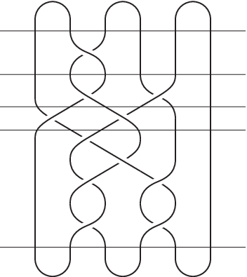
Next we study the distance of this $3$-bridge decomposition. Since the link $L$ is connected, the bridge decomposition cannot be separated into smaller ones. It follows that the distance is at least one. Consider the simple closed curve $c$ as in Figure 4. The curve $c$ is essential in $P\setminus L$ and disjoint from both $p(t_{+}^{1})$ and $p(t_{-}^{1})$. Recall that the boundary of a small neighborhood of $p(t_{+}^{1}),p(t_{-}^{1})$ in $P$ bounds an essential disk $D_{+}^{1}$ of $T_{+}$ and an essential disk $D_{-}^{1}$ of $T_{-}$, respectively. So there are an edge between $[\partial D_{+}^{1}],[c]$ and an edge between $[c],[\partial D_{-}^{1}]$ in the curve graph ${\mathcal{C}}(P\setminus L)$. By definition, the distance is at most two. It is true that there is no direct edge between $[\partial D_{+}^{1}]$ and $[\partial D_{-}^{1}]$. However, this is not enough to conclude that the distance is equal to two because there are infinitely many essential disks of $T_{+},T_{-}$ other than $D_{+}^{1},D_{-}^{1}$.

As shown in [2], [4], [8] and [9], sufficiently complicated Heegarrd diagram implies a large distance of the Heegaard splitting. We can expect that sufficiently complicated bridge diagram also implies a large distance of the bridge decomposition. A bridge diagram should be pretty complicated if it satisfies the well-mixed condition, which we define in the following.

Denote the arcs of each $\tau_{\varepsilon}$ by $t_{\varepsilon}^{1},t_{\varepsilon}^{2},\ldots,t_{\varepsilon}^{n}$. Let $l$ be a loop on $P$ containing $p(\tau_{-})$ such that $p(t_{-}^{1}),p(t_{-}^{2}),\ldots,p(t_{-}^{n})$ are located in $l$ in this order. We can assume that $p(\tau_{+})$ has been isotoped in $P\setminus L$ to have minimal intersection with $l$. For the bridge diagram of Figure 3, it is natural to choose $l$ to be the closure in $P\cong S^{2}$ of the horizontal line containing $p(t_{-}^{1})\cup p(t_{-}^{2})\cup p(t_{-}^{3})$. Let $H_{+},H_{-}\subset P$ be the hemi-spheres divided by $l$ and let $\delta_{i}$ ($1\leq i\leq n$) be the component of $l\setminus p(\tau_{-})$ which lies between $p(t_{-}^{i})$ and $p(t_{-}^{i+1})$. (Here the indices are considered modulo $n$.) Let ${\mathcal{A}}_{i,j,\varepsilon}$ be the set of components of $p(\tau_{+})\cap H_{\varepsilon}$ separating $\delta_{i}$ from $\delta_{j}$ in $H_{\varepsilon}$ for a distinct pair $i,j\in\{1,2,\ldots,n\}$ and $\varepsilon\in\{+,-\}$. For example, Figure 5 displays ${\mathcal{A}}_{1,2,+}$ for the above bridge diagram. Note that ${\mathcal{A}}_{i,j,\varepsilon}$ consists of parallel arcs in $H_{\varepsilon}$.

As in Figure 5, the bridge diagram in Figure 3 amply satisfies the $(1,2,+)$-well-mixed condition. One can also check the $(i,j,\varepsilon)$-well-mixed condition for all the other combinations $(i,j,\varepsilon)=(1,2,-),(2,3,+),(2,3,-),(3,1,+),(3,1,-)$. Hence the bridge diagram in Figure 3 satisfies the well-mixed condition.

Firstly, consider an essential disk $D_{-}$ of $T_{-}$. Assume that $D_{-}$ has been isotoped so that $|\partial D_{-}\cap l|$ is minimal. Here, $|\cdot|$ denotes the number of connected components of a topological space.

Secondly, consider an essential disk $D_{+}$ of $T_{+}$. Assume that $D_{+}$ has been isotoped so that $|\partial D_{+}\cap p(\tau_{+})|$ is minimal.

Assume that the distance of $(T_{+},T_{-};P)$ is less than two. There are disjoint essential disks $D_{+},D_{-}$ of $T_{+},T_{-}$, respectively. If $\partial D_{-}$ contains a subarc connecting $\delta_{i}$ and $\delta_{j}$ in $H_{\varepsilon}$, it intersects all the arcs of ${\mathcal{A}}_{i,j,\varepsilon}$. In particular, if two arcs of ${\mathcal{A}}_{i,j,\varepsilon}$ are adjacent in $H_{\varepsilon}$, a subarc of $\partial D_{-}$ connects them directly. The above observations and the well-mixed condition are almost enough to lead to a contradiction, but only the following should be checked:

Theorem 1 implies that the $3$-bridge decomposition in Figure 2 has distance at least two. Since we have shown that it is at most two, the distance is exactly two. We can work out in this way fairly many $n$-bridge decompositions, especially for $n=3$.

References

- [1] D. Bachman and S. Schleimer, Distance and bridge position, Pacific J. Math. 219 (2005), no. 2, 221–235.
- [2] J. Berge, A closed orientable -manifold with distinct distance three genus two Heegaard splittings, arXiv:math.GT/0912.1315.
- [3] J. S. Birman, Plat presentations for link groups, Collection of articles dedicated to Wilhelm Magnus. Comm. Pure Appl. Math. 26 (1973), 673–678.
- [4] A. Casson and C. Gordon, Manifolds with irreducible Heegaard splittings of arbitrary large genus, Unpublished.
- [5] R. Crowell and R. Fox, Introduction to knot theory, Graduate Texts in Mathematics, 57, Springer-Verlag, New York-Heidelberg.
- [6] K. Hartshorn, Heegaard splittings of Haken manifolds have bounded distance, Pacific J. Math. 204 (2002), no. 1, 61–75.
- [7] J. Hempel, 3-manifolds as viewed from the curve complex, Topology 40 (2001), no. 3, 631–657.
- [8] J. H. Lee, Rectangle condition for irreducibility of Heegaard splittings, arXiv:math.GT/0812.0225.
- [9] M. Lustig and Y. Moriah, High distance Heegaard splittings via fat train tracks, Topology Appl. 156 (2009), no. 6, 1118–1129.
- [10] H.A. Masur and Y.N. Minsky, Geometry of the complex of curves. I. Hyperbolicity, Invent. Math. 138 (1999), no. 1, 103–149.
- [11] H.A. Masur and Y.N. Minsky, Geometry of the complex of curves. II. Hierarchical structure, Geom. Funct. Anal. 10 (2000), no. 4, 902–974.
- [12] H. Masur and S. Schleimer, The geometry of the disk complex, arXiv:math.GT/1010.3174.
- [13] M. Scharlemann and M. Tomova, Alternate Heegaard genus bounds distance, Geom. Topol. 10 (2006), 593–617.
- [14] M. Tomova, Multiple bridge surfaces restrict knot distance, Algebr. Geom. Topol. 7 (2007), 957–1006.