Random Deployment of Data Collectors
for Serving Randomly-Located Sensors

Taesoo Kwon and John M. Cioffi ^†^†thanks: T. Kwon and J. M. Cioffi are with the Department of Electrical Engineering, Stanford University, Stanford CA, 94305, USA (e-mail: tskwon80@stanford.edu, cioffi@stanford.edu)

Abstract

Recently, wireless communication industries have begun to extend their services to machine-type communication devices as well as to user equipments. Such machine-type communication devices as meters and sensors need intermittent uplink resources to report measured or sensed data to their serving data collector. It is however hard to dedicate limited uplink resources to each of them. Thus, efficient service of a tremendous number of devices with low activities may consider simple random access as a solution. The data collectors receiving the measured data from many sensors simultaneously can successfully decode only signals with signal-to-interference-plus-noise-ratio (SINR) above a certain value. The main design issues for this environment become how many data collectors are needed, how much power sensor nodes transmit with, and how wireless channels affect the performance. This paper provides answers to those questions through a stochastic analysis based on a spatial point process and on simulations.

Index Terms:

M2M, stochastic geometry, spatial reuse, outage probability, network design, Poisson point process.

I Introduction

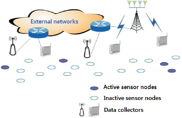
Wireless personal communication enables ubiquitous exchange of various data types such as voice, video, photos, and text among individuals. The emergence of new advanced systems such as the IEEE 802.11ac [1] and the 3GPP LTE-Advanced [2] are expected to achieve additional data rates. Of late, wireless communication industries have begun to discuss their scenarios serving machine-type communication devices such as meters/sensors as well as user equipments such as smart phones [3][4]. These machine-to-machine (M2M) communications have extensive applications, from monitoring environments to full electrical/mechanical automation (e.g. smart grid, smart city, Internet of things), which has been being considered as one of the most crucial technologies in future [5][6]. The sensor network can also be regarded as a kind of M2M, and there have been many studies in the form of ad-hoc networks [7][8]. This paper only considers the environment with specific data collectors directly communicating with sensors. This environment is suitable when sensor nodes support only simple single-hop communication functionalities and deployment of many data collectors is easy. This type of M2M communication is similar to cellular communication systems where the base stations serve user equipment within their coverage, but it has the unique characteristics [5][9]: there can be a huge number of devices (e.g. trillions) each of which has only a small amount of data and a low activity, and their functionalities have to be simple. These characteristics may require technologies differentiated from the conventional high data rate human-to-human (H2H) communications. For example, machine-type devices such as meters and sensors need uplink resources intermittently for reporting measured or sensed data to their serving data collector, but it is hard to dedicate limited uplink resources to each. Thus, simple random access can be considered as a solution for directly transmitting measured data or initially requesting uplink resources. The data collectors that receive many sensors’ measured data simultaneously can successfully decode only signals with signal-to-interference-plus-noise ratio (SINR) above a certain value. In order to keep a high success probability of many sensor nodes’ intermittent transmissions, the system may need a lot of data collectors, and conventional macro/micro base stations may not be appropriate for these roles. In other words, data collectors have to be easy to deploy and cost-effective. They support only simple functionalities and are interconnected with external networks through wired or wireless links. It can be considered that not only a new type of device for data collection is defined but also such devices as pico/femto base stations around sensor nodes play the role of data collectors. Fig. 1 shows a system architecture with data collectors and sensor nodes. In this environment, some questions are: How many data collectors are needed? How much transmit power sensors have to use for successful transmission? And, how the wireless channels affect the performance. This paper will provide answers to those questions through a stochastic analysis based on a spatial point process and on simulations.

The main factor of determining system performance is the interference from neighbor sensor nodes. This interference depends on the spatial distribution and sensor-node access methods. Because the spatial configurations of transmitting and receiving nodes can have enormous possibilities, it is impossible to consider each possibility. Stochastic geometry provides a useful mathematical tool to model network topology, and it also enables analysis of essential quantities such as interference distribution and outage [10][11][12]. This stochastic geometry has mainly been applied to pure ad hoc networks and their performance has been analyzed under the assumption of random transmitter location and receiver with fixed distances to its transmitter [10][13][14]. This paper considers the environment where both transmitters (sensor nodes) and receivers (data collectors) are randomly deployed and each transmitter are served by the data collector nearest to it. [15]-[19] have analyzed the distribution of signal-to-interference ratio (SIR) or SINR in random cellular networks where both transmitter and receiver are randomly located; [17] analyzed the distribution of SIR considering the path loss and shadowing, [18] derived a simple-form SINR distribution in case of Rayleigh fading and a path-loss exponent of four, and [19] expanded the analysis results in [18] into the results for a more general fading model including Nakagami- $m$ fading. But, they assumed that each base station always has the user equipment within its coverage and communicates with a user equipment that is scheduled exclusively within one cell and focused on transmitter-centric coverage (i.e. downlink). [20] modeled CDMA uplink interference power as a log-normal distribution using the moment-matching method. Also, [21] asymptotically analyzed uplink spectral efficiency in spatially distributed wireless networks, where the base stations have multiple antennas, by using infinite-random-matrix theory and stochastic geometry. The current system is similar to the uplink cellular systems, but this paper will only consider random access without any explicit scheduling for the simple functionalities of sensor nodes and data collectors.

The three contributions of this paper are: First, an analysis shows how the channel affects the SIR distribution for Nakagami- $m$ fading. A simple form on the SINR distribution is found for some special channel models. Second, an analysis describes how many data collectors per area are on average required to meet the outage probability for the given mean number of sensor nodes per area in case of Rayleigh fading. Third, this paper suggests a simple design method of the transmit power and the mean number of data collectors to meet the given outage probability.

The remainder of this paper is organized as follows: Section II presents the system model based on a homogeneous Poisson point process (PPP). Section III analyzes the SIR distribution for Nakagammi- $m$ fading channels and the SINR distribution for Rayleigh fading channels. Section IV derives the intensity of data collectors required to keep the outage probability below a certain value and suggests a design method of the transmit power. Section V discusses numerical results. Finally, Section VI concludes.

II System Model

A sensor node senses or measures environments and then transmits its data to the closest data collector. Sensor nodes do not always have data to transmit but send them only when their sensing data are generated. For example, machines such as meters and event sensors may transmit data intermittently rather than continuously, and it has to be successful with probability above a certain value. In order to model intermittent transmissions, the sensor node’s activity is defined as $\rho$ . This value of $\rho$ is between $0$ and $1$ , and this paper considers its small values. Meanwhile, data collectors that receive data from sensor nodes, are always ready to receive data from them.

This paper considers environments where both of sensor nodes and data collectors are randomly deployed. Sensor nodes are distributed according to a homogeneous PPP, $\Phi_{s}$ , and they transmit sensed data to their nearest data collectors through random access schemes. $\lambda_{s,total}$ denotes the intensity of sensor nodes that is the average number of them per area. In order to consider unplanned deployments of data collectors, the random locations of data collectors are modeled as a homogeneous PPP, $\Phi_{c}$ , with intensity $\lambda_{c}$ , like sensor nodes. Each sensor node transmits its data to a data collector closest to it, so a data collector builds a coverage based on Voronoi tessellation, as shown in Fig 2.

The standard power loss propagation model with the path loss exponent $\alpha(>2)$ and the Nakagami- $m$ fading model are considered. In the Nakagami- $m$ fading model [22], $m=1$ , $m=(K+1)^{2}/(2K+1)$ and $m=\infty$ model Rayleigh fading, Rician fading with parameter $K$ , and no fading, respectively. Also, it is assumed that all sensor nodes transmit with the same power $P$ . A typical data collector located on the origin receives the signal with $Pr^{-\alpha}G_{S}$ from a typical sensor node when the distance between them is $r$ and the fading channel gain is $G_{S}$ . By Slyvnyak’s theorem [23], interfering nodes except for a typical sensor node located on $X_{0}$ still constitute a homogeneous PPP with intensity $\lambda_{s,total}$ . Thus, the interference power of the link between a typical sensor node and a typical data collector can be expressed as $I_{r}=\sum_{X_{j}\in\Phi_{s}\backslash\{X_{0}\}}P\left|X_{j}\right|^{-\alpha}G_{I,j}$ where $X_{j}$ denotes the location of a interfering node and $G_{I,j}$ means the fading gain of a link between a typical data collector and a interfering sensor node $j$ . $\left\{G_{I,j}\right\}_{X_{j}\in\Phi_{s}\backslash\{X_{0}\}}$ are independently and identically distributed (i.i.d.) random variables. Here, it is assumed that a typical data collector does not perform any scheduling for sensor nodes within coverage served by itself, so they may interfere with each other even though they are served by a common data collector. Eventually, the link of a transmitter-receiver pair experiences interference from interfering nodes distributed according to a homogeneous PPP with effective intensity $\lambda_{s}=\lambda_{s,total}\cdot\rho$ . If a sensor transmits using one of $N$ resources that is chosen at random, $\lambda_{s}$ is $\lambda_{s,total}\cdot\rho/N$ . $\lambda_{s}$ decreases as $N$ increases and this means that $N$ is also a parameter for the system design. In this paper, $N=1$ is assumed.

When the interference is dealt with as noise and single antenna is equipped on both transmitters and receivers, the SINR is given by

\begin{array}[]{ll}\mathrm{SINR}&=\frac{P\left|X_{0}\right|^{-\alpha}G_{S}}{\sum_{X_{j}\in\Phi_{s}\backslash\{X_{0}\}}P\left|X_{j}\right|^{-\alpha}G_{I,j}+\sigma^{2}}\\ &=\frac{\left|X_{0}\right|^{-\alpha}G_{S}}{\sum_{X_{j}\in\Phi_{s}\backslash\{X_{0}\}}\left|X_{j}\right|^{-\alpha}G_{I,j}+\tilde{\sigma}^{2}}\end{array}

(1)

where $\sigma^{2}$ is the noise power and $\tilde{\sigma}^{2}$ is equal to $\frac{\sigma^{2}}{P}$ . In case of $\sigma^{2}\rightarrow 0$ , (1) means the SIR.

III SINR Distribution

This section analyzes the SINR distributions and derive simple-form SIR or SINR distribution for some specific channels. For more generalization of results, the fading gain distribution of (2) is first considered.

\Pr\left\{G_{S}>g\right\}=\sum_{n\in\mathcal{N}}\exp(-ng)\sum_{k\in\mathcal{K}}a_{nk}g^{k}

(2)

for some finite set $\mathcal{N}$ and a finite integer set $\mathcal{K}$ . This type of complementary cumulative distribution function (CCDF) includes a variety of fading-gain distributions such as exponential distribution, chi-square distribution and gamma distribution.

Lemma III.1

Let sensor nodes and data collectors distributed with homogeneous PPP’s with intensities $\lambda_{s}$ and $\lambda_{c}$ , respectively and each sensor node builds communication link with a data collectors closest to it. When the CCDF of the fading gain of a desired signal is given by (2) and the fading gain of the interfering signal is denoted as a random variable, $G_{I}$ , the CCDF of SINR is given by

\begin{array}[]{ll}\Pr\left\{{\rm SINR}>\beta\right\}\\ =2\pi\lambda_{c}\sum_{n\in\mathcal{N}}\sum_{k\in\mathcal{K}}a_{nk}\left(-\beta\right)^{k}\\ \int_{0}^{\infty}r^{k\alpha+1}\left.\frac{d^{k}\exp\left(-\lambda_{s}\xi(\zeta,\alpha)-\zeta\tilde{\sigma}^{2}\right)}{d\zeta^{k}}\right|_{\zeta=n\beta r^{\alpha}}\exp\left(-\lambda_{c}\pi r^{2}\right)dr\end{array}

(3)

where $\xi(\zeta,\alpha)=\pi\zeta^{\frac{2}{\alpha}}\Gamma\left(1-\frac{2}{\alpha}\right)\mathrm{E}\{G_{I}^{\frac{2}{\alpha}}\}$ , $\mathrm{E}\{x\}$ is the expectation of $x$ and $\Gamma(x)=\int_{0}^{\infty}t^{x-1}\exp(-t)dt$ denotes the gamma function. The derivative in (3) can be reexpressed as follow.

\begin{array}[]{ll}\frac{d^{k}\exp\left(-\lambda_{s}\xi(\zeta,\alpha)-\zeta\tilde{\sigma}^{2}\right)}{d\zeta^{k}}=\\ \exp\left(-\lambda_{s}\xi(\zeta,\alpha)-\zeta\tilde{\sigma}^{2}\right)\sum_{l=0}^{k}\frac{1}{l!}\sum_{j=0}^{l}(-1)^{l+j}\binom{l}{j}\\ \hskip 28.45274pt\left[\lambda_{s}\xi(\zeta,\alpha)+\zeta\tilde{\sigma}^{2}\right]^{j}\frac{\partial^{k}}{\partial\zeta^{k}}\left[\lambda_{s}\xi(\zeta,\alpha)+\zeta\tilde{\sigma}^{2}\right]^{l-j}\end{array}

(4)

Proof:

See Appendix A. ∎

The result of SINR distribution in Lemma III.1 requires cumbersome integrations and differentiations, but simple-form result can be obtained for specific channel models.

To begin with, an analysis considers Nakagami- $m$ fading channel. The received signal power experiencing Nakagami- $m$ fading channel can be modeled using Gamma distributions. Thus, assuming that desired signals experience Nakagami- $m_{s}$ fading while interfering signals experience Nakagami- $m_{i}$ fading, the CCDF of fading gains can be give by

\Pr\left\{G_{S}>g\right\}=\sum_{k=0}^{m_{s}-1}\frac{(m_{s}g)^{k}}{k!}\exp(-m_{s}g)

(5)

\Pr\left\{G_{I}>g\right\}=\sum_{k=0}^{m_{i}-1}\frac{(m_{i}g)^{k}}{k!}\exp(-m_{i}g)

(6)

(5) and (6) have the forms of (2), so the SINR distribution can be derived by using Lemma III.1. Generally, Lemma III.1 requires the calculation of a derivative in (4) and it is too complex to calculate it for any $m_{s}$ , $\alpha$ and $\tilde{\sigma}$ . Fortunately, it is possible to obtain a simple form for the CCDF of SINR under interference limited environments, i.e. $\sigma^{2}\rightarrow 0$ .

Proposition III.1

Let sensor nodes be randomly located with intensity $\lambda_{s}$ and served by the nearest data collectors randomly deployed with intensity intensity $\lambda_{c}$ . When their links experience Nakagami- $m$ fading given by (5) and (6), and $\tilde{\sigma}\rightarrow 0$ , the CCDF of SIR is given by

\begin{array}[]{ll}\Pr\left\{{\rm SIR}>\beta\right\}=\frac{\lambda_{c}}{\lambda_{c}+\lambda_{s}C(m_{i},\alpha)(m_{s}\beta)^{\frac{2}{\alpha}}}\cdot\\ \sum_{k=0}^{m_{s}-1}\frac{1}{k!}\sum_{l=0}^{k}(-1)^{l+k}\Delta_{k,l}\left[\frac{\lambda_{s}C(m_{i},\alpha)(m_{s}\beta)^{\frac{2}{\alpha}}}{\lambda_{c}+\lambda_{s}C(m_{i},\alpha)(m_{s}\beta)^{\frac{2}{\alpha}}}\right]^{l}\end{array}

(7)

where $C(m,\alpha)=\frac{m^{-\frac{2}{\alpha}}\Gamma\left(1-\frac{2}{\alpha}\right)\Gamma\left(m+\frac{2}{\alpha}\right)}{\Gamma\left(m\right)}$ and $\Delta_{k,l}=\sum_{j=0}^{l}(-1)^{j}\binom{l}{j}\prod_{i=0}^{k-1}\left[\frac{2}{\alpha}(l-j)-i\right]$ for $l\leq k$ . Here, $\Delta_{0,0}$ is defined as $1$ .

Proof:

See Appendix B. ∎

In Nakagami- $m$ fading model, $m=1$ means the Rayleigh fading model. Thus, it is also easy to obtain the CCDF of the SIR for Rayleigh fading model.

Corollary III.1

Let sensor nodes be randomly located with intensity $\lambda_{s}$ and served by the nearest data collector randomly deployed with intensity intensity $\lambda_{c}$ . When all links experience Rayleigh fading with unit mean, and $\tilde{\sigma}\rightarrow 0$ , the CCDF of SIR is given by

\begin{array}[]{ll}\Pr\left\{{\rm SIR}>\beta\right\}=\frac{\lambda_{c}}{\lambda_{c}+\lambda_{s}C(1,\alpha)\beta^{\frac{2}{\alpha}}}\end{array}

(8)

where $C(1,\alpha)=\Gamma\left(1-\frac{2}{\alpha}\right)\Gamma\left(1+\frac{2}{\alpha}\right)=\frac{2\pi}{\alpha\sin(2\pi/\alpha)}$ .

Proof:

By substituting $m_{s}=1$ and $m_{i}=1$ into the results in Proposition III.1, (8) is obtained. Also, $C(1,\alpha)$ can be calculated by using the property of the gamma function $\Gamma(1-z)\Gamma(z)=\frac{\pi}{\sin(\pi z)}$ . ∎

As discussed before, when the noise power cannot be neglected, it is hard to obtain a simple form of the SINR for general $m_{s}$ because it requires the derivative of (4). However, when a path loss exponent, $\alpha$ , is equal to $4$ and the fading channel is modeled as Rayleigh fading, the CCDF of SINR is simplified into a common integral form.

Proposition III.2

Let sensor nodes be randomly located with intensity $\lambda_{s}$ and served by the nearest data collector randomly deployed with intensity intensity $\lambda_{c}$ . when all links experience Rayleigh fading with unit mean and a path loss exponent $\alpha$ is $4$ , the CCDF of SINR is given by

\begin{array}[]{ll}\Pr\left\{{\rm SINR}>\beta\right\}\\ =\frac{\pi^{\frac{3}{2}}\lambda_{c}}{2\sqrt{\beta\tilde{\sigma}^{2}}}\exp\left(\frac{[\pi\lambda_{c}+K\beta^{\frac{1}{2}}\lambda_{s}]^{2}}{4\beta\tilde{\sigma}^{2}}\right){\rm erfc}\left(\frac{\pi\lambda_{c}+K\beta^{\frac{1}{2}}\lambda_{s}}{2\sqrt{\beta\tilde{\sigma}^{2}}}\right)\end{array}

(9)

where $K=\frac{\pi^{2}}{2}$ and ${\rm erfc}(x)=\frac{2}{\sqrt{\pi}}\int_{x}^{\infty}\exp\left(-t^{2}\right)dt$ is the complementary error function.

Proof:

The CCDF of fading gain for $m_{s}=1$ is the case of $\mathcal{N}=\left\{1\right\}$ , $\mathcal{K}=\left\{0\right\}$ and $a_{10}=1$ in (2). Thus, when $\alpha=4$

\begin{array}[]{ll}\Pr\left\{{\rm SINR}>\beta\right\}\\ =2\pi\lambda_{c}\int_{0}^{\infty}r\cdot\exp\left(-\pi r^{2}\left[\lambda_{s}\beta^{\frac{1}{2}}C(1,4)+\lambda_{c}\right]-\beta r^{4}\tilde{\sigma}^{2}\right)dr\end{array}

(10)

(10) follows from (3) and (23), and it can be evaluated by using the change of variables $r^{2}\rightarrow x$ and the integration formula, $\int_{0}^{\infty}\exp\left(-\left[ax+bx^{2}\right]\right)dx=\frac{1}{2\sqrt{b}}\exp\left(\frac{a^{2}}{4b}\right){\rm erfc}\left(\frac{a}{2\sqrt{b}}\right)$ for $a\geq 0$ and $b>0$ . Here, $K=\pi C(1,4)=\frac{\pi^{2}}{2}$ . ∎

Proposition III.2 is the result for $\alpha=4$ . When $\alpha$ is not $4$ , the CCDF of SINR can be expressed by generalized hypergeometric functions. But they are not simple, so this paper does not deal with them.

IV Intensity of Data Collectors

When sensor nodes are spatially distributed according to a homogeneous PPP with a certain intensity, it is important to decide how many data collectors should be deployed in order to keep the success probability of random accesses above a certain value. This section analyzes the requirement of the intensity of data collectors deployed at random, and the effect of channels on its required intensity, given the intensity of sensor nodes and a target outage probability. The outage probability, $\varepsilon$ , is defined as $\Pr\{{\rm SINR<\beta_{t}}\}$ where $\beta_{t}$ is the minimal SINR value required for the successful receptions.

The required intensity of data collectors for Rayleigh fading is presented in Corollary IV.1 and Proposition IV.1.

Corollary IV.1

Let sensor nodes randomly located with intensity $\lambda_{s}$ and served by the nearest data collectors. It is assumed that all links experience Rayleigh fading with unit mean and $\tilde{\sigma}\rightarrow 0$ . The necessary and sufficient condition of the intensity of data collectors randomly deployed, $\lambda_{c}$ , for keeping the outage probability below $\varepsilon_{t}$ , is

\begin{array}[]{ll}\lambda_{c}\geq\frac{1}{\varepsilon_{t}}(1-\varepsilon_{t})C(1,\alpha)\beta_{t}^{\frac{2}{\alpha}}\lambda_{s}\end{array}

(11)

where $C(1,\alpha)$ is defined in Corollary III.1.

Proof:

(11) can be directly derived from (8). ∎

Proposition IV.1

Let sensor nodes randomly located with intensity $\lambda_{s}$ and served by the nearest data collectors. It is assumed that all links experience Rayleigh fading with unit mean and $\alpha=4$ . The sufficient condition of the intensity of data collectors randomly deployed, $\lambda_{c}$ , for keeping the outage probability below $\varepsilon_{t}$ , is

\begin{array}[]{ll}\lambda_{c}\geq\frac{K\beta_{t}^{\frac{1}{2}}}{2\pi\varepsilon_{t}}\left[(1-2\varepsilon_{t})+\sqrt{1+8\varepsilon_{t}(1-\varepsilon_{t})\frac{\tilde{\sigma}^{2}}{(K\lambda_{s})^{2}}}\right]\lambda_{s}\end{array}

(12)

where $K=\frac{\pi^{2}}{2}$ .

Proof:

See Appendix C. ∎

The condition of $\lambda_{c}$ in (11) under interference-limited environments is necessary and sufficient while the condition in (12) under environments with non-neglectable noise is just sufficient. In fact, (12) has been derived from a lower bound of the complementary error function. But, for small values of $\tilde{\sigma}^{2}$ , (12) also gives a tight lower bound of $\lambda_{c}$ , and in particular, (12) is the same as (11) with $\alpha=4$ when $\tilde{\sigma}^{2}\rightarrow 0$ .

Here, given $\beta_{t}$ , $\varepsilon_{t}$ , $\sigma^{2}$ and $\lambda_{s}$ , the design method of the transmit power ( $P$ ) of sensor nodes and the intensity ( $\lambda_{c}$ ) of data collectors is suggested, for a path loss exponent of four. The relations among these variables are given by (9), but it is not easy to use (9) directly for the design of $P$ and $\lambda_{c}$ . On the contrary, the lower bound of the CCDF of SINR with a simpler form of (27) can give a simple design method for them. The lower bound of SINR CCDF in (27) is equivalent to the intensity condition of data collectors of (12) and the second term within a square root in (12) approximately models the effect of noise. Now, the transmit power and the intensity of data collectors can be separately designed. First, for neglecting the noise effect, the second term within the square root of (12) has to be much smaller that $1$ . The definition of $\tilde{\sigma}^{2}$ gives a condition of the transmit power.

\begin{array}[]{ll}8\varepsilon_{t}(1-\varepsilon_{t})\frac{\sigma^{2}/P}{(K\lambda_{s})^{2}}\stackrel{{\scriptstyle\mathrm{(a)}}}{{\leq}}\frac{8\sigma^{2}/P}{(\pi^{2}\lambda_{s})^{2}}\ll 1\end{array}

(13)

where (a) follows from the inequality of arithmetic and geometric means and the definition of $K$ . Thus, the transmit power can be set to

\begin{array}[]{ll}P=c\cdot\frac{8\sigma^{2}}{\pi^{4}\lambda_{s}^{2}}\end{array}

(14)

where $c$ is a constant much less than one and it is a design parameter. $c$ has to be set not only to neglect the noise power but also to keep transmit power as small as possible for sensor node’s power saving. Next, the intensity of data collectors can be designed according to (11) because the intensity condition (12) is almost equal to (11) if $P$ is set by (14). In this design, the transmit power is reciprocally proportional to $\lambda_{s}^{2}$ and this means that the longer the distance among sensor nodes is, the larger the required transmit power is, because of the noise effect, when the intensity of data collector is determined by (11). Even though this design method is very simple, but it gives a good design method for the random deployment of data collectors to serve randomly distributed wireless sensors. Its performances will be shown in Section V.

In interference-limited environments with Rayleigh fading channels, Corollary IV.1 shows the effect of the path loss exponents obviously. Because the function $\frac{x}{\sin x}$ is a increasing function of $0<x<\pi$ , it is obvious that the required density of data collectors decreases as the path loss exponent increases, when $\alpha>2$ and $\beta_{t}\geq 1$ for given $\varepsilon_{t}$ and $\lambda_{s}$ , from the definition of $C(1,\alpha)$ and (11).

On the contrary, it is not easy to express the required intensity of date collectors in case of the Nakagami- $m$ fading with general $m$ ’s, in a simple form. Here, the effect of wireless channels on system designs is analyzed by comparing the performances to those of Rayleigh fading, rather than deriving their requirements exactly, only when $\tilde{\sigma}^{2}\rightarrow 0$ . When deploying data collectors with intensity $\lambda_{c,o}$ for randomly distributed sensor nodes with intensity $\lambda_{s}$ , let $\varepsilon^{(o)}$ and $\varepsilon^{(m)}$ denote the outage probabilities for the Rayleigh fading model and the another examined-fading model for the required SIR $\beta_{t}$ , respectively. First, in case of reference channel model assuming the Rayleigh fading, the $\lambda_{c,o}$ and $\varepsilon^{(o)}$ have the following relation from (9).

\begin{array}[]{ll}\lambda_{c,o}=\frac{1}{\varepsilon^{(o)}}(1-\varepsilon^{(o)})C(1,\alpha)\beta_{t}^{\frac{2}{\alpha}}\lambda_{s}\end{array}

(15)

On the other hand, in case of the examined-fading channel, $\tilde{\lambda}_{c,m}$ is defined as

\begin{array}[]{ll}\tilde{\lambda}_{c,m}=\frac{1}{\varepsilon^{(m)}}(1-\varepsilon^{(m)})C(1,\alpha)\beta_{t}^{\frac{2}{\alpha}}\lambda_{s}\end{array}

(16)

where $\varepsilon^{(m)}$ is derived from (7). In other words, (16) means that the deployment of data collectors with $\lambda_{c,o}$ in the Nakagami- $m$ fading channel is equal to the deployment of data collectors with $\tilde{\lambda}_{c,m}$ in the Rayleigh fading channel in term of outage probability. Hence, $\tilde{\lambda}_{c,m}/\lambda_{c,o}$ quantifies the effect of wireless fading channels on the system design and is simplified from (15) and (16), as follows.

\begin{array}[]{ll}\frac{\tilde{\lambda}_{c,m}}{\lambda_{c,o}}=\frac{\varepsilon^{(o)}(1-\varepsilon^{(m)})}{\varepsilon^{(m)}(1-\varepsilon^{(o)})}=\frac{1/\varepsilon^{(m)}-1}{1/\varepsilon^{(o)}-1}\end{array}

(17)

V Numerical Results and Discussion

This section evaluates and discusses the performance of systems with data collectors randomly deployed to serve randomly distributed wireless sensors, based on results of Section III and Section IV. It is assumed that the total intensity of sensor nodes ( $\lambda_{s,total}$ ) spatially distributed according to a homogeneous PPP is $10^{-2}{\rm m}^{-2}$ . Also, $\rho$ is set to $10^{-4}$ and it means that the sensor nodes awake on average every $1000$ sec (about 17 minutes), when they transmit data to data collectors during $100$ msec on each awake mode. Also, the minimal SINR value ( $\beta_{t}$ ) required for the successful reception of $0$ dB is considered.

Fig. 3 shows the CDF of SINR according to $P$ and $\frac{\lambda_{c}}{\lambda_{s}}$ . This can be interpreted as the outage probability for $\beta_{t}$ which is a value on x-axis. $P/\sigma^{2}$ ’s (or $1/\tilde{\sigma}^{2}$ ) of $100$ dB and $120$ dB are assumed. These values mean that the transmit powers of sensor nodes are $-10$ dBm ( $0.1$ mW) and $10$ dBm ( $10$ mW), when the power spectral density of the noise is $-170$ dBm/Hz and the bandwidth is $1$ MHz. Fig. 3 indicates that analysis results in (8) and (9) definitely coincide with the simulation results. When $P/\sigma^{2}$ is $100$ dB, the $\frac{\lambda_{c}}{\lambda_{s}}$ ’s of $10$ and $20$ result in the outage probabilities of $0.23$ and $0.1$ , respectively. As $P/\sigma^{2}$ increases, outage probability decreases. In other words, larger intensity of data collectors and higher transmit power lead to less outage probability. Fig. 4 and Fig. 5 explain these effects more quantitatively. In Fig. 4, the outage probability decreases as the intensity of data collectors increases, and their required intensity can be obtained for a given outage probability. Also its lower bound by (12) is shown. The lower bound of $\lambda_{c}$ in (12) is tighter when the effect of noise is reduced. The effect of noise on outage probability decreases as $\frac{\lambda_{c}}{\lambda_{s}}$ increases. This is because the increase of $\frac{\lambda_{c}}{\lambda_{s}}$ leads to the increase of received SNR because of the decrease in distances between data collectors and sensor nodes. Fig. 5 shows how the transmit power of sensor nodes affect the outage probability. The results of Fig. 5 were evaluated by changing the intensity of sensor nodes for given relative intensities of data collectors. In other words, it shows the effect of noise by changing the geometric size of networks. The larger geometric size, i.e. larger distances between sensor nodes and data collectors, leads to the bigger effects of noise on the system performance. These results also verify that the design of the transmit power not only reduces the noise effect but also keeps the transmit power as small as possible. Also, under the environments of Fig. 3, the design by (14) with $c=0.1$ provides the transmit power of $9$ dBm (i.e. $P/\sigma^{2}=119$ dB), and it is observed that $P/\sigma^{2}=120$ dB approaches the performance of $P/\sigma^{2}\rightarrow\infty$ in Fig. 3. These results confirm that (14) is a very efficient design method. The path loss exponent is another crucial factor to have an effect on system performances. As Fig. 6 indicates, they result in very different performance for the same transmit power. At $P/\sigma^{2}=100$ dB, the noise can be neglected in case of a pathloss exponent $3$ while it causes severe performance degradation in case of a pathloss exponent $5$ . By contrast, when the noise effect can be neglected, larger $\alpha$ ’s result in less outage probability for given $\beta_{t}$ and $\lambda_{s}$ . In fact, for given $\varepsilon_{t}$ and $\lambda_{s}$ , the required $\lambda_{c}$ for a pathloss exponent of $\alpha^{\prime}$ increases by the factor of $\frac{C(1,\alpha^{\prime})}{C(1,\alpha)}\beta_{t}^{(\frac{2}{\alpha^{\prime}}-\frac{2}{\alpha})}$ , compared to a pathloss exponent of $\alpha$ when $P/\sigma^{2}\rightarrow 0$ , where $C(1,\alpha)$ is defined in Corollary IV.1. For example, when $\beta_{t}=0~\rm{dB}$ , the path loss exponents of $3$ and $5$ requires $1.54$ and $0.84$ times of the intensity of data collectors for the path loss exponent of $4$ .

Fig. 7 - Fig. 9 examine the performance for Nakagami- $m$ fading channels. Fig. 7 explains how the line-of-sight factors of fading channels contribute to the SINR distribution. The increase in $m$ results in the decrease in outage probability. But, $m$ more than two does not have an big effect on the performance, compared to $m$ equal to two. Fig. 7 also indicates that analysis results exactly coincide with simulation results when considering that the performance of $P/\sigma^{2}=120$ dB is as good as that of $P/\sigma^{2}\rightarrow\infty$ . Fig. 8 shows the effect of channels on outage probability under the interference-limited environments. The outage probability decreases as $m$ and the pathloss exponent increase. It means that the Rician fading and AWGN environments need less intensity of data collectors than the Rayleigh fading environments for the same path loss exponent. Moreover, from this figure, the intensity of data collectors required to meet a certain outage probability can be obtained. Fig. 9 examines the relative effect of other fading channels compared to the Rayleigh fading channel in term of the intensity of data collectors, which is defined in (17). it shows that $m$ and $\alpha$ has a big effect on the system design such as the deployment of data collectors.

So far, this paper analyzed and discussed the effect of the wireless channels, the transmit power and the intensity of data collectors on system performances when data collectors are randomly deployed to successfully collect the data from randomly-located sensor nodes. As the number of wireless nodes increases enormously in future, it is more and more difficult to design the system. For reducing these difficulties, efficient system design methods is required to deal with a huge number of wireless nodes, so the rigorous understanding about the spatial distribution and effect of interference will be basics for them. Even though this paper has considered only simple random access, these results will be able to be used as basic models for developing more sophisticated spatial resource management methods.

VI Conclusions

This paper has considered the environment where receivers (data collectors) as well as transmitters (sensor nodes) are randomly deployed and each transmitter is served by the receiver nearest to it. In network topology modeled by homogeneous Poisson point processes, analysis and simulation results showed the SINR distribution, and a simple design method of transmit power was suggested. Under interference-limited environments, the larger the path loss exponent and the portion of line-of-site factors were, the less the outage probability was. On the contrary, under non-neglectable noise environments, the large path loss exponent caused severe performance degradation. Moreover, the intensity of data collectors required to keep the outage probability above a certain value was derived, and it depends on required outage probability, an intensity of sensor nodes, a fading channel model, a path loss exponent and noise power. This required intensity helps to design such parameters as the amount of wireless resources and the access probability for medium access control. Random access scheme is very simple and does not cause control-overhead problems even under environments with a huge number of sensor nodes, but its required intensity of data collectors is never small. Thus, it is needed to find more sophisticated spatial resource management schemes and the result of this paper may be used as a basic model for them.

Appendix A Proof of Lemma III.1

This proof is similar to proof of theorem 1 in [19] that has considered the transmitter-centric coverage (or downlink) and only the transmitter intensity. Here, an analysis focuses on the receiver-centric coverage by data collectors (or uplink) and allows that multiple transmitters within the service area of a common data collector simultaneously transmit. For those differences and the completeness, this paper provides the full derivation of the CCDF of SINR.

The probability that there is a data collector at a distance of $r$ from a typical sensor node is $2\pi\lambda_{c}dr$ . For this data collector to be a serving data collector of a typical sensor node, all other data collectors must be farther than $r$ from a typical sensor node, and its probability is $\exp(-\lambda_{c}\pi r^{2})$ . Thus, the probability density function of the distance between a typical sensor node and its serving data collector, $f_{r}(r)$ , is equal to $2\pi\lambda_{c}r\cdot\exp(-\lambda_{c}\pi r^{2})$ .

The CCDF of SINR is

\begin{array}[]{ll}\Pr\{{\rm SINR}>\beta\}\\ =\int_{0}^{\infty}\Pr\left\{\frac{r^{-\alpha}G_{S}}{I_{r}+\tilde{\sigma}^{2}}>\beta\right\}f_{r}(r)dr\\ =2\pi\lambda_{c}\int_{0}^{\infty}\Pr\left\{G_{S}>\beta r^{\alpha}(I_{r}+\tilde{\sigma}^{2})\right\}r\exp(-\lambda_{c}\pi r^{2})dr\end{array}

(18)

where $I_{r}=\sum_{X_{j}\in\Phi_{s}\backslash\{X_{0}\}}\left|X_{j}\right|^{-\alpha}G_{I,j}$ . From (2),

\begin{array}[]{ll}\Pr\left\{G_{S}>\beta r^{\alpha}(I_{r}+\tilde{\sigma}^{2})\right\}\\ =\mathrm{E}_{I_{r}}\left\{\sum_{n\in\mathcal{N}}\exp(-n\beta r^{\alpha}[I_{r}+\tilde{\sigma}^{2}])\cdot\right.\\ \hskip 71.13188pt\left.\sum_{k\in\mathcal{K}}a_{nk}(\beta r^{\alpha}[I_{r}+\tilde{\sigma}^{2}])^{k}\right\}\\ =\sum_{n\in\mathcal{N}}\sum_{k\in\mathcal{K}}a_{nk}(\beta r^{\alpha})^{k}\cdot\\ \hskip 71.13188pt\mathrm{E}_{I_{r}}\left\{(I_{r}+\tilde{\sigma}^{2})^{k}\exp(-n\beta r^{\alpha}[I_{r}+\tilde{\sigma}^{2}])\right\}\\ \stackrel{{\scriptstyle\mathrm{(a)}}}{{=}}\sum_{n\in\mathcal{N}}\sum_{k\in\mathcal{K}}a_{nk}(-\beta r^{\alpha})^{k}\left.\frac{d^{k}\mathrm{E}\{\exp\left(-\zeta(I_{r}+\tilde{\sigma}^{2})\right)\}}{d\zeta^{k}}\right|_{\zeta=n\beta r^{\alpha}}\\ \stackrel{{\scriptstyle\mathrm{(b)}}}{{=}}\sum_{n\in\mathcal{N}}\sum_{k\in\mathcal{K}}a_{nk}(-\beta r^{\alpha})^{k}\left.\frac{d^{k}\mathcal{L}_{I_{r}}(\zeta)\exp(-\zeta\tilde{\sigma}^{2})}{d\zeta^{k}}\right|_{\zeta=n\beta r^{\alpha}}\end{array}

(19)

where (a) and (b) follow from the definition of Laplace transform, $\mathcal{L}_{X}(\zeta)=\mathrm{E}_{X}\{\exp(-\zeta X)\}$ , its property, $\mathcal{L}_{t^{k}X(t)}(\zeta)=(-1)^{k}\frac{d^{k}\mathcal{L}_{X}(\zeta)}{d\zeta^{k}}$ , and the independence of $I_{r}$ and $\tilde{\sigma}^{2}$ . The Laplace transform of $I_{r}$ is

\begin{array}[]{ll}\mathcal{L}_{I_{r}}(\zeta)&=\mathrm{E}_{I_{r}}\{\exp(-\zeta I_{r})\}\\ &=\mathrm{E}_{\Phi_{s},G_{I}}\{\exp(-\zeta\sum_{X_{j}\in\Phi_{s}\backslash\{X_{0}\}}\left|X_{j}\right|^{-\alpha}G_{I,j})\}\\ &=\mathrm{E}_{\Phi_{s}}\{\prod_{X_{j}\in\Phi_{s}\backslash\{X_{0}\}}\mathrm{E}_{G_{I,j}}\{\exp(-\zeta G_{I,j}\left|X_{j}\right|^{-\alpha})\}\}\\ &\stackrel{{\scriptstyle\mathrm{(c)}}}{{=}}\exp\left(-2\pi\lambda_{s}\int_{0}^{\infty}[1-\mathrm{E}_{G_{I}}\{\exp(-\zeta G_{I}v^{-\alpha})\}]vdv\right)\\ &\stackrel{{\scriptstyle\mathrm{(d)}}}{{=}}\exp\left(-2\pi\lambda_{s}\cdot\right.\\ &\hskip 36.98866pt\left.\int_{0}^{\infty}\left(\int_{0}^{\infty}[1-\exp(-\zeta v^{-\alpha}g]vdv\right)f_{G_{I}}(g)dg\right)\\ &\stackrel{{\scriptstyle\mathrm{(e)}}}{{=}}\exp\left(-\frac{2\pi\lambda_{s}\zeta^{\frac{2}{\alpha}}}{\alpha}\Gamma\left(-\frac{2}{\alpha}\right)\int_{0}^{\infty}g^{\frac{2}{\alpha}}f_{G_{I}}(g)dg\right)\\ &\stackrel{{\scriptstyle\mathrm{(f)}}}{{=}}\exp\left(-\lambda_{s}\xi(\zeta,\alpha)\right)\end{array}

(20)

where (c) follows from the probability generating functional (PGFL) of the PPP [23]; (d) uses the probability density function $f_{G_{I}}(g)$ of a random variable $G_{I}$ ; (e) follows from the change of variable $v^{-\alpha}\rightarrow x$ and the definition of the Gamma function; (f) follows from the property of Gamma function $x\Gamma(x)=\Gamma(1+x)$ and the definition of $\xi(\zeta,\alpha)$ .

By substituting (19) and (20) into (18), (3) is derived.

Also, (4) is obtained from the following equation which can be derived by the derivative of the exponential function and the chain rules:

\begin{array}[]{ll}\frac{\partial^{k}}{\partial z^{k}}\exp\left(f(z)\right)=\\ \exp\left(f(z)\right)\sum_{l=0}^{k}\frac{1}{l!}\sum_{j=0}^{l}(-1)^{j}\binom{l}{j}f(z)^{j}\frac{\partial^{k}f(z)^{l-j}}{\partial z^{k}}\end{array}

(21)

where $\binom{l}{j}$ denotes $\frac{l!}{j!(l-j)!}$ .

Appendix B Proof of Proposition III.1

The fading gain of Nakagami- $m$ fading channel given in (5) can be reexpressed as

\Pr\left\{G_{S}>g\right\}=\sum_{n=m_{s}}^{m_{s}}\exp(-ng)\sum_{k=0}^{m_{s}-1}\frac{n^{k}}{k!}g^{k}

(22)

So, the Nakagami- $m$ fading is the case of $\mathcal{N}=\left\{m_{s}\right\}$ , $\mathcal{K}=\left\{0,\cdots,m_{s}-1\right\}$ and $a_{nk}=\frac{n^{k}}{k!}$ . Thus,

\begin{array}[]{ll}\xi\left(\zeta,\alpha\right)&=\pi\zeta^{\frac{2}{\alpha}}\Gamma\left(1-\frac{2}{\alpha}\right)\int_{0}^{\infty}g^{\frac{2}{\alpha}}\cdot\frac{g^{m_{i}-1}\exp(-m_{i}g)}{m_{i}^{-m_{i}}\Gamma(m_{i})}dg\\ &=\pi\zeta^{\frac{2}{\alpha}}C(m_{i},\alpha)\end{array}

(23)

where $C(m,\alpha)$ is defined as $\frac{m^{-\frac{2}{\alpha}}\Gamma\left(1-\frac{2}{\alpha}\right)\Gamma\left(m+\frac{2}{\alpha}\right)}{\Gamma\left(m\right)}$ .

When $\tilde{\sigma}^{2}\rightarrow 0$ , the derivative (4) is calculated into

\begin{array}[]{ll}\frac{d^{k}\exp\left(-\lambda_{s}\xi(\zeta,\alpha)\right)}{d\zeta^{k}}\\ =\exp\left(-\lambda_{s}\pi\zeta^{\frac{2}{\alpha}}C(m_{i},\alpha)\right)\sum_{l=0}^{k}\frac{1}{l!}\sum_{j=0}^{l}(-1)^{l+j}\binom{l}{j}\\ \hskip 28.45274pt\left[\lambda_{s}\pi\zeta^{\frac{2}{\alpha}}C(m_{i},\alpha)\right]^{j}\frac{\partial^{k}}{\partial\zeta^{k}}\left[\lambda_{s}\pi\zeta^{\frac{2}{\alpha}}C(m_{i},\alpha)\right]^{l-j}\\ =\exp\left(-\lambda_{s}\pi\zeta^{\frac{2}{\alpha}}C(m_{i},\alpha)\right)\sum_{l=0}^{k}\frac{1}{l!}\sum_{j=0}^{l}(-1)^{l+j}\binom{l}{j}\\ \hskip 28.45274pt[-\lambda_{s}\pi C(m_{i},\alpha)]^{l}\left[\prod_{i=0}^{k-1}\left(\frac{2}{\alpha}(l-j)-i\right)\right]\zeta^{\frac{2}{\alpha}l-k}\end{array}

(24)

From (22) and (24), (3) is

\begin{array}[]{ll}\Pr\left\{{\rm SIR}>\beta\right\}\\ \stackrel{{\scriptstyle\mathrm{(a)}}}{{=}}2\pi\lambda_{c}\sum_{k=0}^{m_{s}-1}\frac{m_{s}^{k}}{k!}(-\beta)^{k}\\ \hskip 28.45274pt\int_{0}^{\infty}(m_{s}\beta)^{-k}\sum_{l=0}^{k}\frac{(-1)^{l}}{l!}\left[\lambda_{s}\pi C(m_{i},\alpha)(m_{s}\beta)^{\frac{2}{\alpha}}r^{2}\right]^{l}\cdot\\ \hskip 28.45274pt\Delta_{k,l}\cdot\exp\left(-[\lambda_{s}\pi C(m_{i},\alpha)(m_{s}\beta)^{\frac{2}{\alpha}}+\lambda_{c}\pi]r^{2}\right)rdr\\ \stackrel{{\scriptstyle\mathrm{(b)}}}{{=}}2\pi\lambda_{c}\sum_{k=0}^{m_{s}-1}\frac{(-1)^{k}}{k!}\\ \hskip 28.45274pt\sum_{l=0}^{k}\frac{(-1)^{l}}{l!}\left[\lambda_{s}\pi C(m_{i},\alpha)(m_{s}\beta)^{\frac{2}{\alpha}}\right]^{l}\Delta_{k,l}\\ \hskip 28.45274pt\int_{0}^{\infty}\exp\left(-[\lambda_{s}\pi C(m_{i},\alpha)(m_{s}\beta)^{\frac{2}{\alpha}}+\lambda_{c}\pi]r^{2}\right)r^{2l+1}dr\\ \stackrel{{\scriptstyle\mathrm{(c)}}}{{=}}2\pi\lambda_{c}\sum_{k=0}^{m_{s}-1}\frac{(-1)^{k}}{k!}\\ \hskip 28.45274pt\sum_{l=0}^{k}\frac{(-1)^{l}}{l!}\left[\lambda_{s}\pi C(m_{i},\alpha)(m_{s}\beta)^{\frac{2}{\alpha}}\right]^{l}\Delta_{k,l}\\ \hskip 28.45274pt\left(\frac{1}{2}\left[\lambda_{s}\pi C(m_{i},\alpha)(m_{s}\beta)^{\frac{2}{\alpha}}+\lambda_{c}\pi\right]^{-l-1}\Gamma(l+1)\right)\\ \stackrel{{\scriptstyle\mathrm{(d)}}}{{=}}\frac{\lambda_{c}}{\lambda_{c}+\lambda_{s}C(m_{i},\alpha)(m_{s}\beta)^{\frac{2}{\alpha}}}\sum_{k=0}^{m_{s}-1}\frac{1}{k!}\cdot\\ \hskip 28.45274pt\sum_{l=0}^{k}(-1)^{k+l}\Delta_{k,l}\left[\frac{\lambda_{s}C(m_{i},\alpha)(m_{s}\beta)^{\frac{2}{\alpha}}}{\lambda_{c}+\lambda_{s}C(m_{i},\alpha)(m_{s}\beta)^{\frac{2}{\alpha}}}\right]^{l}\end{array}

(25)

where (a) follows from the definition of $\Delta_{k,l}$ in Proposition III.1, (b) follows from the interchange of a summation and an integration, (c) follows from the calculation of the integral part by the definition of the Gamma function, and (d) follows from the property of the Gamma function $\Gamma(l+1)=l!$ for a nonnegative integer $l$ .

Appendix C Proof of Proposition IV.1

Let $\tau=\frac{\pi\lambda_{c}+K\beta_{t}^{\frac{1}{2}}\lambda_{s}}{2\sqrt{\beta_{t}\tilde{\sigma}^{2}}}$ and $\kappa=\pi^{\frac{3}{2}}\frac{\lambda_{c}}{2\sqrt{\beta_{t}\tilde{\sigma^{2}}}}$ . (9) can be expressed as

\begin{array}[]{ll}\Pr\left\{{\rm SINR}>\beta\right\}=\exp(\tau^{2}){\rm erfc}(\tau)\kappa\\ \stackrel{{\scriptstyle\rm(a)}}{{>}}\exp(\tau^{2})\cdot\frac{2}{\sqrt{\pi}}\frac{\tau}{1+2\tau^{2}}\exp(-\tau^{2})\cdot\kappa\\ =\frac{2}{\sqrt{\pi}}\frac{\tau}{1+2\tau^{2}}\cdot\kappa\end{array}

(26)

where (a) follows from the lower bound of the complementary error function. From (9) and (26),

\begin{array}[]{ll}\Pr\left\{{\rm SINR}>\beta\right\}&\stackrel{{\scriptstyle\rm(b)}}{{>}}\pi\lambda_{c}\cdot\frac{\pi\lambda_{c}+K\beta_{t}^{\frac{1}{2}}\lambda_{s}}{2\beta_{t}\tilde{\sigma}^{2}+(\pi\lambda_{c}+K\beta_{t}^{\frac{1}{2}}\lambda_{s})^{2}}\\ &\geq 1-\varepsilon_{t}\end{array}

(27)

where (b) follows from the definition of $\tau$ and $\kappa$ . (27) is rewritten into

\begin{array}[]{ll}\varepsilon_{t}\pi^{2}\lambda_{c}^{2}-[(1-2\epsilon_{t})\pi K\beta_{t}^{\frac{1}{2}}\lambda_{s}]\lambda_{c}\\ \hskip 56.9055pt-(1-\varepsilon_{t})(K^{2}\beta_{t}\lambda_{s}^{2}+2\beta_{t}\tilde{\sigma}^{2})\geq 0\end{array}

(28)

which is a quadratic inequality with the form of $a\lambda_{c}^{2}+b\lambda_{c}+c\geq 0$ where $a>0$ and $c<0$ for $0<\varepsilon_{t}<1$ . Thus, (28) gives a positive lower bound of $\lambda_{c}$ . By solving the inequality (28) for a variable $\lambda_{c}>0$ , (12) is derived.

References

[1] IEEE ${\rm 802.11^{TM}}$ Wireless Local Area Networks, http://www.ieee802.org/11
[2] The 3rd Generation Partenership Project, http://www.3gpp.org
[3] 3GPP TS 22.368 v11.0.0, ”Service requirements for machine-type communications,” Dec. 2010
[4] 3GPP TR 23.888 v.1.0.0, ”System improvement for machine-type communications,” Sep. 2010
[5] S.-Y. Lien, K.-C. Chen, and Y. Lin, ”Toward ubiquitous massive accesses in 3GPP machine-to-machine communications,” IEEE Communications Magazine, vol. 49, no 4, pp. 66-74, Apr. 2011
[6] G. Wu, S. Talwar, K. Johnsson, Na. Himayat, and K. D. Johnson, ”M2M: from mobile to embedded internet,” IEEE Communications Magazine, vol. 49, no 4, pp. 36-43, Apr. 2011
[7] L. F. Akyildiz et al., ”A survey on sensor networks,” IEEE Communications Magazine, vol. 40, no. 8, pp. 102-114, Aug. 2002
[8] R. V. Kulkarni, A. Forster, and G. K. Venayagamoorthy, ”Computational intelligence in wireless sensor networks: a survey,” IEEE Communications Surveys & Tutorials, vol. 13, no. 1, pp. 68-96, Feb. 2011
[9] ETSI MCC, ”R2-101881: Report of 3GPP TSG RAN WG2 meeting 68bis,” 3GPP TSG RAN WG2 Meeting, 68bis, Feb. 2010
[10] M. Haenggi, J. G. Andrews, F. Baccelli, O. Dousse, and M. Franceschetti, ”Stochastic geometry and random graphs for the analysis and design of wireless networks,” IEEE Journal on Selected Area in Communications, vol. 27, no. 7, pp. 1029-1046, Sep. 2009
[11] F. Baccelli and B. Blaszczyszyn, Stochastic Geometry and Wireless Networks, NOW: Foundations and Trends in Networking, 2010
[12] J. G. Andrews, R. K. Ganti, M. Haenggi, N. Jindal, and S. Weber, ”A primer on spatial modeling and analysis in wireless networks,” IEEE Communications Magazine, vol. 48, no. 11, pp. 156-163, Nov. 2010.
[13] A. M. Hunter, J. G. Andrews, and S. P. Weber, ”Transmission capacity of ad hoc networks with spatial diversity”, IEEE Transactions on Wireless Communications, vol. 7, no. 12, pp. 5058-5071, Dec. 2008
[14] F. Baccelli, B. Blaszczyszyn, and P. Muhlethaler, ”Stochastic analysis of spatial and opportunistic aloha,” IEEE Journal of Selected Areas in Communications, vol 27. no. 7, pp. 1105-1119, Sep. 2009
[15] F. Baccelli, M. Klein, M. Lebourges, and S. Zuyev, ”Stochastic geometry and architecture of communication networks,” J. Telecommunication Systems, vol. 7, no. 1, pp. 209-227, Sep. 1995
[16] C. C. Chan and S. V. Hanly, ”Calculating the outage probability in a CDMA network with spatial Poisson traffic,” IEEE Transactions on Vehicular Technology, vol. 50, no. 1, pp. 183-204, Jan. 2001
[17] P. Madhusudhanan, J. G. Restrepoy, Y. Liu, and T. X. Brown, ”Carrier to interference ratio analysis for the shotgun cellular system,” in Proc. IEEE Globecom 2009, Nov. 2009
[18] J. G. Andrews, F. Baccelli, and R. K. Ganti, ”A tractable approach to coverage and rate in cellular networks”, submitted to IEEE Transactions on Communications, Sep. 2010
[19] R. K. Ganti, F. Baccelli, and J. G. Andrews ”A new way of computing rate in cellular networks,” in Proc. ICC 2011, Jun. 2011
[20] N. B. Mehta, S. Singh, and A. F. Molisch, ”An accurate model for interference from spatially distributed shadowed users in CDMA uplinks,” in Proc. IEEE Globecom 2009, Nov. 2009
[21] S. Govindasamy and D. H. Staelin, ”Asymptotic spectral efficiency of the uplink in spatially distributed wireless networks with multi-antenna base stations,” arXiv:1102.1232v1, Feb. 2011
[22] M. Nakagami, ”The $m$ -distribution- A General Formula of Intensity Distribution of Rapid Fading,” in Statistical Methods in Radio Wave Propagation (W. G. Hoffman, ed.), pp. 3-36, Pergamon Press, Oxford, England, 1960
[23] D. Stoyan, W. Kendall, and J. Mecke, Stochastic Geometry and Its Applications, 2nd Edition, John Wiley and Sons, 1996