Tunneling Time of Bose-Einstein Condensates on Real Time Stochastic Approach
Abstract
We study tunneling processes of Bose-Einstein condensate (BEC) on the real time stochastic approach and reveal some properties of their tunneling time. An important result is that the tunneling time decreases as the repulsive interatomic interaction becomes stronger. Furthermore, the tunneling time in a strong interaction region is not much affected by the potential height and is represented by an almost constant function. We also obtain the other related times such as the hesitating and interaction ones and investigate their dependence on the interaction strength. Finally, we calculate the mean arrival time of BEC wave packet and show the large displacement of its peak position.
pacs
03.75.Lm,42.25.Bs,03.65.Xp,03.65.SqI Introduction
The Bose-Einstein condensates (BECs) of trapped atoms, first realized in 1995 [1, 2, 3], are ideal systems for studying macroscopic quantum phenomena. This is because the systems are dilute, weakly interacting ones and we can easily control the configuration of the trap and even the strength of interatomic interaction. The BEC is described by a macroscopic wavefunction with nonlinear effects due to interatomic interactions and show the macroscopic tunneling phenomena such as Josephson oscillations. Many studies on BEC tunneling through various kinds of potentials [4, 5, 6] have already been done. We expect that the BECs give us new insights for nonlinear dynamics and macroscopic tunneling phenomena.
The problem of tunneling time for quantum particle is controversial, mainly because the time is not represented by an operator but is a parameter in quantum mechanics. It has been investigated for decades and many definitions of the tunneling time have been proposed [7, 8, 9, 10, 11, 12, 13, 14, 15, 16, 17, 18]. For example, the phase time [7] is expressed by an energy derivative of phase shift of transmitted wave from a potential barrier. The Larmor time [8, 9, 10] is obtained from the Larmor precession angle caused by a magnetic field in the potential barrier region. The Büttiker-Landauer time [11, 12, 13] is defined from transmission coefficient through a barrier with a small oscillation of height. There are methods based on the concept of “particle path” such as Bohmian mechanics [14, 15], Feynman path integral [16, 17], Nelson’s stochastic approach [18, 19, 20, 21] and so on. The cold atomic gas systems are promising to investigate the tunneling time of quantum particle, since their dynamical behaviors can be observed in detail and one can even control several parameters such as the configuration of trap, the strength of interatomic interaction and the internal degree of freedom such as spin.
In this paper, we focus on the tunneling time associated with BEC wave function and its dependence on the interaction strength. But most of the existing definitions of the tunneling time is basically based on the Schrödinger equation for one-particle tunneling phenomena. The BEC dynamics is well described, particularly near the zero temperature, by the Gross-Pitaevskii (GP) equation, which is the non-linear Schrödinger equation. We can not adopt the previous definitions of the tunneling time to the BEC wave in a straightforward way. Zhang and his co-worker estimated the tunneling time of the BEC wave packet qualitatively form its peak motion [22]. Their results show that the tunneling time strongly depends on the strength of the non-linear interaction. But the appearance of the negative tunneling time is inevitable in their approach.
For our purpose, we use the Nelson’s stochastic approach. In Nelson’s stochastic quantum mechanics [23, 24], the random variable representing the motion of a quantum particle is subject to the stochastic differential equations. It gives the real time trajectories of the quantum particle as sample paths. From ensemble of the sample paths, we can reproduce the predictions given by the ordinary quantum mechanics. Since the Nelson’s stochastic approach utilizes the real time trajectories, we acquire direct information about the tunneling time. We note that it can be extended to the system described by the non-linear Schrödinger equation [25, 26, 27].
In this paper, we explicitly calculate the times related to tunneling phenomena of the BEC wave packets by means of the Nelson’s approach. Their dependence on the interaction strength is an interesting subject. We note that the GP equation can also be derived by applying the mean field approach directly within the formulation of the Nelson’s quantum mechanics, as will be shown in this paper. We perform numerical calculations for a quasi one-dimensional system with a rectangular potential barrier, that is, one with a barrier in -direction and a strong confining harmonic potential in -plane. It will be seen from the accumulated sample paths how the tunneling time of BEC depends on the non-linear interaction strength: it decreases as the interaction becomes stronger. Furthermore, it becomes constant in a strong interaction region. To explain those results, we analyze a simple model with a double well potential. Next, we focus on the hesitating behaviors found in the sample paths, which are due to a strong interference between the incident and reflecting waves. We evaluate the hesitating time and find that it is much affected by the interaction strength. From the calculations of the tunneling and hesitating times, we confirm that the Hartman effect [7] is violated when the non-linear interaction is switched on. Finally, we also calculate the arrival time distribution of the BEC wave packet and the mean arrival time from it. The result suggests a large acceleration in the motion of the BEC wave packet in the presence of a potential barrier and the non-linear interaction. Nelson’s approach can reproduce the arrival time distribution. We argue that the displacement of the peak position accounts for the “acceleration”.
This paper is organized as follows. In Sec. II, we review the Nelson’s quantum mechanics and derive the GP equation directly in the stochastic approach, using the mean field approach. In Sec. III, we numerically calculate the tunneling time in the stochastic approach. In Sec. IV, we discuss the mean arrival time of the BEC wave packet. Section V is devoted to summary.
II Real Time Stochastic Process and Gross-Pitaevskii Equation
In this section, we briefly review the Nelson’s stochastic quantum mechanics with degrees of freedom [23, 24, 27] and show its equivalence to the Schrödinger equation. Next, applying the mean field approach to the dynamical and kinematical equations, we derive the GP equation.
The first assumption of the Nelson’s stochastic quantization is to set up the stochastic differential equations for the particle position for as
| (1) | |||
for forward time evolution and
| (2) | |||
for backward one with , particle masses and the notation, . Here and are three-dimensional independent standard Wiener processes
| (3) | |||
| (4) |
where means an ensemble average and indices and represent and , respectively.
The second assumption is the Newton-Nelson’s equation of motion as follows:
| (5) |
where represents the sum of the external potential and interaction potential as . The mean acceleration is defined as
| (6) |
with the mean forward time derivative ,
| (7) |
and the mean backward one ,
| (8) |
where means the conditional expectation. Let us define the current and osmotic velocities as and . Then, the Newton-Nelson’s equation of motion (5) becomes the equation for the current velocity:
| (9) | |||||
The stochastic processes of the random variables in Eqs.(1) and (2) are equivalently formulated by means of the distribution function which satisfies the Fokker-Planck equations,
| (10) |
for forward time and
| (11) |
for backward one. It is known that the forward and backward velocities have a certain relation [24]. From Eqs.(10), (11) and , one derives the equation for the osmotic velocity as
| (12) |
Equations (9) and (12) are called the dynamical and kinematical equations, respectively, and their combination can be transformed into the Schrödinger equation,
| (13) |
with the substitutions, and . The probability of the particle position corresponds to the absolute square of the Schrödinger amplitude . Thus, the stochastic differential equations (1) and (2) are equivalent to the Schrödinger equation.
Next, we apply the mean field approach to the Nelson’s stochastic quantum mechanics and derive the GP equation. We average the -th dynamical and kinematical equations over the variables as
| (14) | |||||
| (15) |
where means the conditional expectation as
| (16) | |||||
| (17) |
Here, we apply the mean field ansatz and put the factorized probability distribution for the particles position as . Since a BEC phase is under consideration, every particle should have the same probability distribution . Then, all the current and osmotic velocities should be in the same forms irrespective of the index , and , and Eqs.(14) and (15) become
| (18) | |||||
| (19) |
Now, we take the contact-type interaction potential,
| (20) |
where with -wave scattering length . Note that a repulsive interaction is considered for BEC. Utilizing the transformations and , we obtain the non-linear Schrödinger equation from Eqs. (18) and (19) as
With and , it is the GP equation. The corresponding stochastic differential equations are given by
| (22) | |||
| (23) |
III Tunneling Time of Bose-Einstein Condensate
We consider a system with an external potential in -direction, , and a strong confining harmonic potential in -plane. Suppose that the transverse confinement is very strong and the transverse excitations are forbidden. Then the total wave function can be approximated as
| (24) |
where is the wave function in -direction mode and () is that of the transverse ground state. This system is called a quasi one-dimensional system, and we perform numerical calculations with a rectangular barrier potential for .
For the weak interaction, can be replaced by the Gaussian form
| (25) |
Then, the GP equation for is given by
| (26) |
with in a unit of , in a unit of , the dimensionless wave function , and the nonlinear interaction . We consider a rectangular barrier potential as
with the unit of . We assume that the initial wave packet with a variance has the Gaussian form as
where and are the initial center position and momentum of the wave packet, respectively.


We now investigate the tunneling of a BEC wave packet. In Fig.1-(a), we calculate its transmission rate as
| (32) |
where is the transmitted wave packet and is the final time of the scattering problem. We can find that the transmission rates depend very much on the nonlinear interaction strength . This dependence is mainly because the repulsive interaction converts part of the interaction energy into the kinetic one particularly in high-density regions. The energy conversion is also responsible for the dependence of the center momentum
| (33) |
on , as is shwon in Fig.1-(b) . Finally, we refer to the initial position dependence of the transmission rate. The interaction energy is also being transformed into the kinetic energy even outside of the potential barrier and broadens the width of the wave packet. It affects the transmission rate in Fig.2 for , but the dependence is not significant in our choice of the parameters. So we show only the results for the initial position below.
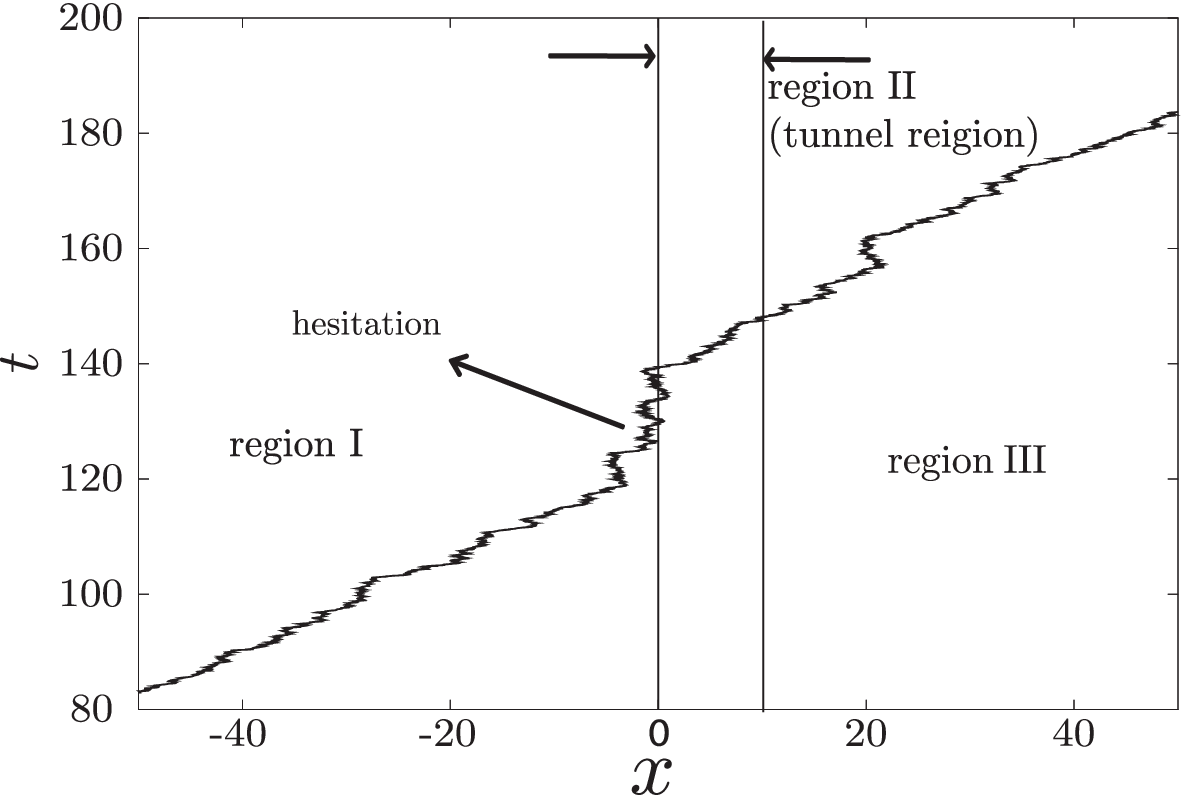
Let us turn to calculate the tunneling time of the BEC wave packet. Figure 3 shows a typical transmission sample path, calculated by Eq.(23) with “backward time evolution method” [18, 19]. The tunneling time is defined as the averaged time interval in which the random variables stay in the barrier region II,
| (34) | |||||
where and are the initial and final times for the scattering problem, respectively. As shown in Fig.3, the random variable of the transmission sample path stays in front of the potential barrier [18]. This hesitating phenomenon is due to a strong interference between the incident and reflecting waves. We define the hesitating time as the averaged time interval in which the random variables pass through some region in front of the potential barrier . The interaction time is also defined as a sum of the tunneling time and the hesitating one . Thus the interaction time represents the passage time through the region .

We study how the interaction strength affects the tunneling time. Figure 4-(a) shows a the behavior of the tunneling time versus . We can see that the tunneling time decreases as increases. The nonlinear repulsive interaction accelerates the motion of the BEC wave packet in the potential region. Figure 4-(b) shows the behavior of the tunneling time versus the potential height. The tunneling time with increases first as the potential becomes higher, which can be understood intuitively, but shifts to a decrease for the high potential. The latter behavior can be explained by the Büttiker-Landauer time , which is also obtained by the Nelson stochastic approach for high and wide potential barrier with [18]. On the other hand, the tunneling time does not vary much with the potential height in case of the strong interaction, and approaches to a constant value. Our results imply that the tunneling time of the BEC wave packet mainly depends on the interaction strength , but not on the potential height.
To explain the independence of the tunnneling time for large , we take a simple model of BECs in a double well potential. We suppose that two BECs are initially in a stationary state with the condensate particle number difference and the phase difference . Then, we add particles to the left well, , and this number difference induces the tunnel current form the left well to the right one. Then the motion of the BECs between the two wells are described by the simultaneous equations [28]
| (39) | |||
| (40) |
where , , and represent the total condensate particle number, the tunnel coefficient, and the interaction constant, respectively. It is assumed in derivation of Eqs.(39) and (40) that and are small. Their solutions are given by
| (41) | |||||
| (42) |
with the frequency . Since we are not interested in an oscillation of the two BECs here but only in the tunneling from the left to the right, we consider only for and ignore the order . Then, we obtain
| (43) |
The phase difference corresponds to the tunneling current velocity, so larger implies smaller tunneling time. One notices the following two features of the phase difference . First, it increases monotonically as does. Second, while it depends on in the weak interaction limit , it becomes independent in the strong interaction limit . As and in the toy model with the double well can be identified with and the potential height in the model of the potential barrier, respectively, the arguments just above explain the behaviors of the tunneling time in Fig.4 .


Finally, we investigate the properties of the hesitating and interaction times versus the potential width , which are shown in Fig.5. For , while the tunneling time increases monotonically, the hesitating time decreases for large . This is because that the particle of the transmission sample path for thick potential tends to have higher velocity and therefore to pass through the region in front of the potential barrier faster [29]. As becomes larger, the tunneling and hesitating times decrease. One can see that the hesitating time is affected by the interaction strength much more than the tunneling time, as in Fig.5. This result can be explained as follows: The incident and reflecting waves make a strong interference in front of the potential barrier and create the high density region. There the non-linear repulsive interaction term contributes strongly to the behavior of the sample path. Next, we refer to the dependence of the interaction time on , as in Fig.6 . It is predicted, based on the method of phase time [7], that the “tunneling time” for thick-enough barrier becomes independent of the barrier length for non-interacting systems, which is known as the Hartman effect. In the Nelson’s stochastic approach, the tunneling time with grows but the hesitating time decreases, and their sum, the interaction time, seems to approach to a constant value, as in Fig.6. This corresponds to the Hartman effect in Nelson’s stochastic approach. We remark that the Hartman effect is apparently violated in the presence of the nonlinear interaction, . The violation of the Hartman effect for non-linear interaction has also been pointed out in Ref. [22] .
IV Arrival Time of the BEC Wave Packet
As seen in Fig.1-(b) , the center momentum for the transmitted wave packet becomes larger than that for the incident one. In tunneling process, the non-linear interaction reduces the tunneling and hesitating times. The acceleration of the quantum particle in the presence of the potential barrier and nonlinear interaction accounts for these results. In this section, we investigate the acceleration of the wave packet in view of the mean arrival time [29].
Introduce the arrival time distribution at the position as
| (44) |
and the mean arrival time as
| (45) |
One can calculate the difference between the mean arrival times with and without a potential barrier,
| (46) |
Due to the nonlinear interaction, the center of the momentum for the transmitted wave packet becomes large in Fig.1-(b) and the mean arrival time should reflect this effect. In order to study the acceleration of the BEC wave packet in the potential barrier, we focus on the mean arrival time at the potential barrier edge .

The results of are shown in Fig.7-(a) . At first, we see that can become negative and that the non-linear interaction gives rise to a large , which strongly suggests a big acceleration inside the potential barrier region. For comparison, we also show the difference between the interaction times with a potential barrier and without it in Fig.7-(b) . The difference becomes small as the interaction strength goes up, but does not become negative in contrast to . It indicates that the velocity of the transmitted wave packet does not exceed that of the free wave packet. Although the above results sound paradoxical at first glance, the Nelson’s method can reproduce physical quantities in quantum mechanics and the arrival time distribution can actually be obtained from the transmitted sample paths (Fig.8).


The key to understand these results is a displacement of the peak position of the wave packet. Figure 9-(a) shows the wave packets at . It tells us that before the peak of the incident wave packets reaches the potential barrier the peak of the transmitted one appears at . Furthermore, only the front part of the incident wave packet seems to contribute to the transmission. This situation becomes clear in the Nelson’s stochastic interpretation. From the transmitted and reflected sample paths, we can construct the probability distributions for the respective components. Figure 9 shows that the transmitted wave packet is constructed mainly from the front part of the incident wave packet. As a result, a displacement of the peak position of the wave packet occurs and it looks like its large acceleration. This mechanism is similar to the superluminal tunneling of the photon [30, 31]. We point out the strong dependence of the displacement on the interaction strength.
V Summary
In this paper, we have investigated the times related to the tunnneling of the BEC wave packet in the Nelson’s stochastic approach. There are the three times, namely the tunneling time for which a particle is in a potential barrier, the hesitating one for which it stays in front of the barrier and the interaction one, give by a sum of the tunnneling and hesitating times. Applying the mean field approach to the Nelson’s stochastic formulation, we derive the GP equation directly.
According to the stochastic formulation, we have performed numerical calculations. First, it is found that the tunneling time decreases as the interatomic repulsive interaction becomes stronger and is not affected so much by the potential barrier height for the strong interaction. The dependence of the hesitating and interaction times on the parameters, especially on the interaction strength, has been revealed. It is seen that the Hartman effect is violated when the non-linear interaction is switched on.
We have also calculated the mean arrival time of the BEC wave packet and have seen a large displacement of its peak position. This result implies that it is not adequate to define the tunneling time by the peak motion ( or the group velocity ) of the BEC wave packet.
Acknowledgements.
One of the author (K. K.) would like to thank Dr. M. Okumura for a fruitful discussion.References
- [1] N. H. Anderson, J. R. Ensher, M. R. Matthews, C. E. Wieman, and E. A. Cornell, Science. 269, 198 (1995).
- [2] K. B. Davis, M.-O. Mewes, M. R. Andrews, N. J. van Druten, D. S. Durfee, D. M. Kurn, and W. Ketterle, Phys. Rev. Lett. 75, 3969 (1995).
- [3] W. Ketterle, D. S. Durfee, and D. M. Stamper-Kurn. in Bose-Einstein Condensation in Atomic Gases, edited by M. Inguscio, S. Stringari, and C. E. Wieman, (IOS Press, Amsterdam, 1999).
- [4] G. J. Milburn, J. Corney, E. M. Weight, and D. F. Walls, Phys. Rev. A 55, 4318 (1997).
- [5] A. Smerzi, S. Fantoni, S. Giovanazzi, and S. R. Shenoy, Phys. Rev. Lett. 79, 4950 (1997).
- [6] G. Dekel and V. Fleurov, Phys. Rev. A 75, 043617 (2007).
- [7] T. E. Hartman, J. Appl. Phys. 33, 3427 (1962).
- [8] A. I. Baz’, Sov. J. Nucl. Phys. 4, 182 (1967).
- [9] A. I. Baz’, Sov. J. Nucl. Phys. 5, 161 (1967).
- [10] M. Büttiker, Phys. Rev. B 24, 6178 (1983).
- [11] M. Büttiker and R. Landauer, Phys. Rev. Lett. 49, 1739 (1982).
- [12] M. Büttiker, Phys. Scr. 32, 429 (1985).
- [13] Th. Martin and R. Landauer, Phys. Rev. A 47, 2023 (1993).
- [14] C.R. Leavens, Phys. Lett. A 178, 27 (1993).
- [15] W.R. McKinnon and C.R. Leavens, Phys. Rev. A 51, 2748 (1995).
- [16] D. Sokolovski and L. Baskin, Phys. Rev. A 36, 4604 (1987).
- [17] N. Yamada, Phys. Rev. Lett. 83, 3350 (1987).
- [18] K. Imafuku, I. Ohba, and Y. Yamanaka, Phys. Lett. A 204, 329 (1995).
- [19] K. Imafuku, I. Ohba, and Y. Yamanaka, Phys. Rev. A 56, 1142 (1996).
- [20] K. Hara and I. Ohba, Phys. Rev. A 62, 032104 (2000).
- [21] K. Hara and I. Ohba, Phys. Rev. A 67, 052105 (2000).
- [22] Z. Duan, B. Fan, C. Yuan, J. Cheng, S. Zhu, and W. Zhang, Phys. Rev. A 81, 055602 (2010).
- [23] E. Nelson, Phys. Rev. 150, 1079 (1966).
- [24] E. Nelson, Quantum Fluctuations, (Princeton Univ. Press, New Jersey, 1985).
- [25] B. M. Deb and P. K. Chattaraj, Phys. Rev. A 39, 4 (1989).
- [26] A. B. Nassar, Phys. Rev. A 33, 5 (1986).
- [27] M. I. Loffredo and L. M. Morato, J. Phys. A: Math. Theor. 40, 8709 (2007).
- [28] C. J. Pethick and H. Smith, Bose-Einstein Condensation in Dilute Gases Second Edition , (Cambridge University Press, Cambridge, 2008).
- [29] K. Aoki, A. Horikoshi, and E. Nakamura, Phys. Rev. A 62, 022101 (2000).
- [30] A. M. Steinberg, P. G. Kwiat, and R. Y. Chiao, Phys. Rev. Lett. 71, 5 (1993).
- [31] M. Tanaka, M. Fujiwara, and H. Ikegami, Phys. Rev. A 34, 6 (1986).