Distributed Stochastic Power Control in Ad-hoc Networks: A Nonconvex Case

We consider an ad-hoc wireless network with a set $\mathcal{L}=\{1,...,L\}$ of links, where the channel is interference-limited, and all $L$ links treat interference as noise, as illustrated in Fig. 1. Such a model of communication is also applicable to cellular networks [2]. Each link consists of a dedicated transmitter-receiver pair.¹¹ 1 We use the terms “user” and “link” interchangeably throughout. We denote by $h_{lk}$ the fixed channel gain between user $l$’s transmitter and user $k$’s receiver, and by $p_{l}$ the transmission power of link $l$ with $P_{l}^{\max}$ being its maximum power constraint. For static channels, the received SINR for the $l$th user with a matched filter receiver is given by

where $\mathbf{p}=(p_{1},...,p_{L})$ is a vector of the users’ transmission powers and $n_{l}$ is the noise power. Accordingly, the $l$th user receives the utility $U_{l}(\gamma_{l})$, where $U_{l}(\cdot)$ is continuous and strictly increasing. We assume that each user $l$’s utility is zero when $\gamma_{l}=0$, i.e., $U_{l}(0)=0$. For ease of reference, some notation is listed in Table I.²² 2 We use bold symbols (e.g., $\mathbf{p}$) to denote vectors and calligraphic symbols (e.g., $\mathcal{L}$) to denote sets.

We seek to find the optimal power allocation $\mathbf{p}^{*}$ that maximizes the overall system utility subject to the individual power constraints, given by the following optimization problem:

In general, (2) is a nonconvex problem³³ 3 For some special utility functions $U_{l}(.)$, (2) can be transformed into a convex problem [4]. In this paper, we focus on the nonconvex case that cannot be transformed to a convex problem by change of variables.. In particular, if the utility function is the Shannon rate achievable over Gaussian flat fading channels, namely $U_{l}(\gamma_{l}(\mathbf{p}))=w_{l}\log(1+\gamma_{l}(\mathbf{p}))$, where $w_{l}>0$ is a weight associated with user $l$, (2) boils down to the weighted sum rate maximization problem, which is known to be nonconvex and NP-hard [6]. Note that the weights can serve as the fairness measures[17] for different scenarios. In particular, in queueing systems, for arrival rates within the stability region, packet queues can be stabilized by solving this weighted sum rate maximization problem, when the instantaneous queue lengths are chosen as the weights. In Section III, we will discuss how to stabilize the packet queues by integrating our distributed power control algorithms with the back-pressure algorithm.

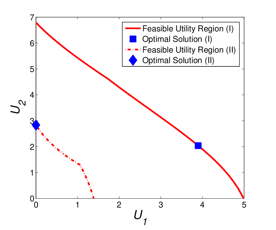
Let $\mathcal{F}$ denote the feasible utility region, where for each point $\mathbf{U}=(U_{1},...,U_{L})$ in $\mathcal{F}$, there exists a power vector $\mathbf{p}$ such that $U_{l}=U_{l}(\gamma_{l}(\mathbf{p}))$ for all $l\in\mathcal{L}$. The feasible utility region $\mathcal{F}$ is nonconvex, and in general, finding the globally optimal solution to (2) in $\mathcal{F}$ is challenging. In the following example, we illustrate the geometry of $\mathcal{F}$ for the utility $U_{l}(\gamma_{l}(\mathbf{p}))=w_{l}\log(1+\gamma_{l}(\mathbf{p}))$ and evaluate the solutions to (2) given by some existing power control approaches discussed in Section I.

Example: For the case with two links, Fig. 2 illustrates the nonconvex feasible utility region $\mathcal{F}$ for different system parameters. We compare the performance of the existing approaches [2, 7, 12, 11] in Table II.

Remarks: The solutions to (2) given by [2, 7, 11] are either distributed but suboptimal or optimal but centralized. In particular, [2] solves (2) by using geometric programming (GP) under the high-SINR assumption, which yields a suboptimal solution to (2) when the assumption does not hold (e.g., this is the case in this example above). The ADP algorithm [7] can guarantee only local optimality⁴⁴ 4 The local optimal solution found by ADP happens to be globally optimal only in one of the cases that are illustrated in Table II. in a distributed manner. The MAPEL algorithm [11] can achieve the globally optimal solutions but it is centralized with high computational complexity. Compared with these algorithms, the SEER algorithm [12] can guarantee global optimality in a distributed manner but message passing needed in each iteration can be demanding, i.e., each link needs the knowledge of the channel gains, the receiver SINR and the signal power of all the other links. It is worth noting that the performance of SEER hinges on the control parameter that can be challenging to choose on the fly.

In order to devise low-complexity distributed algorithms that can guarantee global optimality, we first study the basic properties for the solutions to (2), and then convert (2) into a more structured max-min problem.

In this section, we study algorithms achieving global optimality for (3). First, we propose a centralized algorithm for (3), which will serve as a benchmark for performance comparison. Then, by using EDT and SA, we propose a distributed algorithm, DSPC, for the problem (3). Building on this, we propose an enhanced algorithm EDSPC to improve the convergence rate of DSPC.

1) A Centralized Algorithm

Based on Lemma 2.1 and Lemma 3, we develop a centralized algorithm (Algorithm 1) to solve the max-min optimization problem (3) under consideration. Roughly speaking, by dividing the simplex $\mathcal{S}=\{\mathbf{x}|\sum_{l\in\mathcal{L}}x_{l}=1,0\leq x_{l}\leq 1,\forall l\in\mathcal{L}\}$ into many small simplices, the algorithm can find the optimal point on the boundary of $\mathcal{F}$.

In this section, we evaluate the utility and convergence performance of Algorithms 2 and 3 (DSPC⁹⁹ 9 The geometric cooling schedule is employed to accelerate the convergence rate of DSPC in the simulation. DSPC updates penalty values until they satisfy the threshold-based optimality condition. and EDSPC). We consider a wireless network with six links randomly distributed on a 10m-by-10m square area. The channel gains $h_{lk}$ are equal to $d_{lk}^{-4}$, where $d_{lk}$ represents the distance between the transmitter of user $l$ and the receiver of user $k$. We assume $U_{l}(\gamma_{l}(\mathbf{p}))=\log(1+\gamma_{l}(\mathbf{p}))$, $P_{l}^{\max}=1$ and $n_{l}=10^{-4}$ for all $l\in\mathcal{L}$, and consider one randomly generated realization of channel gains given by

Fig. 4 shows how the total utility in the EDSPC algorithm converges over time, where we choose all the initial penalty values equal to 10. Also, we choose $\xi=0.9$, $\rho=1$ and $\varrho=1$, and use Algorithm 1 as a benchmark to evaluate the optimal performance. As shown in Fig. 4, the EDSPC algorithm approaches the optimal utility, when the initial penalty values are carefully chosen. Moreover, the convergence rate of the EDSPC algorithm is much faster than DSPC, since DSPC continues updating the penalty values after the optimal solution is found for the current penalty values. Fig. 5 illustrates the average performance (with confidence interval) of DSPC, EDSPC, and SEER under 100 random initializations, with the same system parameters as in Fig. 4. As shown in Fig. 5, both DSPC and EDSPC are robust against the initial value variations.

A comparison with the SEER and ADP is also depicted in Fig. 4 and 5. As mentioned in Section I, ADP can only guarantee local optimality. Therefore, for nonconvex problems (e.g., in this example), ADP may converge to a suboptimal solution. As noted in [12], the performance of SEER heavily hinges on the control parameter that can be challenging to choose on the fly. In contrast, DSPC can approach the globally optimal solution regardless of the initial parameter selection, but the convergence rate may be slower. Further, EDSPC improves the convergence rate, but the initial penalty values would impact how close it can approach the optimal point. From the point of view of reducing the amount of message passing, in our algorithms each link does not need any knowledge of the channel gains (including its own channel gain), the receiver SINR of the other links and the signal power of the other links, which are all used in the SEER algorithm.

Consider the same wireless network model with $L$ links as in Section II. We assume that there are $S$ classes of users in the system, and that the traffic brought by users of class $s$ follows $\{A_{sl}(t)\}_{t=1}^{\infty}$, which are i.i.d. sequences of random variables for all $l=1,...,L$ and $s=1,...,S$, where $A_{sl}(t)$ denotes the amount of traffic generated by users of class $s$ that enters the link $l$ in slot $t$. Let $Q_{T(l)}^{s}(t)$ and $Q_{R(l)}^{s}(t)$ denote the current backlog in the queue of class $s$ in slot $t$ on the transmitter and receiver sides of link $l$, respectively. The queue length $Q_{T(l)}^{s}(t)$ evolves over time as

where $r_{l}^{s}(t)$ denotes the transmission rate of link $l$ for users of class $s$. The third term in (10) denotes the traffic from the other links. Assuming that the second moments of the arrival process $\{A_{sl}(t)\}_{t=1}^{\infty}$ are finite, the queue length process $\{Q_{T(l)}^{s}(t)\}_{t=1}^{\infty}$ forms a Markov chain.

Let $E_{sl}=1$ be the indicator that the path of users of class $s$ uses link $l$, and $E_{sl}=0$, otherwise. As is standard [21, 22, 23], the stability region is defined as follows.

For the sake of comparison, the throughput region¹⁰¹⁰ 10 Note that the feasible utility region $\mathcal{F}$ defined in Section II is the throughput region, when the utility function is the same as the rate function. $\mathcal{F}$ of the corresponding saturated case is defined as the set of all feasible link rates, i.e., $\mathcal{F}=\{\mathbf{r}|r_{l}=r_{l}(\mathbf{p}),\mathbf{p}\in\mathcal{P}\}$. In general, the throughput region $\mathcal{F}$ may be different from the stability region $\Lambda$, except for some special cases (e.g., in slotted ALOHA systems the throughput region and the stability region are the same [28] for two links and in a multiple-access channel the information theoretic capacity region is equivalent to its stability region [29]).

The system is stable if the arrival rates of packet queues are less than the service rates such that the queue lengths do not grow to infinity. In order to stabilize packet queues, it is critical to find the optimal scheduling and power allocation policy that maximizes the weighted sum rate given by (11). By integrating our power control algorithms and the back-pressure algorithm, we propose the following joint scheduling and power allocation policy (presented in Algorithm 4) to stabilize the queueing system.

The proof is similar to that in [23, 24], and is omitted for brevity.

Note that Algorithm 4 can be viewed as a single-hop dynamic back-pressure and resource allocation policy [24], crafted towards solving the weighted sum rate maximization problem (11). Specifically, by using the DSPC algorithm, Algorithm 4 can be implemented distributively to find the globally optimal resource allocation. We should caution that EDSPC can be applied to improve the convergence rate of Stage 2 in Algorithm 4 but it may render a suboptimal schedule (i.e., it can not stabilize all possible $\{\psi_{s}\}_{s=1}^{S}$ within $\Lambda$), due to the fact that EDSPC may not always find the global optimal power allocation.

To reduce the complexity, we can consider a policy that computes (11) every few slots, and it can be shown that this policy can also stabilize the system, when $\{\psi_{s}\}_{s=1}^{S}$ is strictly interior to the stability region $\Lambda$ [26, 27].

In this section, we present numerical results to illustrate the use of Algorithm 4 for stabilizing a queueing system. We consider a one-hop network (i.e., $\mathbf{E}=\{E_{sl}\}$ is the identity matrix) with two users (classes), where the channel gains are given by $h_{11}=0.3$, $h_{12}=0.5$, $h_{21}=0.03$, and $h_{22}=0.8$, and the noise power is 0.1 for each link. The maximum transmission power is set to 1 and 2 for links 1 and 2, respectively. Besides, we assume that the users of class $s$ arrive at the network according to a Poisson process with rate $\lambda_{s}$, and that the size of file brought by each user follows an exponential distribution with mean $\nu_{s}$. The load brought by users of class $s$ is then $\psi_{s}=\lambda_{s}\nu_{s}$. For this example, we also study the stability region $\Lambda$ and compare it with the throughput region $\mathcal{F}$ of the corresponding saturated case as illustrated in Fig. 6. The stability region follows from the union of link rates that are conditioned on whether the other link is backlogged or not [28, 29]. First, we derive the stability region for the given power allocation. Then, we vary power allocation in the feasible region, and by taking the envelope of these regions, we obtain the overall stability region shown in Fig. 6. However, different from the previous cases, where the throughput region is the same as the stability region, e.g., in a slotted ALOHA system with two links [28] and in a multiple-access channel [29], in our case under the SINR model, the throughput region $\mathcal{F}$ is strictly smaller than the stability region (due to the underlying nonconvex optimization problem), as observed from Fig. 6, which is the convex hull of $\mathcal{F}$, i.e., $Co(\mathcal{F})$, achievable by timesharing across different transmission modes¹¹¹¹ 11 The transmission mode is defined as the transmission rate pair within the throughput region $\mathcal{F}$..

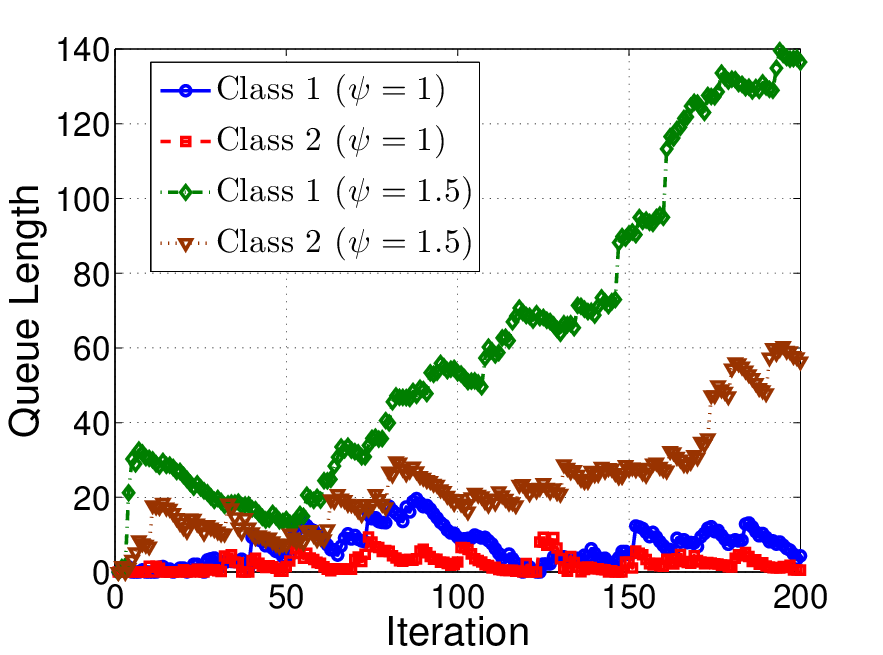
Then, we vary the arrival rate $\lambda$ and the average file size $\nu$ to change the traffic intensity $\psi=\lambda\nu$. Assuming that the arrival rate and the average file size of each user are the same, we compare the sample paths of each user’s queue length for $\psi=1$ ($\lambda=1$, $\nu=1$) with $\psi=1.5$ ($\lambda=1.5$, $\nu=1$) in Fig. 7. When $\psi=1$, which falls in the stability region shown in Fig. 6, the system is stabilized by using Algorithm 4, while, when $\psi=1.5$, which is outside the stability region, the system becomes unstable. Fig. 8 illustrates the average delay of the system as a function of the arrival rates. The delay is finite for small loads and grows unbounded when the loads are outside the stability region.

Beyond the model described in Section II, we consider that each user $l$ has one transmitter and a set $\mathcal{M}_{l}$ of receivers. The corresponding transmission rate, $r_{l}$, is determined by the bottleneck link among these transmitter-receiver pairs, i.e., $r_{l}=\min_{m\in\mathcal{M}_{l}}r_{lm}$, where $r_{lm}$ denotes the link rate between the transmitter of user $l$ and its receiver $m$, and it is calculated based on the Shannon rate $\log(1+\gamma_{lm}(\mathbf{p}))$ for Gaussian, flat fading channels. Here, we do not consider the general broadcast capacity region but rather focus on maximizing the bottleneck link rates.

We seek to find the optimal power allocation $\mathbf{p}^{*}$ that maximizes the overall system utility subject to the power constraints in multicast communications, as follows:

Similar to (2), (12) is nonconvex due to the complicated interference coupling between individual links. In order to devise distributed algorithms to solve (12), it suffices to relax $r_{l}=\min_{m\in\mathcal{M}_{l}}r_{lm}$ in (12) as $r_{l}\leq\log(1+\gamma_{lm}(\mathbf{p})),\forall~l\in\mathcal{L},m\in\mathcal{M}_{l}$. Thus, (12) can be rewritten as

We develop next distributed algorithms that can find the globally optimal solutions to (13) based on EDT and SA. To this end, we first rewrite the optimization problem (13) as

Next, we use EDT to write Lagrangian for (14) as

where $\alpha_{lm}\in\mathbb{R}$ are the penalty multipliers. Based on EDT, there exist finite $\alpha_{lm}^{*}\geq 0$ for all $l\in\mathcal{L},m\in\mathcal{M}_{l}$ such that, for any $\alpha_{lm}>\alpha_{lm}^{*}$, $\forall~l\in\mathcal{L},m\in\mathcal{M}_{l}$, the solution to (15) is the same as (14) [14]. Since there is no coupling among the power constraints of the individual users, (15) does not include the power constraints. Thus, each user satisfies its own power constraint while minimizing (15) in a distributed operation.

As in Section II, the key step is to let each user perform a local stochastic search based on SA. Let $r_{l}$ and $p_{l}$ denote the primal values of the $l$th user, and $r_{l}^{\prime}$ denote the new values randomly chosen by the $l$th user, which is treated as a new target transmission rate for the $l$th user. Different from the unicast communications case, the $l$th user updates $p_{l}^{\prime}$ by

where $\gamma_{lm}$ is the current SINR measured at the receiver $m$ of user $l$. Note that (16) does not need any information of the channel gains except the SINR feedback from the intended receivers, i.e., $\gamma_{lm}$. Since (16) is in standard form as described in [19], it converges geometrically fast to the target utility. The steps to update $r_{l}$ and $\alpha_{lm}$ are similar to DSPC Algorithm 2 in Section II. A detailed description of DSPC algorithm for multicast communications is presented in Algorithm 5.

In this section, we evaluate the performance of Algorithms 5 and 6 for multicast communications. We consider a wireless network with four transmitters and each transmitter has two receivers. These transmitters and receivers are randomly placed in a 10m-by-10m square area. The channel gains $h_{lm}$ are equal to $d_{lm}^{-4}$, where $d_{lm}$ represents the distance between the transmitter $l$ and the receiver $m$. The channel gains $h_{lm}$ are equal to $d_{lm}^{-4}$, where $d_{lm}$ represents the distance between the transmitter $l$ and the receiver $m$. We assume $U_{l}(r_{l})=r_{l}$, $P_{l}^{\max}=1$, and $n_{lm}=10^{-4}$ for all $l\in\mathcal{L}$ and $m\in\mathcal{M}_{l}$. Fig. 9 illustrates the fast convergence performance of Algorithms 5 and 6 in multicast communications.¹²¹² 12 The other existing algorithms have been specifically designed for unicast communications; therefore, they are excluded here from the performance comparison. Besides, we examine the average performance (with confidence interval) of DSPC and EDSPC for multicast communications under 100 random initializations with the same system parameters as in Fig. 9. As illustrated in Fig. 10, both algorithms 5 and 6 are robust against the initial value variations.

References

- [1] L. Yang, Y. E. Sagduyu, J. Zhang, and J. H. Li, “Distributed power control for ad-hoc communications via stochastic nonconvex utility optimization,” Proc. IEEE ICC, 2011.
- [2] M. Chiang, P. Hande, T. Lan, and C. W. Tan, “Power control in wireless cellular networks,” Foundations and Trends in Networking, vol. 2, no. 4, pp. 381-553, 2008.
- [3] D. Julian, M. Chiang, D. O. Neill, and S. Boyd, “Qos and fairness constrained convex optimization of resource allocation for wireless cellular and ad hoc networks,” Proc. IEEE INFOCOM, 2002.
- [4] M. Chiang, C. W. Tan, D. Palomar, D. O. Neill, and D. Julian, “Power control by geometric programming,” IEEE Trans. Wireless Commun., vol. 1, no. 7, pp. 2640-2651, 2007.
- [5] M. Xiao, N. B. Shroff, and E. K. P. Chong, “A utility-based power control scheme in wireless cellular systems,” IEEE/ACM Trans. Netw., vol. 11, no. 2, pp. 210-221, 2003.
- [6] Z.-Q. Luo and S. Zhang, “Dynamic spectrum management: complexity and duality,” IEEE J. Sel. Topics Signal Process., vol. 2, no. 1, pp. 57-73, 2008.
- [7] J. Huang, R. Berry, and M. Honig, “Distributed interference compensation for wireless networks,” IEEE J. Sel. Areas Commun., vol. 24, no. 5, pp. 1074-1084, 2006.
- [8] P. Hande, S. Rangan, M. Chiang, and X. Wu, “Distributed uplink power control for optimal SIR assignment in celluar data networks,” IEEE/ACM Trans. Netw., vol. 16, no. 6, pp. 1420-1433, 2008.
- [9] C. U. Saraydar, N. B. Mandayam, D. J. Goodman, “Efficient power control via pricing in wireless data networks,” IEEE Trans. Commun., vol. 50, no. 2, pp. 291-303, 2002.
- [10] T. Alpcan, T. Basar, R. Srikant, and E. Altman, “CDMA uplink power control as a noncooperative game,” Wireless Networks, vol. 8, no. 6, pp. 659-670, 2002.
- [11] L. Qian, Y. J. Zhang, and J. W. Huang, “MAPEL: achieving global optimality for a non-convex power control problem,” IEEE Trans. Wireless Commun., vol. 8, no. 3, pp. 1553-1563, 2009.
- [12] L. Qian, Y. J. Zhang, and M. Chiang, “Globally optimal distributed power control for nonconcave utility maximization,” Proc. IEEE GLOBECOM, 2010.
- [13] S. Geman and D. Geman, “Stochastic relaxation, Gibbs distributions, and the Bayesian restoration of images,” IEEE Trans. Pattern Anal. Mach. Intell., vol. 6, no. 6, pp. 721-741, 1984.
- [14] Y. Chen and M. Chen, “Extended duality for nonlinear programming,” Comput. Optim. Appl., vol. 47, no. 1, pp. 33-59, 2010.
- [15] S. Kirkpatrick, C. D. Gelatt, and J. M. P. Vecchi, “Optimization by simulated annealing,” Science, vol. 220, no. 4598, pp. 671-680, 1983.
- [16] J. E. Wieselthier, G. D. Nguyen, and A. Ephremides, “On construction of energy-efficient broadcast and multicast trees in wireless networks,” Proc. IEEE INFOCOM, 2000.
- [17] J. Mo and J. Walrand, “Fair end-to-end window-based congestion control,” IEEE/ACM Trans. Netw., vol. 8, no. 5, pp. 556-567, 2000.
- [18] S. Boyd and L. Vandenberghe, Convex Optimization. Cambridge, U.K.: Cambridge Univ. Press, 2004.
- [19] R. D. Yates, “A framework for uplink power control in cellular radio systems,” IEEE J. Sel. Areas Commun., vol. 13, no. 7, pp. 1341-1347, 1995.
- [20] B. Hajek, “Cooling schedules for optimal annealing,” Math. Oper. Res., vol. 13, no. 2, pp. 311-329, 1988.
- [21] X. Lin, N. B. Shroff, and R. Srikant, “On the connection-level stability of congestion-controlled communication networks,” IEEE Trans. Inf. Theory, vol. 54, no. 5, pp. 2317-2338, 2008.
- [22] L. Tassiulas and A. Ephremides, “Stability properties of constrained queueing systems and scheduling policies for maximum throughput in multihop radio networks,” IEEE Trans. Autom. Control, vol. 37, no. 12, pp. 1936-1948, 1992.
- [23] M. J. Neely, E. Modiano, and C. E. Rohrs, “Dynamic power allocation and routing for time varying wireless networks,” IEEE J. Sel. Areas Commun., vol. 23, no. 1, pp. 89-103, 2005.
- [24] L. Georgiadis, M. J. Neely, L. Tassiulas, “Resource allocation and cross-layer control in wireless networks,” Foundations and Trends in Networking, vol. 1, no. 1, pp. 1-149, 2006.
- [25] H.-W. Lee, E. Modiano, and L. B. Le, “Distributed throughput maximization in wireless networks via random power allocation,” IEEE Trans. Mobile Comput., 2011.
- [26] P. Chaporkar, S. Sarkar, “Stable scheduling policies for maximizing throughput in generalized constrained queueing systems,” IEEE Trans. Autom. Control, vol. 53, no. 8, pp. 1913-1931, 2008.
- [27] Y. Yi and J. Zhang and M. Chiang, “Delay and effective throughput of wireless scheduling in heavy traffic regimes: vacation model for complexity,” Proc. ACM Mobihoc, 2009.
- [28] R. Rao and A. Ephremides, “On the stability of interacting queues in a multiple-access system,” IEEE Trans. Inform. Theory, vol. 34, no. 5, pp. 918-930, 1988.
- [29] A. ParandehGheibi, M. Medard, A. Ozdaglar, A. Eryilmaz, “Information theory vs. queueing theory for resource allocation in multiple access channels,” Proc. IEEE Pers. Ind. Mob. Radio Commun., 2008.