CERN-PH-TH/2010-120
Measuring the W-Boson mass at a hadron collider:
a study of phase-space singularity methods
Abstract
The traditional method to measure the Boson mass at a hadron collider (more precisely, its ratio to the boson mass) utilizes the distributions of three variables in events where the decays into an electron or a muon: the charged lepton transverse momentum, the missing transverse energy and the transverse mass of the lepton pair. We study the putative advantages of the additional measurement of a fourth variable: an improved phase space singularity mass. This variable is statistically optimal, and simultaneously exploits the longitudinal- and transverse-momentum distributions of the charged lepton. Though the process we discuss is one of the simplest realistic ones involving just one unobservable particle, it is fairly nontrivial and constitutes a good “training” example for the scrutiny of phenomena involving invisible objects. Our graphical analysis of the phase space is akin to that of a Dalitz plot, extended to such processes.
I Prolegomena
Neutrinos –and perhaps novel weakly-interacting particles– escape unobserved from the collisions in which they are produced. In the corresponding “missing energy” events, the reconstruction of the masses of the parent particles and the specification of the underlying process are challenging because there are typically fewer kinematical constraints than unknowns. At a hadron collider this situation is rendered even thornier, since particles produced at small angles also escape undetected. This prohibits the determination of the longitudinal momentum of the center of mass system of the colliding partons.
The above limitations confer a higher standing to observables exclusively dependent on transverse momenta [1], or otherwise invariant under longitudinal boosts [2]. In principle, transverse observables are insensitive to the significant uncertainties associated with the (longitudinal) parton distribution functions (pdfs). In practice the uncertainties are to some extent reintroduced via the angular coverage limitations of an actual experiment, which are not invariant under longitudinal boosts.
The quintessential transverse observable is the transverse mass, of -discovery fame. In an event at a hadron collider, consider the production of a single , followed by its decay , with an electron, a muon, or one of their antiparticles. Denote by and the neutrino and charged lepton fourmomenta, respectively. Here and are the momenta of the leptons in the plane transverse to the beam direction(s), and the analogous quantity for the observed final state hadrons. The traditional “transverse mass”, a function of and , whose distribution is used to infer the boson mass, is [1]
| (1) |
where is the angle between the transverse lepton directions. The most precise determination of the mass of the by a single experiment is the one by D [3]. In spite of the relatively unfavorable environment of a hadron collider, its large statistics results in a value with an overall error smaller than that of the LEP experiments. The D result is based on the decays , and the measurement of three highly correlated transverse observables: the traditional “transverse mass” function [1], the lepton’s transverse energy and the total missing transverse energy. The result:
| (2) |
stems from an actual measurement of . But was determined with exquisite precision at LEP. The PDG quotes GeV [4].
The procedure to extract from the distributions in transverse mass, lepton momentum and total missing energy is as follows. A finely spaced set of input boson masses, , is used to generate a set of “templates”: the “Monte Carlo” (MC) expectations for the observed distributions, with all their experimental cuts, estimated uncertainties, calorimeter responses, etc. The values for the comparison of data and expectations are fit to a quadratic form, from whose minimum and width and its estimated error are inferred. Naturally, all the procedure is tested and calibrated by the observed -production and leptonic decay (into , in the D case).
In order of decreasing incidence on the error in Eq. (2), the limitations are the electron’s energy calibration, the uncertainties on the pdfs, and the statistics. For this particular measurement, the backgrounds are well understood and quite negligible.
Given the large statistics already gathered at the Tevatron collider, and with the advent of the LHC as a high statistics precision physics tool, the main limitation of a hadron collider determination of the mass from its decays into electrons and muons is likely to be the pdf uncertainty. At the LHC this problem is in particular exacerbated [5] by the fact that it is a , not a collider, and the quark pdfs in a proton –or the identical antiquark pdfs in an antiproton– are much better known than the antiquark pdfs in a proton.
II Introduction
A ginormous amount of attention has been paid to hypothetical processes involving neutral, long-lived, weakly-interacting final state particles that can only be indirectly detected. A prototypical example is the pair production of squarks followed by their decays into quark plus neutralino. Such processes generally involve two or more particles of unknown masses.
The first aim in the missing particle searches for physics beyond the Standard Model is the establishment or the exclusion of a signal, both tantamount to an efficient suppression of backgrounds. Some novel longitudinal boost invariant variables are a very good choice in this endeavor [2], as demonstrated by the data analysis in [6].
A longer range aim is the measurement of unknown masses, when there are more than one and a candidate process is selected. In this connection, a very general algebraic singularity method has been advocated [7], involving the use of a “singularity variable” (SV), allegedly more powerful than that of a singularity “condition” (SC), such as the one leading, as we shall see, to the result of Eq. (1).
It is too late to discover the , though not to attempt to measure its mass even better, a relevant task in checking the consistency of the Standard Model and constraining the mass of its hypothetical scalar. With this ab-initio motivation, we have exhaustively studied the phase space for production and leptonic decay, a simple undertaking analogous to the analysis of a Dalitz plot, but with incomplete kinematical information (§IV).
We have also studied the singularities of this phase space, and their use in constraining the mass (§IV and V) . We identify the criterion for the theoretically optimal SV and derive its explicit form (§VI, VIII and X). En passant, we find that other nonoptimal SVs, such as the one proposed in [7], are “dangerous”, in that their distributions display fake singularities (§VII).
The singularity variables we study involve the measured longitudinal momentum of the charged lepton, . This longitudinal information is obviously additive to the transverse information exploited in observables such as , but is highly correlated with it (§IX). The distribution directly reflects the pdfs of merging quarks and antiquarks of different flavor. Recent progress in QCD fits and in calculations well beyond the leading order allows one to hope that –eventually– the dominant limitations concerning the problem at hand will not be the theoretical pdf uncertainties, but the limited calorimetric resolutions.
Given a trustable set of pdfs, one can simulate the observable distribution of events for a set of input trial masses and contrast it with observation. This comparison involves the five relevant variables and their correlations; it has no statistically superior competitor. Why then study any alternatives? Besides the pleasure of understanding with use of one’s own neural network, there is the motivation of paving the way of searches for other processes involving unobservable particles, for which it is a-priori prohibitive to simulate all possibilities.
In this note we report on a thorough theoretical study of the extraction of phase space information from single- signal events, but we use the standard model of production and decay only to leading order. We entirely ignore the backgrounds, which are well known to be very modest for this particular process. A reason for these choices is that only the experimentalists themselves can fully model the detector’s effects and backgrounds, and that this modeling is independent from the theoretical issues on which we focus.
III Linguistic quandaries
Based on equations such as , we shall be drawn to give a plethora of meanings to what is, for starters, simply a letter: . It ends up being everything else. The resemblance to -theory is coincidental.
Naturally, may stand for the physical or measured , as well as for its Lorentzian distribution, when the width is not neglected. But it may also, as in the case of the transverse mass, , be a non-Lorentzian function of other observables.
In analyzing data, one compares them with MC generated distributions that depend on an ensemble of input “trial masses”, for which we reserve the label . A different type of trial masses, which we call , appears in “singularity variables”, which are functions of observable momenta and of . Not to make this complex linguistic heritage hereditary, we label the singularity variables (and not once more “”, as in the function) thereby not introducing new meanings to the symbol or the word “mass”.
IV Single- phase space
The full information relevant to the reconstruction of the mass is embedded in the kinematical equations:
| (3) | |||
| (4) | |||
| (5) | |||
| (6) |
where we have made the approximation for the charged lepton. The equations are incomplete in that the longitudinal momentum, , is unconstrained, precluding a direct determination of the boson mass from a “mass peak”. Is there a systematic way to extract the kinematically most stringent information on ?
To answer this question it is useful to study first the phase space described by Eqs.(3-6) in a simplified case. If the energy and transverse momentum of the observed hadrons could be measured with precision, it would be possible to boost every event to the frame. To (temporarily) simplify the algebra, let us just adopt this constraint. Solve the linear equations to express as functions of . Substitute the result in to obtain the phase space
| (7) | |||
| (8) | |||
| (9) |
It will be useful to consider the two solutions to Eq.(7) in :
| (10) |
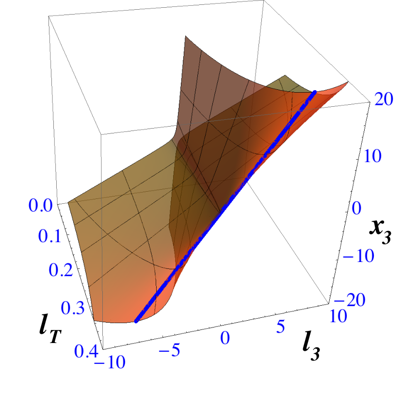
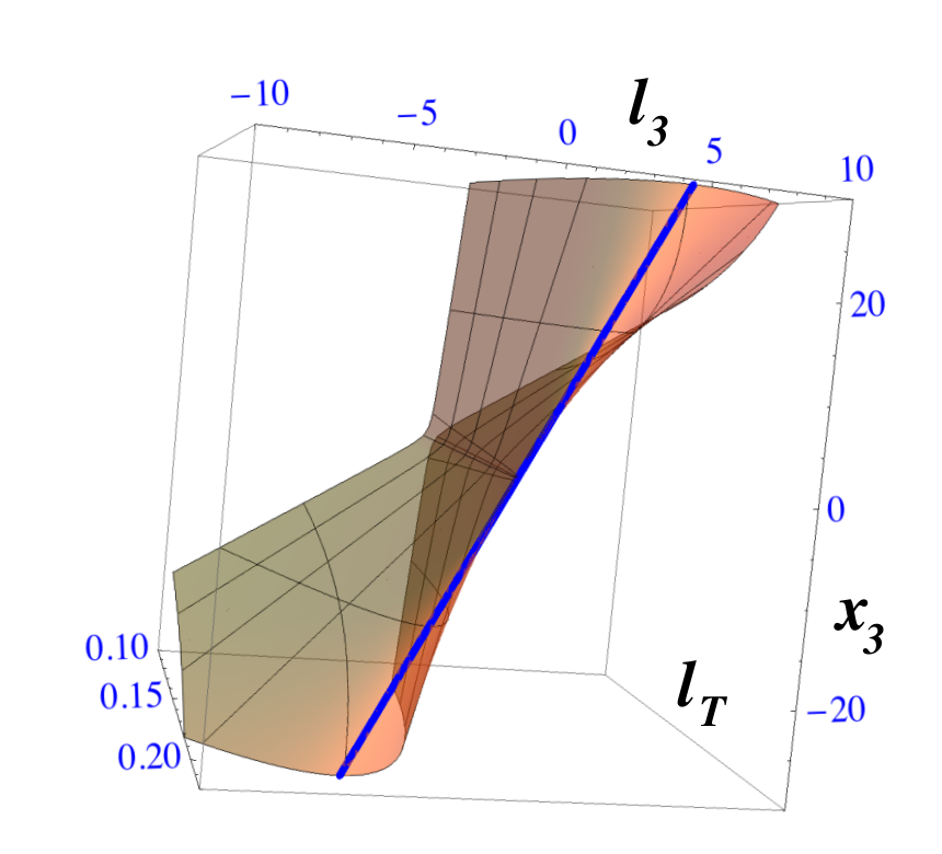
With no loss of generality, and to be able to plot the phase space, do three more things. Take to be positive if directed along the direction of a given (fixed) proton beam. Define the of Eq. (9) to be positive if directed above the beams, negative otherwise. The function , from divers points of view, is plotted in Fig. 1. Along the (blue) straight lines the planes tangent to the phase space contain one “visible” direction, , and the “invisible” direction . The projection of phase space into the visible directions is bounded by the lines .
The boundaries of the phase space projected along an invisible direction onto the space of the visible ones, , are an example of singularity condition(s). At their location there is a single invisible coordinate for fixed values of the visible ones, as opposed to the two of the general case in Eq. (10), and the projected phase space density is not smooth [7].


In practice two cuts have to be applied to the momentum of the observed lepton. We adopt (resulting from a pseudo-rapidity limitation ) and a rather demandingly low GeV. These cuts result in the unobservability of a large fraction of phase space: the (red) domain shown without a mesh in Fig. 2. The maximum happens to be close to the absolute kinematical limit, approximately , at the current LHC energy, TeV. This was probably not the main reason to choose this machine energy.

In simple cases such as the one at hand the singularity condition can be directly obtained. The boundary is the projection of the phase space points at which the tangent plane is vertical and contains the invisible direction . At these points . Eliminating from this expression and Eq. (7) one obtains . At these boundaries .
IV.1 The formal singularity condition
The procedure of the last paragraph requires some guesswork, but can be rendered entirely general and systematic. At a singularity one or more of the invisible directions are contained in the tangent plane to the full phase space. The general condition for this to happen is that, in the space of invisible directions, the row vectors of the Jacobian matrix (with the row index running along the number of equations and the column index over the number of invisible coordinates) be linearly dependent, so that the derivative relative to an -direction normal to these vectors be zero. In other words, at a singularity, the rank of must be smaller than its rank at nonsingular points [7].
IV.2 The function
V Kim’s singularity variable
Discussing the general case with an arbitrary number of invisible final state particles, Kim has argued [7] that the use of a “singularity variable” (SV) is more powerful than that of a singularity “condition” (SC), such as the one leading to the result of Eq. (14).
Kim requires a SV to have four properties [7]:
(i) To vanish at the singularity.
(ii) To be perpendicular –at the singularity– to the phase space surface in the observable
directions.
(iii) To be “normalized such that every event can give the same significance”.
(iv) To be computed to first nontrivial order (the second fundamental
form) in the distance between a phase space
point and the nearest singularity.
Our interpretation of these formal looking choices is the following. Condition (i) is the only scale invariant stipulation. At the singularity, condition (ii) entails a maximal sensitivity to the unknown masses. Condition (iii) ensures that two events with the same distance to the singularity be treated on equal footing. The requirement (iv) is one way to make the procedure general.
To fathom all this it is useful to jump momentarily to the result of Kim’s prescription in our single- case. The SV (more precisely, the singularity function) is:
| (15) |
with as in Eq. (13), and substituted for , as its role will now be that of a trial mass. For this SV reduces to:
| (16) |
Refer for a moment to the limit for the width and a situation with no measurement uncertainties. Consider a set of real or MC generated events, i.e. a list of values of and the histograms of the corresponding values of , for different choices of . For , the real or “MC true” value of the boson mass, the singularity is at , peaks at that point and vanishes for . For a fixed data set and varying , the function varies in shape, but obviously not in statistically useful content. We shall later illustrate these points in detail.
The use of an “implicit” variable may seem to be an overkill. In the single- case with , it is. One could equally well erase in Eq. (16) and use the SV:
| (17) |
which, in conjunction with , embodies two projections of the full distribution .
Contrariwise, one could make the singularity condition into a singularity variable with an implicit :
| (18) |
and consider the distributions . But the information that these distributions contain is precisely the same as that of the distribution , the corresponding histograms are just mirror reflected and shifted relative to one another.
The above unfavorable commentaries on implicit variables are by no means general. Even in the single- case, for , it will not be possible to “erase” from Eq. (15) in the same cavalier spirit in which we erased it from Eq. (16) to obtain Eq. (17). Singularity variables should be of particular practical relevance in problems with more than one unknown mass or unobservable particle, for which the labor of making templates for all possibilities may be out of the question. There, at least at the discovery stage, “clever” variables may be useful to zoom kinematically to the relevant mass ranges before a full analysis is to be contemplated, as discussed in [2].
VI The quest for an optimal variable
It is instructive to consider a trivial example with one visible variable, , and a single invisible one, , constrained by the “Euclidean phase space” equation
| (19) |
This apparently arbitrary instance actually corresponds to an imaginable process, that of a particle decaying into an invisible one, , and a visible one that happens to be at rest. The longitudinal momentum of is and its transverse one, , is measured via the usual transverse balance. is a combination of the masses involved [8].
The value of the unknown quantity in Eq. (19) is encoded in the -distribution. The Jacobian matrix is . The constraint that its rank be reduced is , resulting in the SCs . For a given “observed” , there are two points in . Their nearest singularity is the point , as illustrated in Fig. 3.
Following Kim’s method [7], we obtain for the SV
| (20) |
proportional to the squared (angular or geodesic) to distance measured on the surface. In a less trivial case, the resulting SV would have been the same distance on the quadratic approximation to around .
There is nothing sacred about the elegant result of Eq. (20). There are other SVs that (up to an overall normalization) coincide with to second order. Three examples, illustrated in Fig. 3, are:
- •
(1) The distance between and the hyperplane, , tangent to at (the dotted vertical line, in this case). This distance is the horizontal arrow.
- •
(2) The to distance along the normal direction to at : the slanted arrow.
- •
(3) The square of the length of the vertical arrow.
In the notation of Eq. (20) and normalized so that they coincide with to , these SVs are:
| (21) | |||||
| (22) | |||||
| (23) |
Note that is the 2D analog of the singularity condition used as a SV, as in Eq. (18). That is to say, it is equivalent to the transverse mass distribution.
Is any of these SVs in Eqs. (20) to (23) “the best” in some useful sense? To answer, consider the distributions of the numerical values of the various functions, for fixed (a zero width resonance):
| (24) |
Recalling Eq. (19), and in particle physics language, is the phase space, is the distribution of the values. Monte Carlo generated “diagonal” histograms, , would be the templates for various trial choices of .
In the four cases of Eqs. (20) to (23), with the notation , and normalized to unit integral in the allowed range of the corresponding , the distributions are
| (25) |
In the simple case at hand, one need not refer to “nondiagonal” histograms , that involve the implicit variable . In more blind searches with several unknown masses this may no longer be the case. Moreover the nondiagonal histograms provide one way to ascertain the “goodness” of their SV.
To quantify the amount by which the distribution of a given SV is sensitive to the difference between a “true” mass and a variation thereof, , define the “statistical squared derivative”, , and its integral [9]
| (26) |
The notation reflects the parentage of with the usual measure; it is also the square of the geometrical mean between ordinary and logarithmic derivatives. “Statistical” reflects the fact that is a local measure of a variation relative to the one expected from a standard deviation of 1 size. In this hypothetical case with sharply defined cuts in , is singular at . Regularizing the singularity with a cut we obtain:
| (27) |
The singularities of the different are all and have been equally normalized by construction (and for a fair comparison). The sensitivity to the value of is maximal close to the singularity. This sensitivity puts the SVs of Eqs. (20) to (23) in the “goodness” order
| (28) |
dictated by the second term in brackets in Eqs. (27). The fully “orthogonal” SV is the contest’s winner. The usual transverse mass distribution ( in this simplification) does not fare well.
So far there seems to be no compelling reason not to have made the above variable-comparing analysis with for starters. But in a more realistic case would stand for the central value of a distribution of non zero natural width, while is just an auxiliary quantity introduced for analysis purposes.
To illustrate the above, and to convey the numerical meaning of Eqs. (27), substitute the sharp definition of in Eqs. (19,24) by the one corresponding to a resonance of mass and width :
| (29) |
This corresponds to “spreading” the circle of Fig. (3) and “scanning” it with circles of varying –but sharply defined– , with the help of different “” scanners.
Results for the distributions for Kim’s variable and the orthogonal SV are shown in the upper Fig. (4). The lower figure shows their around the singular point, the domain to which the distributions are most sensitive to the unknown . The figures are drawn for , , showing how the orthogonal is better than . However, the difference is not large and, for a narrow resonance (or one whose width is masked by detector effects) it would be negligible, as the relative differences close to between the of the various SVs diminish linearly as .
The integrals of Eq. (26) over their complete respective kinematical domains are numerically similar, apparently demonstrating that, in toto, all variables are statistically equivalent. In practice this is not the case. The signal-to-noise ratios of the distributions are increasingly unfavorable as one moves away from the neighborhood of the signal’s peak.
We have proven that is better than others, but not that it is the best. Its optimality, however, appears to be intuitively obvious. The phase space of Eq. (19) simply scales as changes. The optimal SV ought to maximize the dependence on at every point in phase space. This dependence is maximal in the direction orthogonal to . The variable measures a distance to the nearest singularity, in that preferred direction.
VII Induced singularities
Let us return to the case of single- production and model the simplified instance as stated in the ending paragraph of §II, that is, to leading order. We use the quark and antiquark parton distribution functions of [10] at an LHC energy of TeV and apply the cuts GeV and to the charged lepton. We ignore the difference between and production.
We choose to present results for the distribution of the values, , of the function:
| (30) |
which differs from Eq. (16) by a factor . This does not affect the arguments to follow. Moreover, in conjunction with the transverse mass () distribution, the use of Eqs. (16) or (30) are equivalent.
A heedless use of Eq. (30) results in an interesting surprise, illustrated in the top panel of Fig. 5. The histogram has two peaks, one of them significantly above the expected singularity at . The peaks fuse as one lets the have its rather narrow width, , as illustrated in the lower panel of Fig. 5. Still, the fused peak is not just the expected singularity at the origin of the SV and the issue calls for understanding.
Consider restricting the phase space of Eqs. (7) and Fig. 1 to its slices at fixed longitudinal momentum of the , , shown in these plots as (green) ellipses (in practice this can only be done at a monochromatic collider). The distribution is shown on the upper Fig. 6, for , . It has two singularities besides the one expected at .
The origin of the singularities is clarified in the lower Fig. 6, where the curve is the phase space , again for , . A uniform distribution of events along , projected on the axis, has three cumulation points at the projections of the vertical tangents. The one at the edge is the expected singularity, the other two are induced singularities. In these units, for there is no induced singularity, for there is one and for there are two. One induced singularity survives the integration over the distribution, as shown in Fig. 5.
The source of the induced singularities is the specific form of the SV in Eq. (30) –or of the formal SV of Eq. (16)– which results in a fixed- phase space the curvature of whose surface is not everywhere of the same sign. The induced singularities are not endpoints, but are event accumulation points for the same reason as the endpoints, i.e. the tangent manifold to the phase space at their locations contains invisible directions.
In a process with just one mass scale to disentangle, the complications we just discussed are a lesser problem. In a process with more than one mass scale, they are a putative source of confusion. The fully orthogonal SV of Eq. (22) does not result in induced singularities.
VIII Results
For the single- case at hand, consider the “fully orthogonal” variable akin to in Eq. (22). We call it and discuss it first in the instance. Its geometrical interpretation is depicted in Fig. (2); is a measure of the length of the arrow, which is orthogonal to a phase space point with coordinates and ends in the plane tangent to the phase space surface at the singularity line.
Define the unit vector orthogonal to the surface of Eq. (7):
| (31) |
The length, , of the orthogonal segment joining with a point in the plane tangent to the singularity is such that
| (32) |
More explicitly
| (33) |
with as in Eq. (10). For each pair (an event) there are two equal probability solutions, the two roots of the equation. In generating events we chose at random the sign in Eq. (10).
We show in Fig. (7) the results for the and distributions. All three graphs are generated for a peak mass of the , . As shown in the bottom figure, for a trial mass the peak of the distribution shifts away from , becoming wider and, for , double peaked: there is for this “bad” choice an induced singularity, even for the optimal SV. Naturally, the histograms with are not statistically independent from the one. While they may be used to “focus” on the correct choice of , the extraction of information on the boson mass would ultimately hinge on a set of templates for values close to its currently measured value.
The value of is not always real. When the value of chosen by the Lorentzian distribution of physical (or MC generated) values of is such that , involves the square root of a negative number. There is nothing pathological about these events. The way to “recover” them is to set:
| (34) |
In the middle Fig. (7), for example, the recovered events are those at .
IX Correlations
It is clear that the transverse mass –or its equivalent of Eq. (18)– and the SV of Eq. (33) are highly correlated. They both vanish at the singularity as . To illustrate the point, define the variable
| (35) |
which has the same mass dimensionality as and, close to the singularity, carries the same information as . The double histogram , shown in Fig. 8, illustrates the expected correlation.

Naturally, correlations between observables constitute a weakness of their ensemble, to which we shall come back in the conclusions. Suffice it to say here that in the “signal only” case at hand, there is only one mass scale to extract from the data: the correlations are unavoidable.
X The general case
In Figs. (1,2) we have profited from the fact that the phase space of Eq. (9) is a function of to plot the phase space for negative and positive . For this is no longer possible. Let and be the moduli of the corresponding vectors and be the angle between them. The general case phase space is then:
| (36) | |||
for which the generalization of the result of Eq. (10) is
| (37) | |||
and that of is
| (38) |
The statistically optimal is computed exactly as in the previous section, with the result:
| (39) |
where is computed as in Eq. (31) in terms of the phase space function of Eq. (36). More explicitly:
| (40) |
Some examples of the general phase space surface are given in Fig. 9.

XI Conclusions and outlook
We have studied in detail the phase space of the simplest interesting hadron collider process involving an unobservable particle and only one mass to be determined. Naturally, the crucial ingredients are the phase space projections onto the observable momenta, their limits, and the distances of actual events from these limits.
The edge of the projected phase space is given by the formal singularity condition, Eq. (12), which can be re-expressed as a function of the observable momenta, Eq. (14) and coincides with the consuetudinary transverse mass function, Eq. (1).
The “singularity variables” are various measures of the distance of an actual event to the nearest edge singularity. We have determined in §VI the measure for which SV is statistically optimal, which we called the “statistical squared derivative” and turns out to be well known to statisticians as the “Fisher information” [9]. The actual result ought to have been obvious for starters: the optimal variable – in Eqs. (33,39)– is orthogonal to the phase space at all points and is thereby most sensitive to the unknown mass, which determines the overall scale of momenta.
Somewhat unexpectedly, singularity variables other than the optimal one develop fake singularities away from the edge singularity at , see Fig. (5), top. The ’s natural width suffices to merge the edge and fake singularities, resulting in a peak at , see Fig. (5), bottom. This is a potential complication in their use as tools to determine the unknown mass(es).
Contrary to the SCs, the SVs depend on longitudinal momenta. In the case of single- production, whether or not they may add significant precision to a measurement of the mass depends on the prior level of understanding of the relevant pdfs [5], a question that we have not tried to investigate. It may well turn out, contrariwise, that the optimal SV, with a value of determined by the transverse observables, is a good tool to constrain the pdfs.
The SVs contain the SC as a factor. This makes them “weak”, in that they are highly correlated to the information contained in the SC, as discussed in §IX. The SVs are functions of an auxiliary mass , and of transverse and longitudinal momenta. Varying as in the lower Fig. (7) is an efficient way to “focus” on the relevant mass scale, particularly for cases with more than one unknown mass [7]. But it does not add to the precision with which the mass(es) may be measured.
Whether or not the various and rather negative conclusions of the previous two paragraphs apply to cases wherein more than one particle decays into invisible ones is a question that we plan to discuss in subsequent work. The answer requires a detailed study of the relevant phase space, akin to the one in this note.
Acknowledgements
We are indebted to Frederik Dydak, Francisco Javier Girón, Ben Gripaios, Cayetano Lopez, Rakhi Mahbubani, Maurizio Pierini, Chris Rogan and Raymond Stora for comments and discussions.
References
- [1] V.D. Barger, A.D. Martin and R.J.N. Phillips, Z. Phys. C 21 (1983) 99; J. Smith, W. L. van Neerven and J. A. M. Vermaseren, Phys. Rev. Lett. 50, 1738 (1983).
- [2] C. Rogan, arXiv:1006.2727.
- [3] V.M. Abazov et al. D collaboration, Phys. Rev. Lett.103:141801 (2009), arXiv:0908.0766v2.
- [4] C. Amsler et al. (Particle Data Group), Phys. Lett. B667, 1 (2008) and 2009 partial update for the 2010 edition (URL: http://pdg.lbl.gov).
- [5] M.W. Krasny et al., Eur.Phys.J. C69:379-397,2010. arXiv:1004.2597 [hep-ex]
- [6] CMS Collaboration, “Inclusive search for squarks and gluinos at TeV”. CMS PAS SUS-10-009 (2011).
- [7] I.W. Kim Phys. Rev. Lett. 104:081601 (2010), arXiv:0910.1149v1.
- [8] B. M. Gripaios, “LHC Mass Measurement, Algebraic Singularities, and the Transverse Mass,” in New Physics at the LHC. Les Houches Report, 2009, arXiv:1005.1229.
- [9] F.J. Girón informs us that our statistical derivative is nothing but the statistician’s “Fisher’s information”.
- [10] http://durpdg.dur.ac.uk/HEPDATA/PDF