跳到论文正文
W Papers独立论文阅读器 arXiv:1106.0321 论文正文 计算阅读时间 · 0%
引用这篇论文根据当前论文元数据生成,正式投稿前建议核对。


License: arXiv.org perpetual non-exclusive license
arXiv:1106.0321v3 [math.ST] 13 Jan 2012

Sparse Non Gaussian Component Analysis by Semidefinite Programming

Elmar Diederichs ††thanks: The author is partially supported by the Laboratory of Structural Methods of Data Analysis in Predictive Modeling, MIPT, through the RF government grant, ag. 11.G34.31.0073. Furthermore the author is grateful for funding to the Competitive Procedure of the Leibniz Association within the ”Pact for Research and Innovation” framework. Affiliation: Weierstrass Institute Affiliation: Mohrenstr. 39, 10117 Berlin, Germany Email: diederic@wias-berlin.de    Anatoli Juditsky Affiliation: LJK, Université J. Fourier, BP 53 38041 Affiliation: Grenoble cedex 9, France Email: juditsky@imag.fr    Arkadi Nemirovski Affiliation: ISyE, Georgia Institute of Technology Affiliation: Atlanta, Georgia 30332, USA Email: nemirovs@isye.gatech.edu    Vladimir Spokoiny Affiliation: Weierstrass Institute and Humboldt University, Affiliation: Mohrenstr. 39, 10117 Berlin, Germany Email: spokoiny@wias-berlin.de
Abstract

Sparse non-Gaussian component analysis (SNGCA) is an unsupervised method of extracting a linear structure from a high dimensional data based on estimating a low-dimensional non-Gaussian data component. In this paper we discuss a new approach to direct estimation of the projector on the target space based on semidefinite programming which improves the method sensitivity to a broad variety of deviations from normality.

We also discuss the procedures which allows to recover the structure when its effective dimension is unknown.
Keywords: dimension reduction, non-Gaussian components analysis, feature extraction
Mathematical Subject Classification: 62G07, 62H25, 62H30, 90C48, 90C90

1 Introduction

Numerous statistical applications are confronted today with the so-called curse of dimensionality (cf. [13, 31]). Using high-dimensional datasets implies an exponential increase of computational effort for many statistical routines, while the data thin out in the local neighborhood of any given point and classical statistical methods become unreliable. When a random phenomenon is observed in the high dimensional space ℝd\,\mathbb{R}^{d}\, the ”intrinsic dimension” mm covering degrees of freedom associated with same features may be much smaller than dd. Then introducing structural assumptions allows to reduce the problem complexity without sacrificing any statistical information [17, 25]. In this study we consider the case where the phenomenon of interest is (approximately) located in a linear subspace ℐ\mathcal{I}. When compared to other approaches which involve construction of nonlinear mappings from the original data space onto the ”subspace of interest”, such that isomaps [29], local-linear embedding [13] or Laplacian eigenmaps [4], a linear mapping appears attractive due to its simplicity — it may be identified with a simple object, the projector Π∗\Pi^{*} from ℝd\mathbb{R}^{d} onto ℐ\mathcal{I}. To find the structure of interest a statistician may seek for the non-Gaussian components of the data distribution, while its Gaussian components, as usual in the statistical literature may be treated as non-informative noise.

Several techniques of estimating the “non-Gaussian subspace” have been proposed recently. In particular, NGCA (for Non-Gaussian Component Analysis) procedure, introduced in [6], and then developed into SNGCA (for Sparse NGCA) in [10], is based on the decomposition the problem of dimension reduction into two tasks: the first one is to extract from the data a set {β^j}\{\widehat{\beta}_{j}\} of candidate vectors β^j\,\widehat{\beta}_{j}\, which are ”close” to ℐ\,\mathcal{I}\,. The second is to recover an estimation Π^\widehat{\Pi} of the projector Π∗\Pi^{*} on ℐ\,\mathcal{I}\, from {β^j}\{\widehat{\beta}_{j}\}. In this paper we discuss a new method of SNGCA based on Semidefinite Relaxation of a nonconvex minmax problem which allows for a direct recovery of Π∗\Pi^{*}. When compared to previous implementations of the SNGCA in [6, 7, 10], the new approach ”shortcuts” the intermediary stages and makes the best use of available information for estimation of ℐ\mathcal{I}. Furthermore, it allows to treat in a transparent way the case of unknown dimension mm of the target space ℐ\mathcal{I}.

The paper is organized as follows: in Section 2 we present the setup of SNGCA and briefly review some existing techniques. Then in Section 3 we introduce the new approach to recovery of the non-Gaussian subspace and analyze its accuracy. Further we provide a simulation study in Section 5, where we compare the performance of the proposed algorithm SNGCA to that of some known projective methods of feature extraction.

2 Sparse Non-Gaussian Component Analysis

2.1 The setup

The Non-Gaussian Component Analysis (NGCA) approach is based on the assumption that a high dimensional distribution tends to be normal in almost any randomly selected direction. This intuitive fact can be justified by the central limit theorem when the number of directions tends to infinity. It leads to the NGCA-assumption: the data distribution is a superposition of a full dimensional Gaussian distribution and a low dimensional non-Gaussian component. In many practical problems like clustering or classification, the Gaussian component is uninformative and it is treated as noise. The approach suggests to identify the non-Gaussian component and to use it for the further analysis.

The NGCA set-up can be formalized as follows; cf. [6]. Let X1,…,XN\,X_{1},...,X_{N}\, be i.i.d. from a distribution ℙ\,\mathbb{P}\, in ℝd\,\mathbb{R}^{d}\, describing the random phenomenon of interest. We suppose that ℙ\,\mathbb{P}\, possesses a density ρ\,\rho\, w.r.t. the Lebesgue measure on ℝd\,\mathbb{R}^{d}\,, which can be decomposed as follows:

ρ⁡(x)=ϕμ,Σ​(x)​q​(T​x).\displaystyle\rho(x)=\phi_{\mu,\Sigma}(x)q(Tx). (1)

Here ϕμ,Σ\,\phi_{\mu,\Sigma}\, denotes the density of the multivariate normal distribution 𝒩⁡(μ,Σ)\,\mathcal{N}(\mu,\Sigma)\, with parameters μ∈ℝd\,\mu\in\mathbb{R}^{d}\, (expectation) and Σ∈ℝd×d\,\Sigma\in\mathbb{R}^{d\times d}\, positive definite (covariance matrix). The function q:ℝm→ℝ\,q:\mathbb{R}^{m}\to\mathbb{R}\, with m≤d\,m\leq d\, is positive and bounded. T∈ℝm×d\,T\in\mathbb{R}^{m\times d}\, is an unknown linear mapping. We refer to ℐ=range​T\,\mathcal{I}={\rm range}\;T\, as target or non-Gaussian subspace. Note that though TT is not uniquely defined, ℐ\,\mathcal{I}\, is well defined, same as the Euclidean projector Π∗\,\Pi^{*}\, on ℐ\,\mathcal{I}\,.In what follows, unless it is explicitly specified otherwise, we assume that the effective dimension mm of ℐ\mathcal{I} is known a priori. For the sake of simplicity we assume that the expectation of XX vanishes: 𝔼⁡[X]=0\mathbb{E}[X]=0.

The model  (1) allows for the following interpretation (cf. Section 2 of [6]): suppose that the observation X∈ℝdX\in\mathbb{R}^{d} can be decomposed into X=Z+ξ,X=Z+\xi, where ZZ is an “informative low-dimensional signal” such that Z∈ℐZ\in\mathcal{I}, ℐ\mathcal{I} being an mm-dimensional subspace of ℝd\mathbb{R}^{d}, and ξ\xi is independent and Gaussian. One can easily show (see, e.g., Lemma 1 of [6]) that in this case the density of XX can be represented as  (1).

2.2 Basics of SNGCA estimation procedure

The estimation of ℐ\mathcal{I} relies upon the following result, proved in [6]: suppose that the function qq is smooth, then for any smooth function ψ:ℝd→ℝ\,\psi:\,\mathbb{R}^{d}\to\mathbb{R}\, the assumptions of  (1) and 𝔼⁡[X]=0\,\mathbb{E}[X]=0\, ensure that for

β⁡(ψ)=def𝔼⁡[∇ψ​(X)]=∫∇ψ​(x)​ρ​(x)​𝑑x,\displaystyle\beta(\psi)\stackrel{{\scriptstyle{\rm def}}}{{=}}\mathbb{E}\bigl[\nabla\psi(X)\bigr]=\int\nabla\psi(x)\,\rho(x)\,dx, (2)

there is a vector β∈ℐ\,\beta\in\mathcal{I}\, such that

|β⁡(ψ)−β|2≤|Σ−1​𝔼​[X​ψ​(X)]|2\displaystyle|\beta(\psi)-\beta|_{2}\leq\big|\Sigma^{-1}\mathbb{E}[X\psi(X)]\big|_{2}

where ∇ψ\,\nabla\psi\, denotes the gradient of ψ\,\psi\, and |⋅|p|\cdot|_{p} is the standard ℓp\ell_{p}-norm on ℝd\mathbb{R}^{d}. In particular, if ψ\psi satisfies 𝔼⁡[X​ψ​(X)]=0\,\mathbb{E}[X\psi(X)]=0\,, then β⁡(ψ)∈ℐ\,\beta(\psi)\in\mathcal{I}\,. Consequently

|(I−Π∗)​β​(ψ)|2≤|Σ−1​∫x​ψ​(x)​ρ​(x)​𝑑x|2,\displaystyle|(I-\Pi^{*})\beta(\psi)|_{2}\leq\Big|\Sigma^{-1}\int x\psi(x)\rho(x)\;dx\Big|_{2}, (3)

where I\,I\, is the d\,d\,-dimensional identity matrix and Π∗\,\Pi^{*}\, is the Euclidean projector on ℐ\,\mathcal{I}\,.

The above result suggests the following two-stage estimation procedure: first compute a set of estimates {β^ℓ}\{\widehat{\beta}_{\ell}\} of elements {βj}\,\{\beta_{j}\}\, of ℐ\,\mathcal{I}\,, then recover an estimation of ℐ\mathcal{I} from {β^ℓ}\{\widehat{\beta}_{\ell}\}. This heuristics has been first used to estimate ℐ\mathcal{I} in [6]. To be more precise, the construction implemented in [6] can be summarized as follows: let for a family {hℓ},ℓ=1,…,L\,\{h_{\ell}\},\;\ell=1,...,L\, of smooth bounded (test) functions on ℝd\,\mathbb{R}^{d}\,

γℓ=def𝔼⁡[X​hℓ​(X)],ηℓ=def𝔼⁡[∇hℓ​(X)],\displaystyle\gamma_{\ell}\stackrel{{\scriptstyle{\rm def}}}{{=}}\mathbb{E}[Xh_{\ell}(X)],\;\;\eta_{\ell}\stackrel{{\scriptstyle{\rm def}}}{{=}}\mathbb{E}[\nabla h_{\ell}(X)], (4)

and let

γ^ℓ=defN−1​∑i=1NXi​hℓ​(Xi),η^ℓ=defN−1​∑i=1N∇hℓ​(Xi)\displaystyle\widehat{\gamma}_{\ell}\stackrel{{\scriptstyle{\rm def}}}{{=}}N^{-1}\sum_{i=1}^{N}X_{i}h_{\ell}(X_{i}),\;\;\widehat{\eta}_{\ell}\stackrel{{\scriptstyle{\rm def}}}{{=}}N^{-1}\sum_{i=1}^{N}\nabla h_{\ell}(X_{i}) (5)

be their ”empirical counterparts”. The set of ”approximating vectors” {β^ℓ}\{\widehat{\beta}_{\ell}\} used in [6] is as follows: β^ℓ=η^ℓ−Σ^−1γ^ℓ,ℓ=1,…,L\widehat{\beta}_{\ell}=\widehat{\eta}_{\ell}-\widehat{\Sigma}^{-1}\widehat{\gamma}_{\ell},\;\ell=1,...,L, where Σ^\widehat{\Sigma} is an estimate of the covariance matrix Σ\Sigma. The projector estimation at the second stage is Π^=∑j=1mej​ejT\widehat{\Pi}=\sum_{j=1}^{m}e_{j}e_{j}^{T}, where ej,j=1,…,me_{j},\;j=1,...,m, are mm principal eigenvectors of the matrix ∑ℓ=1Lβ^ℓ​β^ℓT\sum_{\ell=1}^{L}\widehat{\beta}_{\ell}\widehat{\beta}_{\ell}^{T}. A numerical study, provided in [6], has shown that the above procedure can be used successfully to recover ℐ\mathcal{I}. On the other hand, such implementation of the two-stage procedure possesses two important drawbacks: it relies upon the estimation of the covariance matrix Σ\Sigma of the Gaussian component, which can be hard even for moderate dimensions dd. Poor estimation of Σ\Sigma then will result in badly estimated vectors β^ℓ\widehat{\beta}_{\ell}, and as a result, poorly estimated ℐ\mathcal{I}. Further, using the eigenvalue decomposition of the matrix ∑ℓ=1Lβ^ℓ​β^ℓT\sum_{\ell=1}^{L}\widehat{\beta}_{\ell}\widehat{\beta}_{\ell}^{T} entails that the variance of the estimation Π^\widehat{\Pi} of the projector Π∗\Pi^{*} on ℐ\mathcal{I} is proportional to the number LL of test-functions. As a result, the estimation procedure is restricted to utilizing only relatively small families {hℓ}\{h_{\ell}\}, and is sensitive to the initial selection of ”informative” test-functions.

To circumvent the above limitations of the approach of [6] a different estimation procedure has been proposed in [10]. In that procedure the estimates β^\widehat{\beta} of vectors from the target space are obtained by the method, which was referred to as convex projection. Let c∈ℝL\,c\in\mathbb{R}^{L}\, and let

β⁡(c)=∑l=1Lcℓ​ηℓγ⁡(c)=∑l=1Lcℓ​γℓ.\displaystyle\beta(c)=\sum_{l=1}^{L}c^{\ell}\eta_{\ell}\qquad\gamma(c)=\sum_{l=1}^{L}c^{\ell}\gamma_{\ell}.

Observe that β⁡(c)∈ℐ\,\beta(c)\in\mathcal{I}\, conditioned that γ⁡(c)=0\,\gamma(c)=0\,. Indeed, if ψ⁡(x)=∑ℓcℓ​hℓ​(x)\,\psi(x)=\sum_{\ell}c^{\ell}h_{\ell}(x)\,, then ∑ℓcℓ​𝔼​[X​hℓ​(X)]=0\,\sum_{\ell}c^{\ell}\mathbb{E}[Xh_{\ell}(X)]=0\,, and by  (3),

η⁡(c)=∑ℓcℓ​𝔼​[∇hℓ​(X)]∈ℐ.\eta(c)=\sum_{\ell}c^{\ell}\mathbb{E}[\nabla h_{\ell}(X)]\in\mathcal{I}.

Therefore, the task of estimating β∈ℐ\beta\in\mathcal{I} reduces to that of finding a ”good” corresponding coefficient vector. In [10] vectors {c^j}\{\widehat{c}_{j}\} are computed as follows: let

η^​(c)=∑l=1Lcℓ​η^ℓ​and​γ^​(c)\displaystyle\widehat{\eta}(c)=\sum_{l=1}^{L}c^{\ell}\widehat{\eta}_{\ell}\;\;\mbox{and}\;\;\widehat{\gamma}(c) =\displaystyle= ∑l=1Lcℓ​γ^ℓ,ℓ=1,…,L\displaystyle\sum_{l=1}^{L}c^{\ell}\widehat{\gamma}_{\ell},\;\ell=1,...,L

and let ξj∈ℝd,j=1,…,J\xi_{j}\in\mathbb{R}^{d},\;j=1,...,J constitute a set of probe unit vectors. Then it holds

c^j=argminc{|ξj−η^(c)|2|γ^(c)=0,|c|1≤1},\displaystyle\widehat{c}_{j}=\mathrm{arg\,min}_{c}\left\{|\xi_{j}-\widehat{\eta}(c)|_{2}\,\left|\;\widehat{\gamma}(c)=0,\;|c|_{1}\leq 1\right.\right\}, (6)

and we set β^j=β^​(c^j)=∑ℓc^jℓ​η^ℓ\widehat{\beta}_{j}=\widehat{\beta}(\widehat{c}_{j})=\sum_{\ell}\widehat{c}_{j}^{\ell}\widehat{\eta}_{\ell}. Then ℐ\mathcal{I} is recovered by computing mm principal axes of the minimal volume ellipsoid (Fritz-John ellipsoid) containing the estimated points {±β^j}j=1J\,\{\pm\widehat{\beta}_{j}\}_{j=1}^{J}\,.

The recovery of ℐ^\widehat{\mathcal{I}} through the Fritz-John ellipsoid (instead of eigenvalue decomposition of the matrix ∑ℓβ^j​β^jT\sum_{\ell}\widehat{\beta}_{j}\widehat{\beta}_{j}^{T}) allows to bound the estimation error of ℐ\mathcal{I} by the maximal error of estimation β^\widehat{\beta} of elements of the target space (cf. Theorem 3 of [10]), while the ℓ1\ell_{1}-constraint on the coefficients c^j\widehat{c}_{j} allows to control efficiently the maximal stochastic error of the estimations β^j\widehat{\beta}_{j} (cf. Theorem 1 of [10, 28]). On the other hand, that construction heavily relies upon the choice of the probe vectors ξj\xi_{j}. Indeed, in order to recover the projector on ℐ\mathcal{I}, the collection of β^j\widehat{\beta}_{j} should comprise at least mm vectors with non-vanishing projection on the target space. To cope with this problem a multi-stage procedure has been used in [10]: given a set {ξj}k=0\{\xi_{j}\}_{k=0} of probe vectors an estimation ℐ^k=0\widehat{\mathcal{I}}_{k=0} is computed, which is used to draw new probe vectors {ξj}k=1\{\xi_{j}\}_{k=1} from the vicinity of ℐ^k=0\widehat{\mathcal{I}}_{k=0}; these vectors are employed to compute a new estimation ℐ^k=1\widehat{\mathcal{I}}_{k=1}, and so on. The iterative procedure improves significantly the accuracy of the recovery of ℐ\mathcal{I}. Nevertheless, the choice of ”informative” probe vectors at the first iteration k=0k=0 remains a challenging task and hitherto is a weak point of the procedure.

3 Structural Analysis by Semidefinite Programming

In the present paper we discuss a new choice of vectors β\beta which solves the initialization problem of probe vectors for the SNGCA procedure in quite a particular way. Namely, the estimation procedure we are to present below does not require any probe vectors at all.

3.1 Informative vectors in the target space

Further developments are based on the following simple observation. Let ηℓ\eta_{\ell} and γℓ\gamma_{\ell} be defined as in  (4), and let U=[η1,…,ηL]∈ℝd×L{U}=[\eta_{1},...,\eta_{L}]\in\mathbb{R}^{d\times L}, G=[γ1,…,γL]∈ℝd×L{G}=[\gamma_{1},...,\gamma_{L}]\in\mathbb{R}^{d\times L}. Using the observation in the previous section we conclude that if c∈ℝLc\in\mathbb{R}^{L} satisfies G​c=∑ℓ=1Lcℓ​γℓ=0Gc=\sum_{\ell=1}^{L}c^{\ell}\gamma_{\ell}=0 then U​c=∑ℓ=1Lcℓ​ηℓUc=\sum_{\ell=1}^{L}c^{\ell}\eta_{\ell} belongs to ℐ\mathcal{I}. In other words, if Π∗\Pi^{*} is the Euclidean projector on ℐ\mathcal{I}, then

(I−Π∗)​U​c=0.(I-\Pi^{*})Uc=0.

Suppose now that the set {hℓ}\{h_{\ell}\} of test functions is rich enough in the sense that vectors U​cUc span ℐ\mathcal{I} when cc spans the subspace G​c=0Gc=0. Recall that we assume the dimension mm of the target space to be known. Then projector Π∗\Pi^{*} on ℐ\mathcal{I} is fully identified as the optimal solution to the problem

Π∗=argminΠmaxc{|(I−Π)Uc|22|Π is a projector on an m-dimensional subspace of ℝdc∈ℝL,G​c=0}.\displaystyle\Pi^{*}=\arg\min_{\Pi}\max_{c}\left\{|(I-\Pi)Uc|^{2}_{2}\left|\;\begin{array}[]{c}\mbox{$\Pi$ is a projector on an }\\ \mbox{$m$-dimensional subspace of $\mathbb{R}^{d}$}\\ c\in\mathbb{R}^{L},\;Gc=0\end{array}\right.\right\}.

In practice vectors γℓ\gamma_{\ell} and ηℓ\eta_{\ell} are not available, but we can suppose that their “empirical counterparts” – vectors γ^ℓ,η^ℓ,ℓ=1,…,L\widehat{\gamma}_{\ell},\;\widehat{\eta}_{\ell},\;\ell=1,...,L can be computed, such that for a set AA of probability at least 1−ε1-\varepsilon,

|η^ℓ−ηℓ|2≤δN,|γ^ℓ−γℓ|2≤νN,ℓ=1,…,L.\displaystyle|\widehat{\eta}_{\ell}-\eta_{\ell}|_{2}\leq\delta_{N},\;\;|\widehat{\gamma}_{\ell}-\gamma_{\ell}|_{2}\leq\nu_{N},\;\;\ell=1,...,L. (11)

Indeed, it is well known (cf., e.g., Lemma 1 in [10] or [30]) that if functions hℓ​(x)=f⁡(x,ωℓ)h_{\ell}(x)=f(x,\omega_{\ell}), ℓ=1,…,L\ell=1,...,L, are used, where ff is continuously differentiable, ωℓ∈ℝd\omega_{\ell}\in\mathbb{R}^{d} are vectors on the unit sphere and ff and ∇xf\nabla_{x}f are bounded, then  (11) holds with

δN=C1maxx∈ℝd,|ω|2=1|∇xf(x,ω)|2N−1/2min⁡{d,ln⁡L}+ln⁡ε−1,νN=C2maxx∈ℝd,|ω|2=1|xf(x,ω)|2N−1/2min⁡{d,ln⁡L}+ln⁡ε−1,\displaystyle\begin{array}[]{rcl}\delta_{N}&=&C_{1}\max_{x\in\mathbb{R}^{d},\,|\omega|_{2}=1}|\nabla_{x}f(x,\omega)|_{2}N^{-1/2}\sqrt{\min\{d,\ln L\}+\ln\varepsilon^{-1}},\\ \nu_{N}&=&C_{2}\max_{x\in\mathbb{R}^{d},\,|\omega|_{2}=1}|xf(x,\omega)|_{2}N^{-1/2}\sqrt{\min\{d,\ln L\}+\ln\varepsilon^{-1}},\end{array}

where C1,C2C_{1},\,C_{2} are some absolute constants depending on the smoothness properties and the second moments of the underlying density.

Then for any c∈ℝLc\in\mathbb{R}^{L} such that |c|1≤1|c|_{1}\leq 1 we can control the error of approximation of ∑ℓcℓ​γℓ\sum_{\ell}c_{\ell}\gamma_{\ell} and ∑ℓcℓ​ηℓ\sum_{\ell}c_{\ell}\eta_{\ell} with their empirical versions. Namely, we have on AA:

max|c|1≤1⁡|∑ℓcℓ​(η^ℓ−ηℓ)|2≤δN​and​max|c|1≤1​|∑ℓcℓ​(η^ℓ−ηℓ)|2≤νN.\max_{|c|_{1}\leq 1}\left|\sum_{\ell}c_{\ell}(\widehat{\eta}_{\ell}-\eta_{\ell})\right|_{2}\leq\delta_{N}\;\;\mbox{and}\;\;\max_{|c|_{1}\leq 1}\left|\sum_{\ell}c_{\ell}(\widehat{\eta}_{\ell}-\eta_{\ell})\right|_{2}\leq\nu_{N}.

Let now U^=[η^1,…,ηL]\widehat{U}=[\widehat{\eta}_{1},...,\eta_{L}], G^=[γ^1,…,γ^L]\widehat{G}=[\widehat{\gamma}_{1},...,\widehat{\gamma}_{L}]. When substituting U^\widehat{U} and G^\widehat{G} for UU and GG into  (3.1) we come to the following minmax problem:

minΠmaxc{|(I−Π)U^c|22|Π is a projectoron an m-dimensionalsubspace of ℝdc∈ℝL,|c|1≤1,|G^​c|2≤ϱ}.\displaystyle\min_{\Pi}\max_{c}\left\{|(I-\Pi)\widehat{U}c|^{2}_{2}\left|\;\begin{array}[]{c}\mbox{$\Pi$ is a projectoron an $m$-dimensional}\\ \mbox{subspace of $\mathbb{R}^{d}$}\\ c\in\mathbb{R}^{L},\;|c|_{1}\leq 1,\;|\widehat{G}c|_{2}\leq\varrho\end{array}\right.\right\}.

Here we have substituted the constraint G​c=0Gc=0 with the inequality constraint |G^​c|2≤ϱ|\widehat{G}c|_{2}\leq\varrho for some ϱ>0\varrho>0 in order to keep the optimal solution c∗c^{*} to  (3.1) feasible for the modified problem  (3.1) (this will be the case with probability at least 1−ε1-\varepsilon if ϱ≥νN\varrho\geq\nu_{N}).

As we will see in a moment, when cc runs the νN\nu_{N}-neighborhood of intersection CNC_{N} of the standard hyperoctahedron {c∈ℝL,|c|1≤1}\{c\in\mathbb{R}^{L},\;|c|_{1}\leq 1\} with the subspace G^​c=0\widehat{G}c=0, vectors U^​c\widehat{U}c span a close vicinity of the target space ℐ\mathcal{I}.

3.2 Solution by Semidefinite Relaxation

Note that  (3.1) is a hard optimization problem. Namely, the candidate maximizers cic_{i} of  (3.1) are the extreme points of the set CN={c∈ℝL,|c|1≤1,|G^​c|2≤νN}C_{N}=\{c\in\mathbb{R}^{L},\,|c|_{1}\leq 1,\,|\widehat{G}c|_{2}\leq\nu_{N}\}, and there are O⁡(Ld)O(L^{d}) of such points. In order to be efficiently solvable, the problem  (3.1) is to be ”reduced” to a convex-concave saddle-point problem, which is, to the best of our knowledge, the only class of minmax problems which can be solved efficiently (cf. [18]).

Thus the next step is to transform the problem in  (3.1) into a convex-concave minmax problem using the Semidefinite Relaxation (or SDP-relaxation) technique (see e.g., [5, Chapter 4]). We obtain the relaxed version of  (3.1) in two steps. First, let us rewrite the objective function (recall that I−ΠI-\Pi is also a projector, and thus an idempotent matrix):

|(I−Π)​U^​c|22=cT​U^T​(I−Π)2​U^​c=cT​U^T​(I−Π)​U^​c=trace⁡[U^T​(I−Π)​U^​X],|(I-\Pi)\widehat{U}c|^{2}_{2}=c^{T}\widehat{U}^{T}(I-\Pi)^{2}\widehat{U}c=c^{T}\widehat{U}^{T}(I-\Pi)\widehat{U}c=\mathrm{trace\,}\left[\widehat{U}^{T}(I-\Pi)\widehat{U}X\right],

where the positive semidefinite matrix X=c​cTX=cc^{T} is the ”new variable”. The constraints on cc can be easily rewritten for XX:

  1. 1.

    the constraint |c|1≤1|c|_{1}\leq 1 is equivalent to |X|1≤1|X|_{1}\leq 1 (we use the notation |X|1=∑i,j=1L|Xi​j||X|_{1}=\sum_{i,j=1}^{L}|X_{ij}|);

  2. 2.

    because XX is positive semidefinite, the constraint |G^​c|2≤ϱ|\widehat{G}c|_{2}\leq\varrho is equivalent to into trace⁡[G^​X​G^T]≤ϱ2\mathrm{trace\,}[\widehat{G}X\widehat{G}^{T}]\leq\varrho^{2}.

The only ”bad” constraint on XX is the rank constraint: rank​X=1\mathrm{rank\,}X=1, and we simply remove it. Now we are done with the variable cc and we arrive at

minΠmaxX{trace[U^T(I−Π)U^X]|Π is a projector on an m-dimensional subspace of ℝdX⪰0,|X|1≤1,trace⁡[G^​X​G^T]≤ϱ2}.\displaystyle\min_{\Pi}\max_{X}\left\{\mathrm{trace\,}\left[\widehat{U}^{T}(I-\Pi)\widehat{U}X\right]\left|\;\begin{array}[]{c}\mbox{$\Pi$ is a projector on an $m$-dimensional }\\ \mbox{subspace of $\mathbb{R}^{d}$}\\ X\succeq 0,\;|X|_{1}\leq 1,\;\mathrm{trace\,}[\widehat{G}X\widehat{G}^{T}]\leq\varrho^{2}\end{array}\right.\right\}.

Let us recall that an mm-dimensional projector Π\Pi is exactly a symmetric d×dd\times d matrix of rank​Π=m\mathrm{rank\,}\Pi=m and trace​Π=m\mathrm{trace\,}\Pi=m, with the eigenvalues 0≤λi(Π)≤1,i=1,…,d0\leq\lambda_{i}(\Pi)\leq 1,\;i=1,...,d. Once again we remove the “difficult” rank constraint rank​Π=m\mathrm{rank\,}\Pi=m and finish with

minPmaxX{trace[U^T(I−P)U^X]|0⪯P⪯I,traceP=m,X⪰0,|X|1≤1,trace⁡[G^​X​G^T]≤ϱ2}\displaystyle\min_{P}\max_{X}\left\{\mathrm{trace\,}\left[\widehat{U}^{T}(I-P)\widehat{U}X\right]\left|\;\begin{array}[]{c}0\preceq P\preceq I,\;\mathrm{trace\,}P=m,\\ X\succeq 0,\;|X|_{1}\leq 1,\;\mathrm{trace\,}[\widehat{G}X\widehat{G}^{T}]\leq\varrho^{2}\end{array}\right.\right\}

(we write P⪯QP\preceq Q if the matrix Q−PQ-P is positive semidefinite). There is no reason for an optimal solution P^\widehat{P} of  (3.2) to be a projector matrix. If an estimation of Π∗\Pi^{*} which is itself a projector is needed, one can use instead the projector Π^\widehat{\Pi} onto the subspace spanned by mm principal eigenvectors of P^\widehat{P}.

Note that  (3.2) is a linear matrix game with bounded convex domains of its arguments - positive semidefinite matrices P∈ℝd×dP\in\mathbb{R}^{d\times d} and X∈ℝL×LX\in\mathbb{R}^{L\times L}.

We are about to describe the accuracy of the estimation Π^\widehat{\Pi} of Π∗\Pi^{*}. To this end we need an identifiability assumption on the system {hℓ}\{h_{\ell}\} of test functions as follows:

Assumption 1

Suppose that there are vectors c1,…,cm¯c_{1},...,c_{\overline{m}}, m≤m¯≤Lm\leq\overline{m}\leq L such that |ck|1≤1|c_{k}|_{1}\leq 1 and G​ck=0Gc_{k}=0, k=1,…,m¯k=1,...,\overline{m}, and non-negative constants μ1,…,μm¯\mu^{1},\ldots,\mu^{\overline{m}} such that

Π∗⪯∑k=1m¯μk​U​ck​ckT​UT.\displaystyle\Pi^{*}\preceq\sum_{k=1}^{\overline{m}}\mu^{k}Uc_{k}c_{k}^{T}U^{T}. (23)

We denote μ∗=μ1+…+μm¯\mu^{*}=\mu^{1}+\ldots+\mu^{\overline{m}}.

In other words, if Assumption 1 holds, then the true projector Π∗\Pi^{*} on ℐ\mathcal{I} is μ∗×\mu^{*}\times convex combination of rank-one matrices U​c​cT​UTUcc^{T}U^{T} where cc satisfies the constraint G​c=0Gc=0 and |c|1=1|c|_{1}=1.

Theorem 1

Suppose that the true dimension mm of the subspace ℐ\mathcal{I} is known and that ϱ≥νN\varrho\geq\nu_{N} as in  (11). Let P^\widehat{P} be an optimal solution to  (3.2) and let Π^\widehat{\Pi} be the projector onto the subspace spanned by mm principal eigenvectors of P^\widehat{P}. Then with probability ≥1−ε\geq 1-\varepsilon:

(i) for any cc such that |c|1≤1|c|_{1}\leq 1 and G​c=0Gc=0,

|(I−Π^)​U​c|2≤m+1​((ϱ+νN)​λmin−1​(Σ)+2​δN);|(I-\widehat{\Pi})Uc|_{2}\leq\sqrt{m+1}((\varrho+\nu_{N})\lambda^{-1}_{\min}(\Sigma)+2\delta_{N});

(ii) further, if Assumption 1 holds then

trace⁡[(I−P^)​Π∗]≤μ∗​((ϱ+νN)​λmin−1​(Σ)+2​δN)2,\displaystyle\mathrm{trace\,}\left[\,(I-\widehat{P})\Pi^{*}\right]\leq\mu^{*}((\varrho+\nu_{N})\lambda^{-1}_{\min}(\Sigma)+2\delta_{N})^{2}, (24)

and

‖Π^−Π∗‖22≤2​μ∗​(λmin−1​(Σ)​(ϱ+νN)+2​δN)2​τ,τ=(m+1)∧(1−μ∗​(λmin−1​(Σ)​(ϱ+νN)+2​δN)2)−1\displaystyle\begin{array}[]{rcl}\|\widehat{\Pi}-\Pi^{*}\|_{2}^{2}&\leq&{2\mu^{*}(\lambda^{-1}_{\min}(\Sigma)(\varrho+\nu_{N})+2\delta_{N})^{2}}\,\tau,\\ \tau&=&(m+1)\wedge(1-\mu^{*}(\lambda^{-1}_{\min}(\Sigma)(\varrho+\nu_{N})+2\delta_{N})^{2})^{-1}\end{array}

(here ‖A‖2=(∑i,jAi​j2)1/2=(trace⁡[AT​A])1/2\|A\|_{2}=\left(\sum_{i,j}A^{2}_{ij}\right)^{1/2}=\left(\mathrm{trace\,}[A^{T}A]\right)^{1/2} is the Frobenius norm of AA).

Note that if we were able to solve the minimax problem in  (3.1), we could expect its solution, let us call it Π~\widetilde{\Pi}, to satisfy with high probability

|(I−Π~)​U​c|2≤(ϱ+νN)​λmin−1​(Σ)+2​δN\displaystyle|(I-\widetilde{\Pi})Uc|_{2}\leq(\varrho+\nu_{N})\lambda^{-1}_{\min}(\Sigma)+2\delta_{N}

(cf. the proof of Lemma 1 in the appendix). If we compare this bound to that of the statement (i) of Theorem 1, we conclude that the loss of the accuracy resulting from the substitution of  (3.1) by its treatable approximation  (3.2) is bounded with m+1\sqrt{m+1}. In other words, the “price” of the SDP-relaxation in our case is m+1\sqrt{m+1} and does not depend on problem dimensions dd and LL. Furthermore, when Assumption 1 holds true, we are able to provide the bound on the accuracy of recovery of projector Π∗\Pi^{*} which is seemingly as good as if we were using instead of Π^\widehat{\Pi} the solution Π~\widetilde{\Pi} of  (3.1).

Suppose now that the test functions hℓ​(x)=f⁡(x,ωℓ)h_{\ell}(x)=f(x,\omega_{\ell}) are used, with ωl\omega_{l} on the unit sphere of ℝd\mathbb{R}^{d}, that ϱ=νN\varrho=\nu_{N} is chosen, and that Assumption 1 holds with “not too large” μ∗\mu^{*}, e.g., μ∗≤12​(ϱ+νN)​λmin−1​(Σ)+δN\mu^{*}\leq{\small 1\over 2}(\varrho+\nu_{N})\lambda^{-1}_{\min}(\Sigma)+\delta_{N}. When substituting the bounds of  (3.1) for δN\delta_{N} and νN\nu_{N} into  (1) we obtain the bound for the accuracy of the estimation Π^\widehat{\Pi} (with probability 1−ϵ1-\epsilon):

‖Π^−Π∗‖22≤C⁡(f)​μ∗​N−1​(min⁡(d,ln⁡L)+ln⁡ϵ−1)\|\widehat{\Pi}-\Pi^{*}\|_{2}^{2}\leq C(f)\mu^{*}N^{-1}\left(\min(d,\ln L)+\ln\epsilon^{-1}\right)

where C⁡(f)C(f) depends only on ff. This bound claims the root-N\,N\, consistency in estimation of the non-Gaussian subspace with the log-price for relaxation and estimation error.

3.3 Case of unknown dimension mm

The problem  (3.2) may be modified to allow the treatment of the case when the dimension mm of the target space is unknown a priori. Namely, consider for ρ≥0\rho\geq 0 the following problem

minP,t{t|traceP≤t,maxXtrace[U^T(I−P)U^X]≤ρ2, 0⪯P⪯I,X⪰0,|X|1≤1,trace⁡[G^​X​G^T]≤ϱ2}\displaystyle\min_{P,t}\left\{t\,\left|\;\begin{array}[]{c}\mathrm{trace\,}P\leq t,\;\max_{X}\mathrm{trace\,}\left[\widehat{U}^{T}(I-P)\widehat{U}X\right]\leq\rho^{2},\;0\preceq P\preceq I,\\ X\succeq 0,\;|X|_{1}\leq 1,\;\mathrm{trace\,}[\widehat{G}X\widehat{G}^{T}]\leq\varrho^{2}\end{array}\right.\right\}

The problem  (3.3) is closely related to the ℓ1\ell_{1}-recovery estimator of sparse signals (see, e.g., the tutorial [8] and the references therein) and the trace minimization heuristics widely used in the Sparse Principal Component Analysis (SPCA) (cf. [2, 3]). As we will see in an instant, when the parameter ρ\rho of the problem is ”properly chosen”, the optimal solution P^\widehat{P} of  (3.3) possesses essentially the same properties as that of the problem  (3.2).

A result analogous to that in Theorem 1 holds:

Theorem 2

Let P^,X^\widehat{P},\;\widehat{X} and t^=trace​P^\widehat{t}=\mathrm{trace\,}\widehat{P} be an optimal solution to  (3.3) (note that  (3.3) is clearly solvable), m^=⌋t^⌊\widehat{m}=\rfloor\widehat{t}\lfloor,11 1 Here ⌋a⌊\rfloor a\lfloor is the smallest integer ≥a\geq a. and let Π^\widehat{\Pi} be the projector onto the subspace spanned by m^\widehat{m} principal eigenvectors of P^\widehat{P}. Suppose that ϱ≥νN\varrho\geq\nu_{N} as in  (11) and that

ρ≥λmin−1​(Σ)​(ϱ+νN)+δN.\displaystyle\rho\geq\lambda^{-1}_{\min}(\Sigma)(\varrho+\nu_{N})+\delta_{N}. (31)

Then with probability at least 1−ε1-\varepsilon:

(i)

t^≤m​and​|(I−Π^)​U​c|2≤m+1​(ρ+2​δN);\widehat{t}\leq m\;\;\mbox{and}\;\;|(I-\widehat{\Pi})Uc|_{2}\leq\sqrt{m+1}(\rho+2\delta_{N});

(ii) furthermore, if Assumption 1 hold then

trace⁡[(I−P^)​Π∗]≤μ∗​(ρ+δN)2,\mathrm{trace\,}\left[\,(I-\widehat{P})\Pi^{*}\right]\leq\mu^{*}(\rho+\delta_{N})^{2},

and

‖Π^−Π∗‖22≤2​μ∗​(ρ+δN)2​[(m+1)∧(1−μ∗​(ρ+δN)2)−1]\displaystyle\|\widehat{\Pi}-\Pi^{*}\|_{2}^{2}\leq{2\mu^{*}(\rho+\delta_{N})^{2}}\,\left[(m+1)\wedge(1-\mu^{*}(\rho+\delta_{N})^{2})^{-1}\right] (32)

(here ‖A‖2=(∑i,jAi​j2)1/2\|A\|_{2}=\left(\sum_{i,j}A_{ij}^{2}\right)^{1/2} is the Frobenius norm of AA).

The proof of the theorems is postponed until the appendix.

The estimation procedure based on solving  (3.3) allows to infer the target subspace ℐ\mathcal{I} without a priori knowledge of its dimension mm. When the constraint parameter ρ\rho is close to the right-hand side of  (31), the accuracy of the estimation will be close to that, obtained in the situation when dimension mm is known. However, the accuracy of the estimation heavily depends on the precision of the available (lower) bound for λmin​(Σ)\lambda_{\min}(\Sigma). In the high-dimensional situation this information is hard to acquire, and the necessity to compute this quantity may be considered as a serious drawback of the proposed procedure.

4 Solving the saddle-point problem  (3.2)

We start with the following simple observation: by using bisection or Newton search in ρ\rho (note that the objective of  (3.3) is obviously convex in ρ2\rho^{2}) we can reduce  (3.3) to a small sequence to feasibility problems, closely related to  (3.2): given t0t_{0} report, if exists, PP such that

maxX⁡{trace[U^T(I−P)U^X]≤ρ2, 0⪯P⪯I,traceP≤t0,X⪰0,|X|1≤1,trace⁡[G^​X​G^T]≤ϱ2}.\max_{X}\left\{\;\begin{array}[]{c}\mathrm{trace\,}\left[\widehat{U}^{T}(I-P)\widehat{U}X\right]\leq\rho^{2},\;0\preceq P\preceq I,\;\mathrm{trace\,}P\leq t_{0},\\ X\succeq 0,\;|X|_{1}\leq 1,\;\mathrm{trace\,}[\widehat{G}X\widehat{G}^{T}]\leq\varrho^{2}\end{array}\right\}.

In other words, we can easily solve  (3.3) if for a given mm we are able to find an optimal solution to  (3.2). Therefore, in the sequel we concentrate on the optimization technique for solving  (3.2).

4.1 Dual extrapolation algorithm

In what follows we discuss the dual extrapolation algorithm of [22] for solving a version of  (3.2) in which, with a certain abuse, we substitute the inequality constraint trace​G^​X​G^T≤ϱ2\mathrm{trace\,}\widehat{G}X\widehat{G}^{T}\leq\varrho^{2} with the equality constraint trace⁡[G^​X​G^T]=0\mathrm{trace\,}[\widehat{G}X\widehat{G}^{T}]=0. This way we come to the problem:

minP∈𝒫⁡maxX∈𝒳⁡trace⁡[U^T​(I−P)​U^​X]\displaystyle\min_{P\in{\cal P}}\max_{X\in\cal X}\mathrm{trace\,}\left[\widehat{U}^{T}(I-P)\widehat{U}X\right] (33)

where

𝒳={X∈𝕊L,X⪰0,|X|1≤1,trace⁡[G^T​G^​X]=0}\displaystyle{\cal X}=\{X\in{\mathbb{S}}^{L},\;X\succeq 0,\;|X|_{1}\leq 1,\;\mathrm{trace\,}[\widehat{G}^{T}\widehat{G}X]=0\}

(here 𝕊L{\mathbb{S}}^{L} stands for the space of L×LL\times L symmetric matrices) and

𝒫={P∈𝕊d, 0⪯P⪯I,trace[P]≤m}.\displaystyle{\cal P}=\{P\in{\mathbb{S}}^{d},\;0\preceq P\preceq I,\;\mathrm{trace\,}[P]\leq m\}.

Observe first that  (33) is a matrix game over two convex subsets (of the cone) of positive semidefinite matrices. If we use a large number of test functions, say L2∼106L^{2}\sim 10^{6}, the size of the variable XX rules out the possibility of using the interior-point methods. The methodology which appears to be adequate in this case is that behind dual extrapolation methods, recently introduced in [19, 20, 21, 22]. The algorithm we use belongs to the family of subgradient descent-ascent methods for solving convex-concave games. Though the rate of convergence of such methods is slow — their precision is only 𝒪⁡(1/k)\,\mathcal{O}(1/k)\,, where kk is the iteration count, their iteration is relatively cheap, what makes the methods of this type appropriate in the case of high-dimensional problems when the high accuracy is not required.

We start with the general dual extrapolation scheme of [22] for linear matrix games. Let 𝔼n\mathbb{E}^{n} and 𝔼m\mathbb{E}^{m} be two Euclidean spaces of dimension nn and mm respectively, and let 𝒜⊂𝔼n\mathcal{A}\subset\mathbb{E}^{n} and ℬ⊂𝔼m\mathcal{B}\subset\mathbb{E}^{m} be closed and convex sets. We consider the problem

minx∈𝒜⁡maxy∈ℬ​⟨x,A​y⟩+⟨a,x⟩+⟨b,y⟩.\displaystyle\min_{x\in\mathcal{A}}\max_{y\in\mathcal{B}}\langle x,Ay\rangle+\langle a,x\rangle+\langle b,y\rangle. (34)

Let ∥⋅∥x\|\cdot\|_{x} and ∥⋅∥y\|\cdot\|_{y} be some norms on 𝔼n\mathbb{E}^{n} and 𝔼m\mathbb{E}^{m} respectively. We say that dxd_{x} (resp., dyd_{y}) is a distance-generating function of 𝒜\mathcal{A} (resp., of ℬ\mathcal{B}) if dxd_{x} (resp., dyd_{y}) is strongly convex modulus αx\alpha_{x} (resp., αy\alpha_{y}) and differentiable on 𝒜\mathcal{A} (resp., on ℬ\mathcal{B}).22 2 Recall that a (sub-)differentiable on ℱ\mathcal{F} function ff is called strongly convex on ℱ\mathcal{F} with respect to the norm ∥⋅∥\|\cdot\| of modulus α\alpha if ⟨f′​(x)−f′​(y),x−y⟩≥α​‖x−y‖2\langle f^{\prime}(x)-f^{\prime}(y),x-y\rangle\geq\alpha\|x-y\|^{2} for all x,y∈ℱx,y\in\mathcal{F}. Let for z=(x,y)z=(x,y) d⁡(z)=dx​(x)+dy​(y)d(z)=d_{x}(x)+d_{y}(y) (note that dd is differentiable and strongly convex on 𝒜×ℬ\mathcal{A}\times\mathcal{B} with respect to the norm, defined on 𝒜×ℬ\mathcal{A}\times\mathcal{B} according to, e.g. ‖z‖=‖x‖x+‖y‖y\|z\|=\|x\|_{x}+\|y\|_{y}). We define the prox-function VV of 𝒜×ℬ\mathcal{A}\times\mathcal{B} as follows: for z0=(x0,y0)z_{0}=(x_{0},y_{0}) and z=(x,y)z=(x,y) in 𝒜×ℬ\mathcal{A}\times\mathcal{B} we set

V⁡(z0,z)=defd⁡(z)−d⁡(z0)−⟨∇d​(z0),z−z0⟩.\displaystyle V(z_{0},z)\stackrel{{\scriptstyle{\rm def}}}{{=}}d(z)-d(z_{0})-\langle\nabla d(z_{0}),z-z_{0}\rangle. (35)

Next, for s=(sx,sy)s=(s_{x},s_{y}) we define the prox-tranform T⁡(z0,s)T(z_{0},s) of ss:

T⁡(z0,s)=defarg⁡minz∈𝒜×ℬ⁡[⟨s,z−z0⟩−V⁡(z0,z)].\displaystyle T(z_{0},s)\stackrel{{\scriptstyle{\rm def}}}{{=}}\arg\min_{z\in\mathcal{A}\times\mathcal{B}}[\langle s,\;z-z_{0}\rangle-V(z_{0},z)]. (36)

Let us denote F⁡(z)=(−AT​y−a,A​x+b)F(z)=(-A^{T}y-a,Ax+b) the vector field of descend-ascend directions of  (34) at z=(x,y)z=(x,y) and let z¯\overline{z} be the minimizer of dd over 𝒜×ℬ\mathcal{A}\times\mathcal{B}. Given vectors zk,zk+∈𝒜×ℬz_{k},z^{+}_{k}\in\mathcal{A}\times\mathcal{B} and sk∈E∗s_{k}\in E^{*} at the kk-th iteration, we define the update zk+1,zk+1+z_{k+1},\,z^{+}_{k+1} and sk+1s_{k+1} according to

zk+1\displaystyle z_{k+1} =\displaystyle= T⁡(z¯,sk),\displaystyle T(\overline{z},s_{k}),
zk+1+\displaystyle z^{+}_{k+1} =\displaystyle= T⁡(zk+1,λk​F​(zk+1)),\displaystyle T(z_{k+1},\lambda_{k}F(z_{k+1})),
sk+1\displaystyle s_{k+1} =\displaystyle= sk+λk​F​(zk+1+),\displaystyle s_{k}+\lambda_{k}F(z^{+}_{k+1}),

where λk>0\lambda_{k}>0 is the current stepsize. Finally, the current approximate solution z^k+1\widehat{z}_{k+1} is defined with

z^k+1=1k+1​∑i=1k+1zi+.\widehat{z}_{k+1}={1\over k+1}\sum_{i=1}^{k+1}z^{+}_{i}.

The key element of the above construction is the choice of the distance-generaing function dd in the definition of the prox-function. It should satisfy two requirements:

  • •

    let DD be the variation of VV over 𝒜×ℬ\mathcal{A}\times\mathcal{B} and let α\alpha be the parameter of strong convexity of VV with respect to ∥⋅∥\|\cdot\|. The complexity of the algorithm is proportional to D/αD/\alpha, so this ratio should be as small as possible;

  • •

    one should be able to compute efficiently the solution to the auxiliary problem  (36) which is to be solved twice at each iteration of the algorithm.

Note that the prox-transform preserve the additive structure of the distance-generating function. Thus, in order to compute the prox-transform on the feasible domain 𝒫×𝒳\mathcal{P}\times\mathcal{X} of  (33) we need to compute its “PP and XX components” – the corresponding prox-transforms on 𝒫\mathcal{P} and c​XcX. There are several evident choices of the prox-functions dPd_{P} and dXd_{X} of the domains 𝒫\mathcal{P} and 𝒳\mathcal{X} of  (33) which satisfy the first requirement above and allow to attain the optimal value O⁡(m​ln⁡d​ln⁡L)O(\sqrt{m\ln d\ln L}) of the ratio D/α{D/\alpha} for the prox-function VV of  (33). However, for such distance-generating functions there is no known way to compute efficiently the XX-component of the prox-transform TT in  (36) for the set 𝒳\cal X. This is why in order to admit an efficient solution the problem  (33) is to be modified one more time.

4.2 Modified problem

We act as follows: first we eliminate the linear equality constraint which, taken along with X⪰0X\succeq 0, says that X=QT​Z​QX=Q^{T}ZQ with Z⪰0Z\succeq 0 and certain QQ; assuming that the dd rows of G^\widehat{G} are linearly independent, we can choose QQ as an appropriate (L−d)×L(L-d)\times L matrix satisfying Q​QT=IQQ^{T}=I (the orthogonal basis of the kernel of G^\widehat{G}). Note that from the constraints on XX it follows that trace⁡[X]≤1\mathrm{trace\,}[X]\leq 1, whence

trace⁡[QT​Z​Q]=trace⁡[Z​Q​QT]=trace⁡[Z]≤1.\displaystyle\mathrm{trace\,}[Q^{T}ZQ]=\mathrm{trace\,}[ZQQ^{T}]=\mathrm{trace\,}[Z]\leq 1.

Thus, although there are additional constraints on Z as well, ZZ belongs to the standard spectahedron

𝒵={Z∈𝕊L−d,Z⪰0,trace⁡[Z]≤1}.\displaystyle{\cal Z}=\{Z\in{\mathbb{S}}^{L-d},\;Z\succeq 0,\,\mathrm{trace\,}[Z]\leq 1\}.

Now can rewrite our problem equivalently as follows:

minP∈𝒫⁡maxZ∈𝒵,|QT​Z​Q|1≤1⁡trace⁡[U^T​(I−P)​U^​(QT​Z​Q)].\displaystyle\min_{P\in\mathcal{P}}\max_{Z\in\mathcal{Z},\,|Q^{T}ZQ|_{1}\leq 1}\mathrm{trace\,}[\widehat{U}^{T}(I-P)\widehat{U}(Q^{T}ZQ)]. (37)

Let, further,

𝒲={W∈𝕊L,‖W‖2≤1},and​𝒴={Y∈𝕊L,|Y|1≤1}.\displaystyle\mathcal{W}=\{W\in{\mathbb{S}}^{L},\,\|W\|_{2}\leq 1\},\;\;\mbox{and}\;\;\mathcal{Y}=\{Y\in{\mathbb{S}}^{L},\,|Y|_{1}\leq 1\}.

We claim that the problem  (37) can be reduced to the saddle point problem

min(P,W)∈𝒫×𝒲⁡max(Z,Y)∈𝒵×𝒴​{trace⁡[U^T​(I−P)​U^​Y]+λ​trace​[W⁡(QT​Z​Q−Y)]}⏟F⁡(P,W,Z,Y).\displaystyle\min_{(P,W)\in\mathcal{P}\times\mathcal{W}}\max_{(Z,Y)\in\mathcal{Z}\times\mathcal{Y}}\underbrace{\left\{\mathrm{trace\,}[\widehat{U}^{T}(I-P)\widehat{U}Y]+\lambda\,\mathrm{trace\,}[W(Q^{T}ZQ-Y)]\right\}}_{F(P,W;\,Z,Y)}. (38)

provided that λ\lambda is not too small.

Now, “can be reduced to” means exactly the following:

Proposition 1

Suppose that λ>L​|U^|22\lambda>L|\widehat{U}|_{2}^{2}, where |U|2|U|_{2} is the maximal Euclidean norm of columns of UU. Let (P^,W^,Z^,Y^)(\widehat{P},\widehat{W};\,\widehat{Z},\widehat{Y}) be a feasible solution ϵ\epsilon-solution to  (38), that is

(P^,W^,Z^,Y^)∈(𝒫,𝒲,𝒵,𝒴),and​F¯​(P^,W^)−F¯​(Z^,Y^)≤ϵ\displaystyle(\widehat{P},\widehat{W};\,\widehat{Z},\widehat{Y})\in(\mathcal{P},\mathcal{W};\mathcal{Z},\mathcal{Y}),\;\;\mbox{and}\;\;\overline{F}(\widehat{P},\widehat{W})-\underline{F}(\widehat{Z},\widehat{Y})\leq\epsilon

where

F¯​(P,W)=max(Z,Y)∈𝒵×𝒴⁡F⁡(P,W,Z,Y),F¯​(Z,Y)=min(P,W)∈𝒫×𝒲⁡F⁡(P,W,Z,Y).\displaystyle\overline{F}(P,W)=\max_{(Z,Y)\in\mathcal{Z}\times\mathcal{Y}}F(P,W;\,Z,Y),\;\;\;\underline{F}(Z,Y)=\min_{(P,W)\in\mathcal{P}\times\mathcal{W}}F(P,W;\,Z,Y).

Then setting

Z~={Z^,if​|QT​Z​Q|1≤1,|QT​Z​Q|1−1​Z^otherwise,\displaystyle\widetilde{Z}=\left\{\begin{array}[]{ll}\widehat{Z},&\mbox{if}\;|Q^{T}ZQ|_{1}\leq 1,\\ |Q^{T}ZQ|_{1}^{-1}\widehat{Z}&\mbox{otherwise},\end{array}\right.

the pair (P^,Z~)(\widehat{P},\widetilde{Z}) is a feasible ϵ\epsilon-solution to  (37). Specifically, we have (P^,Z~)∈𝒫×𝒵(\widehat{P},\widetilde{Z})\in\mathcal{P}\times\mathcal{Z} with |QT​Z~​Q|1≤1|Q^{T}\widetilde{Z}Q|_{1}\leq 1, and

G¯​(P^)−G¯​(Z~)≤ϵ,\displaystyle\overline{G}(\widehat{P})-\underline{G}(\widetilde{Z})\leq\epsilon,

where

G¯​(P)\displaystyle\overline{G}(P) =\displaystyle= maxZ∈𝒵,|QT​Z​Q|1≤1⁡trace⁡[U^T​(I−P)​U^​QT​Z​Q];G¯​(Z)\displaystyle\max_{Z\in\mathcal{Z},\,|Q^{T}ZQ|_{1}\leq 1}\mathrm{trace\,}[\widehat{U}^{T}(I-P)\widehat{U}Q^{T}ZQ];\;\;\underline{G}(Z)
=\displaystyle= minP∈𝒫⁡trace⁡[U^T​(I−P)​U^​QT​Z​Q].\displaystyle\min_{P\in\mathcal{P}}\mathrm{trace\,}[\widehat{U}^{T}(I-P)\widehat{U}Q^{T}ZQ].

The proof of the proposition is given in the appendix A.3.

Note that feasible domains of  (38) admit evident distance-generating functions. We provide the detailed computation of the corresponding prox-transforms in the appendix A.4.

5 Numerical Experiments

In this section we compare the numerical performance of the presented approach, which we refer to as SNGCA(SDP) with other statistical methods of dimension reduction on the simulated data.

5.1 Structural adaptation algorithm

We start with some implementation details of the estimation procedure. We use the choice of the test functions hℓ​(x)=f⁡(x,ωℓ)h_{\ell}(x)=f(x,\omega_{\ell}) for the SNGCA algorithm as follows:

f⁡(x,ω)\displaystyle f(x,\omega) =\displaystyle= tanh(ωTx)e−α∥x∥22/2,\displaystyle\tanh(\omega^{T}x)e^{-\alpha\|x\|^{2}_{2}/2},

where ωℓ\omega_{\ell}, l=1,…,Ll=1,...,L are unit vectors in ℝd\mathbb{R}^{d}.

We implement here a multi-stage variant of the SNGCA (cf [10]). At the first stage of the SNGCA(SDP) algorithm we assume that the directions ωℓ\omega_{\ell} are drawn randomly from the unit sphere of ℝd\mathbb{R}^{d}. At each of the following stages we use the current estimation of the target subspace to “improve” the choice of directions ωℓ\omega_{\ell} as follows: we draw a fixed fraction of ω\omega’s from the estimated subspace and draw randomly over the unit square the remaining ω\omega’s. The simulation results below are present for the estimation procedure with three stages. The size of the set of test function is set to L=10​dL=10\,d, and the target accuracy of solving the problem  (3.2) is set to 1​e−41e-4.

We can summarize the SNGCA(SDP) algorithm as follows:

Algorithm 1 SNGCA (SDP)
% Initialization:
The data (Xi)i=1N\,(X_{i})_{i=1}^{N}\, are re-centered. Let σ=(σ1,…​σd)\,\sigma=(\sigma_{1},\ldots\sigma_{d})\, be the standard deviations of the components of Xi\,X_{i}\,. We denote Yi=diag⁡(σ−1)​Xi\,Y_{i}=\mathrm{diag}(\sigma^{-1})X_{i}\, the standardized data.
Set the current estimator Π^0=Id\widehat{\Pi}_{0}=I_{d}. % Main iteration loop: for i=1 to I do
   Sample a fraction of ω(i)\,\omega^{(i)}\,’s from the normal distribution N⁡(0,Π^i−1)N(0,\widehat{\Pi}_{i-1}) (zero mean, with covariance matrix Π^i−1\widehat{\Pi}_{i-1}), sample the remaining ω(i)\,\omega^{(i)}\,’s from N⁡(0,Id)N(0,I_{d}), then normalize to the unit length; % Compute estimations of ηℓ\eta_{\ell} and γℓ\gamma_{\ell}
   for ℓ\ell=1 to L do
      η^ℓ(i)=1N​∑j=1N∇hωℓ(i)​(Yj)\widehat{\eta}_{\ell}^{(i)}=\frac{1}{N}\sum_{j=1}^{N}\nabla h_{\omega_{\ell}^{(i)}}(Y_{j});
      γ^ℓ(i)=1N​∑j=1NYj​hωl(i)​(Yj)\widehat{\gamma}_{\ell}^{(i)}=\frac{1}{N}\sum_{j=1}^{N}Y_{j}h_{\omega_{l}^{(i)}}(Y_{j});
   end for
   Solve the corresponding problem  (3.2) and update the estimation Π^i\widehat{\Pi}_{i};
end for

5.2 Experiment description

Each simulated data set XN=[X1,…,XN]X^{N}=[X_{1},...,X_{N}] of size N=1000N=1000 represents NN i.i.d. realizations of a random vectors XX of dimension dd. Each simulation is repeated 100100 times and we report the average over 100100 simulations Frobenius norm of the error of estimation of the projection on the target space. In the examples below only m=2m=2 components of XX are non-Gaussian with unit variance, other d−2d-2 components of XX are independent standard normal r.v.. The densities of the non-Gaussian components are chosen as follows:

(A) Gaussian mixture:

22-dimensional independent Gaussian mixtures with density of each component given by 0.5​ϕ−3,1​(x)+0.5​ϕ3,1​(x)0.5\;\phi_{-3,1}(x)+0.5\;\phi_{3,1}(x).

(B) Dependent super-Gaussian:

22-dimensional isotropic distribution with density proportional to exp⁡(−‖x‖)\exp(-\|x\|).

(C) Dependent sub-Gaussian:

22-dimensional isotropic uniform with constant positive density for ‖x‖2≤1\|x\|_{2}\leq 1 and 00 otherwise.

(D) Dependent super- and sub-Gaussian:

a component of XX, say X1X_{1}, follows the Laplace distribution ℒ⁡(1)\mathcal{L}(1) and the other is a dependent uniform 𝒰⁡(c,c+1)\mathcal{U}(c,c+1), where c=0c=0 for |X1|≤ln⁡ 2|X_{1}|\leq\ln\,2 and c=−1c=-1 otherwise.

(E) Dependent sub-Gaussian:

22-dimensional isotropic Cauchy distribution with density proportional to λ​(λ2−x2)−1\lambda(\lambda^{2}-x^{2})^{-1} where λ=1\lambda=1.

We provide the 22-d plots of the densities of the non-Gaussian components on Figure 1.

Refer to caption Refer to caption Refer to caption
(A) (B) (C)
Refer to caption Refer to caption
(D) (E)
Figure 1: (A) independent Gaussian mixtures, (B) isotropic super-Gaussian, (C) isotropic uniform and (D) dependent 11d Laplacian with additive 11d uniform, (E) isotropic sub-Gaussian

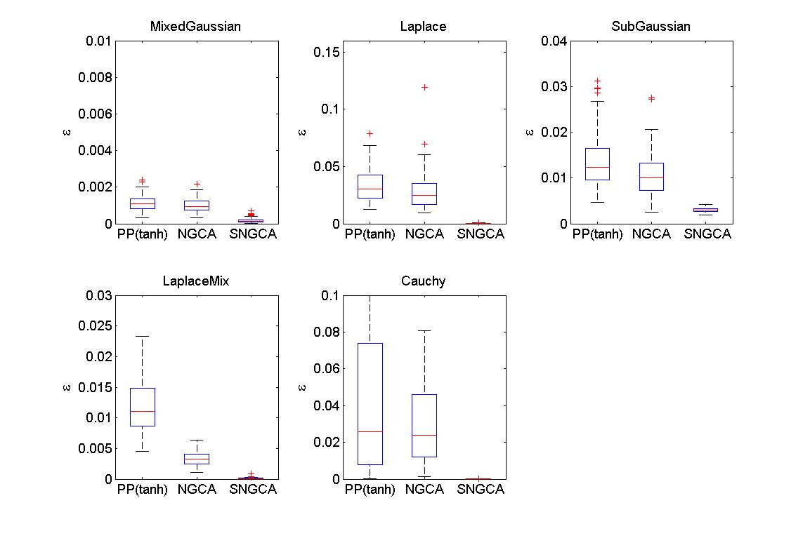
We start with comparing the presented algorithm with Projection Pursuit (PP) method [16] and the NGCA for d=10d=10. The results are presented on Figure 2 (the corresponding results for PP and NGCA has been already reported in [10] and [6]).
Refer to caption
Figure 2: Comparison of PP, NGCA and SNGCA(SDP)

Since the minimization procedure of PP tends to be trapped in a local minimum, in each of the 100 simulations, the PP algorithm is restarted 10 times with random starting points. The best result is reported for each PP-simulation. We observe that SNGCA(SDP) outperforms NGCA and PP in all tests.

In the next simulation we study the dependence of the accuracy of the SNGCA(SDP) on the noise level and compare it to the corresponding data for PP and NGCA. We present on Figure 3 the results of experiments when the non-Gaussian coordinates have unit variance, but the standard deviation of the components of the 88-dimensional Gaussian distribution follows the geometrical progression 10−r,10−r+2​r/7,…,10r10^{-r},10^{-r+2r/7},\ldots,10^{r} where r=1,…,8r=1,\ldots,8.

Refer to caption
Figure 3: estimation error with respect to the standard deviation of Gaussian components following a geometrical progression on [10−r,10r][10^{-r},10^{r}] where rr is the parameter on the abscissa

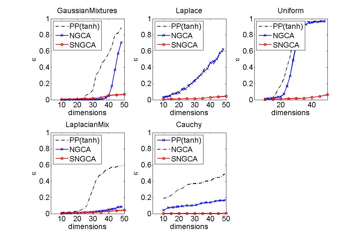
The conditioning of the covariance matrix heavily influences the estimation error of PP(tanh) and NGCA, but not that of SNGCA(SDP). The latter method appears to be insensitive to the differences in the noise variance along different direction in all test cases.

Next we compare the behavior of SNGCA(SDP), PP and NGCA as the dimension of the Gaussian component increases. On Figure 4 we plot the mean error of estimation against the problem dimension dd.

Refer to caption
Figure 4: mean-square estimation error vs problem dimension dd

For PP and NGCA methods we observe that the estimation becomes meaningless (the estimation error explodes) already for d=30−40d=30-40 for the models (A), (C) and for d=20−30d=20-30 of the model (D). In the case of the models (B) and (E) we observe the progressive increase of the error for methods PP and NGCA. The proposed method SNGCA(SDP) behaves robustly with respect to the increasing dimension of the Gaussian component for all test models.

5.3 Application to Geometric Analysis of Metastability

Some biologically active molecules exhibit different large geometric structures at the scale much larger than the diameter of the atoms. If there are more than one such structures with the life span much larger that the time scale of the local atomic vibrations, the structure is called metastable conformation [27]. In other words, metastable conformations of biomolecules can be seen as connected subsets of state-space. When compared to the fluctuations within each conformation, the transitions between different conformations of a molecule are rare statistical events. Such multi-scale dynamic behavior of biomolecules stem from a decomposition of the free energy landscape into particulary deep wells each containing many local minima [23, 12]. Such wells represent different almost invariant geometrical large scale structures [1]. The macroscopic dynamics is assumed to be a Markov jump process, hopping between the metastable sets of the state space while the microscopic dynamics within these sets mixes on much shorter time scales [14]. Since the shape of the energy landscape and the invariant density of the Markov process are unknown, the “essential degrees of freedom”, in which the rare conformational changes occur, are of importance.

We will now illustrate that SNGCA(SDP) is able to detect a multimodal component of the data density as a special case of non-Gaussian subspace in high-dimensional data obtained from molecular dynamics simulation of oligopeptides.

Clustering of 8-alanine

The first example is a times series, generated by an equilibrium molecular dynamics simulation of 8-alanine. We only consider the backbone dihedral angles in order to determine different conformations.

The 1414-dimensional time series consists of the cyclic data set of all backbone torsion angles. The simulation using CHARMM was done at T=300​KT=300K with implicit water by means of the solvent model ACE2 [26]. A symplectic Verlet integrator with integration step of 1​f​s1fs was used; the total trajectory length was 4​μ​s4\mu s and every τ=50​f​s\tau=50fs a set of coordinates was recorded.

The dimension reduction reported in the next figure was obtained using SNGCA(SDP) with for a given dimension m=5m=5 of the target space containing the multimodal component.

Refer to caption
Figure 5: low dimensional multimodal component of 8-alanine

A concentration of the clustered data in the target space of SNGCA may be clearly observed. In comparison, the complement of the target space is almost completely filled with Gaussian noise.

Refer to caption
Figure 6: Gaussian noise in the complement of the SNGCA target space.

Clustering of a 3-peptide molecule

In the next example we investigate Phenylalanyl-Glycyl-Glycine Tripeptide, which is assumed to realize all of the most important folding mechanisms of polypeptides [24]. The simulation is done using GROMACS at T=300​KT=300K with implicit water. An integration step of a symplectic Verlet integrator is set to 2​f​s2fs, and every τ=50​f​s\tau=50fs a set of 31 diedre angles was recorded. As in the previous experience, the dimension of the target space is set to m=5m=5

Figure 7 shows that the clustered data can be primarily found in the target space of SNGCA(SDP).

Refer to caption
Figure 7: low dimensional multimodal component of 3-peptide

6 Conclusions

We have studied a new procedure of non-Gaussian component analysis. The suggested method, same as the techniques proposed in [6, 10], has two stages: on the first stage certain linear functionals of unknown distribution are computed, then this information is used to recover the non-Gaussian subspace. The novelty of the proposed approach resides in the new method of non-Gaussian subspace identification, based upon semidefinite relaxation. The new procedure allows to overcome the main drawbacks of the previous implementations of the NGCA and seems to improve significantly the accuracy of estimation.

On the other hand, the proposed algorithm is computationally demanding. While the first-order optimization algorithm we propose allows to treat efficiently the problems which are far beyond the reach of classical SDP-optimization techniques, the numerical difficulty seems to be the main practical limitation of the proposed approach.

References

  • [1] A. Amadei & A. B. Linssen & H. J. Berendsen (1993) Essential dynamics of proteins. Proteins, 17(4):412-425.
  • [2] A. d’Aspremont, L. El Ghaoui, M.I. Jordan, and G. R. G. Lanckriet (2007) A direct formulation for sparse PCA using semidefinite programming. SIAM Review, 49(3):434-448.
  • [3] A. d’Aspremont, F. Bach and L. El Ghaoui (2008) Optimal solutions for sparse principal component analysis. Journal of Machine Learning Research, 9:1269-1294.
  • [4] M. Belkin, P. Niyogi (2009) Laplacian Eigenmaps for dimensionality reduction and data representation Neural Computation, 15(6):1373-1396.
  • [5] A. Ben Tal & A. Nemirovski (2001) Lectures on Modern Convex Optimization. Analysis, Algorithms and Engineering Applications, Volume 1 of MPS/ SIAM Series on Optimization, SIAM, Philadelphia.
  • [6] G. Blanchard, M. Kawanabe, M. Sugiyama, V. Spokoiny, K.-R. Müller (2006) In Search of Non-Gaussian Components of a High-Dimensional Distribution. J. of Machine Learning Research, p. 247-282.
  • [7] M.Kawanabe, M.Sugiyama, G.Blanchard and K.-R.M’́uller” (2007) A new algorithm of non-Gaussian component analysis with radial kernel functions, Annals of the Institute of Statistical Mathematics, vol. 59(1), 57-75.
  • [8] E. Candès (2006) Compressive sampling. Int. Congress of Mathematics, Madrid, Spain, 3:1433-1452.
  • [9] P. Diaconis & D. Freedman (1984) Asymptotics of graphical projection pursuit Annals of Statistics, 12:793-815.
  • [10] E. Diederichs & A. Juditsky & V. Spokoiny & C. Schütte (2009) Sparse NonGaussian Component Analysis. IEEE Transactions on Information Theory, 15(7):5249-5262.
  • [11] I. Guyon & A. Elisseeff (2003) An Introduction to Variable and Feature Selection. Journal of Machine Learning Research, 3:1157-1182.
  • [12] H. Frauenfelder & B.H. McMahon (2000) Energy Landscape and fluctations in proteins. Ann. Phys. (Leipzig),9:655-667.
  • [13] T. J. Hastie & R. Tibshirani & J. Friedman (2001) The Elements of Statistical Learning. New York, Springer Series in Statistcs.
  • [14] I. Horenko & Ch. Schütte (2008) Likelihood-Based Estimation of Multidimensional Langevin Models and its Application to Biomolecular Dynamics. Mult. Mod. Sim., 7(2):731-773.
  • [15] R. A. Horn and C. R. Johnson (1985) Matrix Analysis. Cambridge University Press.
  • [16] A. Hyvärinen. (1999) Survey on independent component analysis. Neural Computing Surveys, 2:94-128.
  • [17] M. Mizuta (2004) Dimension Reduction Methods. In J.E. Gentle & W. Härdle, and Y. Mori (eds.): Handbook of Computational Statistics pp. 566-89.
  • [18] A. Nemirovski & D. Yudin (1983) Problem Complexity and Method Efficiency in Optimization. New York, J. Wiley and Sons
  • [19] A. Nemirovski (2004) Prox-method with rate of convergence 𝒪⁡(1/t)\mathcal{O}(1/t) for variational inequalities with Lipschitz continuous monotone operators and smooth convex-concave saddle point problems. SIAM Journal on Optimization, 15:229-251
  • [20] Z. Lu & R. Monteiro &A. Nemirovski (2007) Large-Scale Semidefinite Programming via Saddle Point Mirror-Prox Algorithm. Mathematical Programming, 109:2-3, 211-237.
  • [21] Yu. E. Nesterov (2005) Smooth minimization of non-smooth functions. Mathematical Programming: Series A and B, 103(1):127-152.
  • [22] Yu. E. Nesterov (2007) Dual extrapolation and its applications for solving variational inequalities and related problems. Mathematical Programming: Series A and B, 109(2):319-344.
  • [23] J. Pillardy & L. Piela (1995) Molecular dynamics on deformed energy hypersurfaces. J.Phys.Chem., 99:11805-11812.
  • [24] D. Reha & H. Valdes & J.Vondrasek & P. Hobza & A. Abu-Riziq & B. Crews & M.S. de Vries (2005) Structure an IR Spectrum of Phenylalanyl-Glycyl-Glycine Tripeptide in the Gas-Phase. Cem. Eur. J., 11:6083-6817.
  • [25] S. Roweis & L. Saul (2000) Nonlinear dimensionality reduction by locally linear embedding. Science, 290:2323-2326.
  • [26] M. Schaefer & M. Karplus (1996) A Comprehensive Analytical Treatment of Continuum Electrostatics. J. Chem. Phys., 100:1578-1599.
  • [27] C. Schütte & W. Huisinga (2003) Biomolecular Conformations can be identified as metastable sets of melcular dynamics. Computational Chemistry, Handbook of Numerical Analysis, 699-744.
  • [28] V. Spokoiny (2009) A penalized exponential risk bound in parametric estimation. http://arxiv.org/abs/0903.1721.
  • [29] Tenenbaum & V. de Silva & J.C. Langford (2000) A global geometric framework for nonlinear dimensionality reduction. Science, 290:2319-2323.
  • [30] A. van der Vaart & J.A. Wellner (1996) Weak Convergence and Empirical Proccesses. Springer Series in Statistics - New York
  • [31] L. Wasserman (2006) All of Nonparametric Statistics. New York, Springer Texts in Statistcss

Appendix A Appendix

Let X=XT∈ℝL×LX=X^{T}\in\mathbb{R}^{L\times L} be positive semidefinite with |X|1≤1|X|_{1}\leq 1, and let Y=X1/2Y=X^{1/2} be the symmetric positive semidefinite square root of XX. If we denote yi,i=1,..,Ly_{i},\,i=1,..,L the columns of YY, then |X|1≤1|X|_{1}\leq 1 implies that

∑1≤i,j≤L|yiT​yj|≤1.\sum_{1\leq i,j\leq L}|y_{i}^{T}y_{j}|\leq 1.

We make here one trivial though useful observation: for any matrix A∈ℝd×LA\in\mathbb{R}^{d\times L}, when denoting B=AT​AB=A^{T}A, we have

‖A​Y‖22\displaystyle\|AY\|^{2}_{2} =\displaystyle= trace⁡(AT​A​X)=trace⁡[B​X]=∑j=1L∑i=1LBj​i​Xi​j≤maxi​j⁡|Bi​j|=|A|22.\displaystyle\mathrm{trace\,}(A^{T}AX)=\mathrm{trace\,}[BX]=\sum_{j=1}^{L}\sum_{i=1}^{L}B_{ji}X_{ij}\leq\max_{ij}|B_{ij}|=|A|_{2}^{2}. (40)

(Recall that for a matrix A∈ℝd×LA\in\mathbb{R}^{d\times L} with columns aia_{i}, i=1,…,Li=1,...,L, |A|2|A|_{2} stands for the maximal column norm: |A|2=max1≤i≤L⁡|ai|2|A|_{2}=\max_{1\leq i\leq L}|a_{i}|_{2}).

We can rewrite the problem  (3.2) using Y=X1/2Y=X^{1/2}, so that the objective

f^​(X,P)=trace⁡[U^T​(I−P)​U^​X]\displaystyle\widehat{f}(X,P)=\mathrm{trace\,}[\widehat{U}^{T}(I-P)\widehat{U}X]

of  (3.2) becomes

g^​(Y,P)=‖(I−P)1/2​U^​Y‖22.\widehat{g}(Y,P)=\|(I-P)^{1/2}\widehat{U}Y\|_{2}^{2}.

Let now (X^,P^)(\widehat{X},\widehat{P}) be a saddle point of  (3.2). Namely, we have for any feasible PP and XX:

f^(X,P^)≤[f^∗≡f^(X^,P^)]≤f^(X^,P),\widehat{f}(X,\widehat{P})\leq[\widehat{f}_{*}\equiv\widehat{f}(\widehat{X},\widehat{P})]\leq\widehat{f}(\widehat{X},P),

We denote Y^=X^1/2\widehat{Y}=\widehat{X}^{1/2}.

In what follows we suppose that vectors γℓ\gamma_{\ell} and ηℓ\eta_{\ell}, ℓ=1,…,L\ell=1,...,L satisfy  (11). In other words,it holds |U^−U|2≤δN|\widehat{U}-U|_{2}\leq\delta_{N} and |G^−G|2≤γN|\widehat{G}-G|_{2}\leq\gamma_{N}.

A.1 Proof of Theorem 1.

Lemma 1

Let P^\widehat{P} be an optimal solution to  (3.2). Then

maxc{|(I−P^)1/2Uc|2||c|1≤1,Gc=0}≤λmin−1(Σ)(ϱ+νN)+2δN.\displaystyle\max_{c}\left\{|(I-\widehat{P})^{1/2}Uc|_{2}\,\left|\;|c|_{1}\leq 1,\;Gc=0\right.\right\}\leq\lambda_{\min}^{-1}(\Sigma)(\varrho+\nu_{N})+2\delta_{N}. (41)

Proof. We write:

maxc{|(I−P^)1/2Uc|2||c|1≤1,Gc=0}\displaystyle\max_{c}\left\{|(I-\widehat{P})^{1/2}Uc|_{2}\left|\;|c|_{1}\leq 1,\;Gc=0\right.\right\}
≤\displaystyle\leq maxY{∥(I−P^)1/2UY∥2||Y2|1≤1,GY=0}\displaystyle\max_{Y}\left\{\|(I-\widehat{P})^{1/2}UY\|_{2}\left|\;\;|Y^{2}|_{1}\leq 1,\;GY=0\right.\right\}
≤\displaystyle\leq maxY{∥(I−P^)1/2U^Y∥2||Y2|1≤1,GY=0}\displaystyle\max_{Y}\left\{\|(I-\widehat{P})^{1/2}\widehat{U}Y\|_{2}\left|\;\;|Y^{2}|_{1}\leq 1,\;GY=0\right.\right\}
+maxY{∥(I−P^)1/2(U^−U)Y∥2||Y2|1≤1,GY=0}\displaystyle+\max_{Y}\left\{\|(I-\widehat{P})^{1/2}(\widehat{U}-U)Y\|_{2}\left|\;\;|Y^{2}|_{1}\leq 1,\;GY=0\right.\right\}
≤\displaystyle\leq maxY{∥(I−P^)1/2U^Y∥2||Y2|1≤1,∥G^Y∥2≤ϱ}\displaystyle\max_{Y}\left\{\|(I-\widehat{P})^{1/2}\widehat{U}Y\|_{2}\left|\;\;|Y^{2}|_{1}\leq 1,\;\|\widehat{G}Y\|_{2}\leq\varrho\right.\right\}
(by  (40)) +|(I−P^)1/2​(U^−U)|2\displaystyle+|(I-\widehat{P})^{1/2}(\widehat{U}-U)|_{2}
(due to 0⪯I−P^⪯I0\preceq I-\widehat{P}\preceq I) =\displaystyle= ‖(I−P^)1/2​U^​Y^‖2+δN≤‖(I−Π∗)1/2​U^​Y^‖2+δN\displaystyle\|(I-\widehat{P})^{1/2}\widehat{U}\widehat{Y}\|_{2}+\delta_{N}\leq\|(I-\Pi^{*})^{1/2}\widehat{U}\widehat{Y}\|_{2}+\delta_{N}
(again by  (40)) ≤\displaystyle\leq ‖(I−Π∗)1/2​U​Y^‖2+2​δN.\displaystyle\|(I-\Pi^{*})^{1/2}U\widehat{Y}\|_{2}+2\delta_{N}.

On the other hand, as ‖G^​Y^‖2≤νN\|\widehat{G}\widehat{Y}\|_{2}\leq\nu_{N}, we get

‖G​Y^‖2≤‖G^​Y^‖2+‖(G^−G)​Y^‖2≤ϱ+|G^−G|2≤ϱ+νN,\|G\widehat{Y}\|_{2}\leq\|\widehat{G}\widehat{Y}\|_{2}+\|(\widehat{G}-G)\widehat{Y}\|_{2}\leq\varrho+|\widehat{G}-G|_{2}\leq\varrho+\nu_{N},

and by  (3),

‖(I−Π∗)​U​Y^‖2≤λmin−1​(Σ)​(ϱ+νN).\|(I-\Pi^{*})U\widehat{Y}\|_{2}\leq\lambda_{\min}^{-1}(\Sigma)(\varrho+\nu_{N}).

This implies  (41). □\,\Box\quad\,
We now come back to the proof of the theorem. Let λ^j\widehat{\lambda}_{j} and θ^j\widehat{\theta}_{j}, j=1,…,dj=1,\ldots,d be respectively the eigenvalues and the eigenvectors of P^\widehat{P}. Assume that λ^1≥λ^2≥…≥λ^d\widehat{\lambda}_{1}\geq\widehat{\lambda}_{2}\geq\ldots\geq\widehat{\lambda}_{d}. Then P^=∑j=1dλ^j​θ^j​θ^jT\widehat{P}=\sum_{j=1}^{d}\widehat{\lambda}_{j}\widehat{\theta}_{j}\widehat{\theta}_{j}^{T} and Π^=∑j=1mθ^j​θ^jT\widehat{\Pi}=\sum_{j=1}^{m}\widehat{\theta}_{j}\widehat{\theta}_{j}^{T}. Let β=U​c\beta=Uc for cc such that |c|1≤1|c|_{1}\leq 1 and G​c=0Gc=0. We have

βT​(I−P^)​β\displaystyle\beta^{T}(I-\widehat{P})\beta =\displaystyle= ∑j=1m(1−λ^j)​(θ^jT​β)2+∑j>m(1−λ^j)​(θ^jT​β)2\displaystyle\sum_{j=1}^{m}(1-\widehat{\lambda}_{j})(\widehat{\theta}_{j}^{T}\beta)^{2}+\sum_{j>m}(1-\widehat{\lambda}_{j})(\widehat{\theta}_{j}^{T}\beta)^{2}
≥\displaystyle\geq ∑j>m(1−λ^j)​(θ^jT​β)2≥(1−λ^m+1)​(θ^jT​β)2\displaystyle\sum_{j>m}(1-\widehat{\lambda}_{j})(\widehat{\theta}_{j}^{T}\beta)^{2}\geq(1-\widehat{\lambda}_{m+1})(\widehat{\theta}_{j}^{T}\beta)^{2}
=\displaystyle= (1−λ^m+1)​βT​(I−Π^)​β=(1−λ^m+1)​|(I−Π^)​β|22.\displaystyle(1-\widehat{\lambda}_{m+1})\beta^{T}(I-\widehat{\Pi})\beta=(1-\widehat{\lambda}_{m+1})|(I-\widehat{\Pi})\beta|^{2}_{2}.

Since, for obvious reasons, λ^m+1≤mm+1\widehat{\lambda}_{m+1}\leq{m\over m+1}, it applies (i) due to  (41).

Let us show (ii). We have due to  (23) and  (41):

trace⁡[(I−P^)​Π∗]=trace⁡[(I−P^)1/2​Π∗​(I−P^)1/2]\displaystyle\mathrm{trace\,}\left[(I-\widehat{P})\Pi^{*}\right]=\mathrm{trace\,}\left[(I-\widehat{P})^{1/2}\Pi^{*}(I-\widehat{P})^{1/2}\right] (42)
≤\displaystyle\leq ∑k=1mμk​trace​[(I−P^)1/2​U​ck​ckT​UT​(I−P^)1/2]=∑k=1mμk​|(I−P^)1/2​U​ck|22\displaystyle\sum_{k=1}^{{m}}\mu_{k}\mathrm{trace\,}\left[(I-\widehat{P})^{1/2}Uc_{k}c_{k}^{T}U^{T}(I-\widehat{P})^{1/2}\right]=\sum_{k=1}^{{m}}\mu_{k}|(I-\widehat{P})^{1/2}Uc_{k}|_{2}^{2}
≤\displaystyle\leq ∑k=1mμkmaxc{|(I−P^)1/2Uc|22||c|1≤1,Gc=0}\displaystyle\sum_{k=1}^{{m}}\mu_{k}\max_{c}\left\{|(I-\widehat{P})^{1/2}Uc|_{2}^{2}\left|\;|c|_{1}\leq 1,\;Gc=0\right.\right\}
=\displaystyle= μ∗​(λmin−1​(Σ)​(ϱ+νN)+2​δN)2,\displaystyle\mu^{*}(\lambda_{\min}^{-1}(\Sigma)(\varrho+\nu_{N})+2\delta_{N})^{2},

which is  (24).

Note that trace⁡[P^​Π∗]≤∑j≤mλ^j\mathrm{trace\,}[\widehat{P}\Pi^{*}]\leq\sum_{j\leq m}\widehat{\lambda}_{j} (cf, e.g., Corollary 4.3.18 of [15]), thus by  (42),

λ^m+1≤m−∑j≤mλ^j≤trace⁡[(I−P^)​Π∗]≤μ∗​(λmin−1​(Σ)​(ϱ+νN)+2​δN)2.\widehat{\lambda}_{m+1}\leq m-\sum_{j\leq m}\widehat{\lambda}_{j}\leq\mathrm{trace\,}[(I-\widehat{P})\Pi^{*}]\leq\mu^{*}(\lambda_{\min}^{-1}(\Sigma)(\varrho+\nu_{N})+2\delta_{N})^{2}.

On the other hand,

trace⁡[(I−P^)​Π∗]\displaystyle\mathrm{trace\,}[(I-\widehat{P})\Pi^{*}] =\displaystyle= ∑j=1m(1−λ^j)​θ^jT​Π∗​θ^j+∑j>m(1−λ^j)​θ^jT​Π∗​θ^j\displaystyle\sum_{j=1}^{m}(1-\widehat{\lambda}_{j})\widehat{\theta}_{j}^{T}\Pi^{*}\widehat{\theta}_{j}+\sum_{j>m}(1-\widehat{\lambda}_{j})\widehat{\theta}_{j}^{T}\Pi^{*}\widehat{\theta}_{j}
≥\displaystyle\geq ∑j>m(1−λ^j)​θ^jT​Π∗​θ^j≥(1−λ^m+1)​θ^jT​Π∗​θ^j\displaystyle\sum_{j>m}(1-\widehat{\lambda}_{j})\widehat{\theta}_{j}^{T}\Pi^{*}\widehat{\theta}_{j}\geq(1-\widehat{\lambda}_{m+1})\widehat{\theta}_{j}^{T}\Pi^{*}\widehat{\theta}_{j}
=\displaystyle= (1−λ^m+1)​trace​[(I−Π^)​Π∗],\displaystyle(1-\widehat{\lambda}_{m+1})\mathrm{trace\,}[(I-\widehat{\Pi})\Pi^{*}],

and we conclude that

trace⁡[(I−Π^)​Π∗]≤trace⁡[(1−P^)​Π∗]1−λ^m+1≤μ∗​(λmin−1​(Σ)​(ϱ+νN)+2​δN)21−μ∗​(λmin−1​(Σ)​(ϱ+νN)+2​δN)2.\mathrm{trace\,}[(I-\widehat{\Pi})\Pi^{*}]\leq{\mathrm{trace\,}[(1-\widehat{P})\Pi^{*}]\over 1-\widehat{\lambda}_{m+1}}\leq{\mu^{*}(\lambda_{\min}^{-1}(\Sigma)(\varrho+\nu_{N})+2\delta_{N})^{2}\over 1-\mu^{*}(\lambda_{\min}^{-1}(\Sigma)(\varrho+\nu_{N})+2\delta_{N})^{2}}.

Now, using the relation trace​Π^=trace​Π∗=m\mathrm{trace\,}\widehat{\Pi}=\mathrm{trace\,}\Pi^{*}=m, we come to

‖Π^−Π∗‖22=trace⁡[Π^2−2​Π^​Π∗+(Π∗)2]=2​m−2​trace​[Π^​Π∗]=2​trace​[(I−Π^)​Π∗],\|\widehat{\Pi}-\Pi^{*}\|_{2}^{2}=\mathrm{trace\,}[\widehat{\Pi}^{2}-2\widehat{\Pi}\Pi^{*}+(\Pi^{*})^{2}]=2m-2\mathrm{trace\,}[\widehat{\Pi}\Pi^{*}]=2\mathrm{trace\,}[(I-\widehat{\Pi})\Pi^{*}],

and we arrive at  (1).

A.2 Proof of Theorem 2.

Let now P^,X^\widehat{P},\;\widehat{X} and t^=trace​P^\widehat{t}=\mathrm{trace\,}\widehat{P} be a triplet of optimal solution to  (3.3).

Lemma 2

Let P^\widehat{P} be an optimal solution to  (3.3).

In the premises of the theorem Π∗\Pi^{*} is a feasible solution of  (3.3) and trace​P^≤trace​Π∗=m\mathrm{trace\,}\widehat{P}\leq\mathrm{trace\,}\Pi^{*}=m.

We have

maxc{|(I−P^)1/2Uc|2||c|1≤1,Gc=0}≤ρ+δN.\displaystyle\max_{c}\left\{|(I-\widehat{P})^{1/2}Uc|_{2}\,\left|\;|c|_{1}\leq 1,\;Gc=0\right.\right\}\leq\rho+\delta_{N}. (43)

Proof. We act as in the proof of Lemma 1: to verify (i)(i) we observe that

maxX{trace[U^T(I−Π∗)U^X]|X⪰0,|X|1≤1,trace[G^XG^T]≤ϱ2}\displaystyle\max_{X}\left\{\mathrm{trace\,}[\widehat{U}^{T}(I-\Pi^{*})\widehat{U}X]\left|\;X\succeq 0,\;|X|_{1}\leq 1,\;\mathrm{trace\,}[\widehat{G}X\widehat{G}^{T}]\leq\varrho^{2}\right.\right\}
=\displaystyle= maxY{∥(I−Π∗)U^Y∥22||Y2|1≤1,∥G^Y∥2≤ϱ}\displaystyle\max_{Y}\left\{\|(I-\Pi^{*})\widehat{U}Y\|^{2}_{2}\left|\;\;|Y^{2}|_{1}\leq 1,\;\|\widehat{G}Y\|_{2}\leq\varrho\right.\right\}
≤\displaystyle\leq maxY{(∥(I−Π∗)UY∥2+δN)2||Y2|1≤1,∥G^Y∥2≤ϱ}\displaystyle\max_{Y}\left\{(\|(I-\Pi^{*})UY\|_{2}+\delta_{N})^{2}\left|\;\;|Y^{2}|_{1}\leq 1,\;\|\widehat{G}Y\|_{2}\leq\varrho\right.\right\}
≤\displaystyle\leq (λm​i​n−1​(Σ)​(ϱ+νN)+δN)2.\displaystyle\left(\lambda^{-1}_{min}(\Sigma)(\varrho+\nu_{N})+\delta_{N}\right)^{2}.

Thus, if ρ≥λm​i​n−1​(Σ)​(ϱ+νN)+δN\rho\geq\lambda^{-1}_{min}(\Sigma)(\varrho+\nu_{N})+\delta_{N}, Π∗\Pi^{*} is a feasible solution of  (3.3) and, as a result, trace​P^≤trace​Π∗\mathrm{trace\,}\widehat{P}\leq\mathrm{trace\,}\Pi^{*}. To show (i​i)(ii) it suffices to note that

maxc{|(I−P^)1/2Uc|2||c|1≤1,Gc=0}\displaystyle\max_{c}\left\{|(I-\widehat{P})^{1/2}Uc|_{2}\left|\;|c|_{1}\leq 1,\;Gc=0\right.\right\}
≤\displaystyle\leq maxY{∥(I−P^)1/2UY∥2||Y2|1≤1,GY=0}\displaystyle\max_{Y}\left\{\|(I-\widehat{P})^{1/2}UY\|_{2}\left|\;\;|Y^{2}|_{1}\leq 1,\;GY=0\right.\right\}
≤\displaystyle\leq maxY{∥(I−P^)1/2U^Y∥2||Y2|1≤1,GY=0}+|(I−P^)1/2(U^−U)|2\displaystyle\max_{Y}\left\{\|(I-\widehat{P})^{1/2}\widehat{U}Y\|_{2}\left|\;\;|Y^{2}|_{1}\leq 1,\;GY=0\right.\right\}+|(I-\widehat{P})^{1/2}(\widehat{U}-U)|_{2}
≤\displaystyle\leq maxY{∥(I−P^)1/2U^Y∥2||Y2|1≤1,∥G^Y∥2≤ϱ}+δN≤ρ+δN\displaystyle\max_{Y}\left\{\|(I-\widehat{P})^{1/2}\widehat{U}Y\|_{2}\left|\;\;|Y^{2}|_{1}\leq 1,\;\|\widehat{G}Y\|_{2}\leq\varrho\right.\right\}+\delta_{N}\leq\rho+\delta_{N}

because of the feasibility of P^\widehat{P}. □\,\Box\quad\,
Now using the bound m^≤m\widehat{m}\leq m we complete the proof following exactly the lines of the proof of Theorem 1.

A.3 Proof of Proposition 1

Observe that

F¯​(Z^,Y^)\displaystyle\underline{F}(\widehat{Z},\widehat{Y}) =\displaystyle= min(P,W)∈𝒫×𝒲⁡{trace⁡[BT​(I−P)​B​QT​Z^​Q]+λ​trace​[W⁡(QT​Z^​Q−Y^)]}\displaystyle\min_{(P,W)\in\mathcal{P}\times\mathcal{W}}\left\{\mathrm{trace\,}[B^{T}(I-P)BQ^{T}\widehat{Z}Q]+\lambda\,\mathrm{trace\,}[W(Q^{T}\widehat{Z}Q-\widehat{Y})]\right\} (44)
=\displaystyle= minP∈𝒫⁡{trace⁡[BT​(I−P)​B​QT​Z^​Q]−λ​‖QT​Z^​Q−Y^‖2}\displaystyle\min_{P\in\mathcal{P}}\left\{\mathrm{trace\,}[B^{T}(I-P)BQ^{T}\widehat{Z}Q]-\lambda\,\|Q^{T}\widehat{Z}Q-\widehat{Y}\|_{2}\right\}
≤\displaystyle\leq minP∈𝒫⁡{trace⁡[BT​(I−P)​B​QT​Z^​Q]}=G¯​(Z^);\displaystyle\min_{P\in\mathcal{P}}\left\{\mathrm{trace\,}[B^{T}(I-P)BQ^{T}\widehat{Z}Q]\right\}=\underline{G}(\widehat{Z});

and

F¯​(P^,W^)\displaystyle\overline{F}(\widehat{P},\widehat{W}) =\displaystyle= max(Z,Y)∈𝒵×𝒴⁡{trace⁡[BT​(I−P^)​B​QT​Z​Q]+λ​trace​[W^​(QT​Z​Q−Y)]}\displaystyle\max_{(Z,Y)\in\mathcal{Z}\times\mathcal{Y}}\left\{\mathrm{trace\,}[B^{T}(I-\widehat{P})BQ^{T}ZQ]+\lambda\,\mathrm{trace\,}[\widehat{W}(Q^{T}ZQ-Y)]\right\}
≥\displaystyle\geq maxZ∈𝒵,|QT​Z​Q|1≤1,Y=QT​Z​Q⁡{trace⁡[BT​(I−P^)​B​QT​Z​Q]+λ​trace​[W^​(QT​Z​Q−Y)]}\displaystyle\max_{Z\in\mathcal{Z},\;|Q^{T}ZQ|_{1}\leq 1,\,Y=Q^{T}ZQ}\left\{\mathrm{trace\,}[B^{T}(I-\widehat{P})BQ^{T}ZQ]+\lambda\,\mathrm{trace\,}[\widehat{W}(Q^{T}ZQ-Y)]\right\}
=\displaystyle= G¯​(P^):\displaystyle\overline{G}(\widehat{P}):

Assume first that |QT​Z^​Q|1≤1|Q^{T}\widehat{Z}Q|_{1}\leq 1. In this case Z~=Z^\widetilde{Z}=\widehat{Z} and

ϵ≥F¯​(P^,W^)−F¯​(Z^,Y^)=G¯​(P^)−G¯​(Z^)=G¯​(P^)−G¯​(Z~)\epsilon\geq\overline{F}(\widehat{P},\widehat{W})-\underline{F}(\widehat{Z},\widehat{Y})=\overline{G}(\widehat{P})-\underline{G}(\widehat{Z})=\overline{G}(\widehat{P})-\underline{G}(\widetilde{Z})

(the second ¸ is given by  (44)), as claimed. Now assume that s=QT​Z^​Q|1>1s=Q^{T}\widehat{Z}Q|_{1}>1. We have already established the first equality of the following chain:

F¯​(Z^,Y^)=minP∈𝒫⁡{trace⁡(BT​(I−P)​B​QT​Z^​Q)−λ​‖QT​Z^​Q−Y^‖2}\displaystyle\underline{F}(\widehat{Z},\widehat{Y})=\min_{P\in\mathcal{P}}\left\{\mathrm{trace\,}(B^{T}(I-P)BQ^{T}\widehat{Z}Q)-\lambda\,\|Q^{T}\widehat{Z}Q-\widehat{Y}\|_{2}\right\}
≤\displaystyle\leq minP∈𝒫⁡{trace⁡[BT​(I−P)​B​QT​Z^​Q]−λL|QT​Z^​Q−Y^|1}\displaystyle\min_{P\in\mathcal{P}}\left\{\mathrm{trace\,}[B^{T}(I-P)BQ^{T}\widehat{Z}Q]-{\lambda\over L}|Q^{T}\widehat{Z}Q-\widehat{Y}|_{1}\right\}
≤\displaystyle\leq minP∈𝒫⁡{trace⁡[BT​(I−P)​B​QT​Z^​Q]−λL​(s−1)}\displaystyle\min_{P\in\mathcal{P}}\left\{\mathrm{trace\,}[B^{T}(I-P)BQ^{T}\widehat{Z}Q]-{\lambda\over L}(s-1)\right\}
=\displaystyle= minP∈𝒫⁡{s​trace​[BT​(I−P)​B​QT​Z~​Q]−λL​(s−1)}\displaystyle\min_{P\in\mathcal{P}}\left\{s\mathrm{trace\,}[B^{T}(I-P)BQ^{T}\widetilde{Z}Q]-{\lambda\over L}(s-1)\right\}
≤\displaystyle\leq minP∈𝒫⁡{trace⁡[BT​(I−P)​B​QT​Z~​Q]+(s−1)​|BT​(I−P)​B|∞|​QT​Z~​Q|1⏟≤(s−1)​|BT​B|∞=(s−1)​|B|22−λL​(s−1)}\displaystyle\min_{P\in\mathcal{P}}\left\{\mathrm{trace\,}[B^{T}(I-P)BQ^{T}\widetilde{Z}Q]+\underbrace{(s-1)|B^{T}(I-P)B|_{\infty}|Q^{T}\widetilde{Z}Q|_{1}}_{\leq(s-1)|B^{T}B|_{\infty}=(s-1)|B|_{2}^{2}}-{\lambda\over L}(s-1)\right\}
≤\displaystyle\leq minP∈𝒫⁡{trace⁡[BT​(I−P)​B​QT​Z~​Q]}=G¯​(Z~),\displaystyle\min_{P\in\mathcal{P}}\left\{\mathrm{trace\,}[B^{T}(I-P)BQ^{T}\widetilde{Z}Q]\right\}=\underline{G}(\widetilde{Z}),

where the concluding ≤\leq is readily given by the definition of λ\lambda.33 3 We denote |A|∞=maxi​j⁡|Ai​j||A|_{\infty}=\max_{ij}|A_{ij}|. Further, we have already seen that

F¯​(P^,W^)≥G¯​(P^).\overline{F}(\widehat{P},\widehat{W})\geq\overline{G}(\widehat{P}).

Consequently,

ϵ≥F¯​(P^,W^)−F¯​(Z^,Y^)≥G¯​(P^)−G¯​(Z~),\epsilon\geq\overline{F}(\widehat{P},\widehat{W})-\underline{F}(\widehat{Z},\widehat{Y})\geq\overline{G}(\widehat{P})-\underline{G}(\widetilde{Z}),

as claimed. □\,\Box\quad\,

A.4 Computing the prox-transform

Recall that because of the additivity of the distance-generating function dd the computation of the prox-transform on the set 𝒫×𝒲×𝒵×𝒴\mathcal{P}\times\mathcal{W}\times\mathcal{Z}\times\mathcal{Y} can be decomposed into independent computations on the four domains of  (38).

Prox-transform on 𝒫\mathcal{P}.

The proxy-function of 𝒫\mathcal{P} is the matrix entropy:

d⁡(P0,P)=βP​trace​[Pm​(ln⁡(Pm)−ln⁡(P0m))]​for​P,P0∈𝒫,βP>0.\displaystyle d(P_{0},P)=\beta_{P}\mathrm{trace\,}\left[{P\over m}\left(\ln\left({P\over m}\right)-\ln\left({P_{0}\over m}\right)\right)\right]\;\;\mbox{for}\;\;P,P_{0}\in\mathcal{P},\;\;\beta_{P}>0.

To compute the corresponding component of TT we need to find, given S∈𝕊dS\in{\mathbb{S}}^{d},

Tβ​(P0,S)\displaystyle T_{\beta}(P_{0},S) =\displaystyle= arg⁡maxP∈𝒫​{trace⁡[S⁡(P−P0)]−βP​trace​[Pm​(ln⁡(Pm)−ln⁡(P0m))]}\displaystyle\arg\max_{P\in\cal P}\left\{\mathrm{trace\,}[S(P-P_{0})]-\beta_{P}\,\mathrm{trace\,}\left[{P\over m}\left(\ln\left({P\over m}\right)-\ln\left({P_{0}\over m}\right)\right)\right]\right\} (45)
=\displaystyle= arg⁡maxP∈𝒫​{trace⁡[(S+βPm​ln⁡(P0m))​P]−βP​trace​[Pm​ln⁡(Pm)]}.\displaystyle\arg\max_{P\in\cal P}\left\{\mathrm{trace\,}\left[\left(S+{\beta_{P}\over m}\ln\left({P_{0}\over m}\right)\right)P\right]-\beta_{P}\,\mathrm{trace\,}\left[{P\over m}\ln\left({P\over m}\right)\right]\right\}.

By the symmetry considerations we conclude that the optimal solution of this problem is diagonal in the basis of eigenvectors of S+βPm​ln⁡(P0m)S+{\beta_{P}\over m}\ln({P_{0}\over m}). Thus the solution of  (45) can be obtained as follows: compute the eigenvalue decomposition

S+βPm​ln⁡(P0m)=Γ​Λ​ΓT\displaystyle S+{\beta_{P}\over m}\ln({P_{0}\over m})=\Gamma\Lambda\Gamma^{T}

and let λ\lambda be the diagonal of Λ\Lambda. Then solve the “vector” problem

p∗=arg⁡max0≤p≤1,∑p≤m​λT​p−βPm​∑i=1dpi​ln⁡(pi/m).\displaystyle p^{*}=\arg\max_{0\leq p\leq 1,\;\sum p\leq m}\lambda^{T}p-{\beta_{P}\over m}\sum_{i=1}^{d}p_{i}\ln(p_{i}/m). (46)

and compose

Tβ​(P,S)=Γ​diag​(y∗)​ΓT.T_{\beta}(P,S)=\Gamma{\rm diag}(y^{*})\Gamma^{T}.

Now, the solution of  (46) can be obtained by simple bisection: indeed, using Lagrange duality we conclude that the components of y∗y^{*} satisfies

pi∗=exp(λiβ−ν)∧1,i=1,…,d,p^{*}_{i}=\exp\left({\lambda_{i}\over\beta}-\nu\right)\wedge 1,\;\;i=1,...,d,

and the Lagrange multiplier ν\nu is to be set to obtain ∑pi∗=m\sum p^{*}_{i}=m, what can be done by bisection in ν\nu. When the solution is obtained, the optimal value of  (45) can be easily computed.

Prox-transform on 𝒲\mathcal{W}.

The distance-generating function of 𝒲\mathcal{W} is βW​trace​[W2]/2=‖W‖22/2\beta_{W}\mathrm{trace\,}[W^{2}]/2=\|W\|_{2}^{2}/2 so that we have to solve for S∈𝕊LS\in{\mathbb{S}}^{L}

Tβ​(W0,S)\displaystyle T_{\beta}(W_{0},S) =\displaystyle= arg⁡max‖W‖2≤1​{trace⁡[S⁡(W−W0)]−βW2​‖W−W0‖222}.\displaystyle\arg\max_{\|W\|_{2}\leq 1}\left\{\mathrm{trace\,}[S(W-W_{0})]-{\beta_{W}\over 2}{\|W-W_{0}\|_{2}^{2}\over 2}\right\}. (47)

The optimal solution to  (47) can be easily computed

Tβ​(W0,S)={W0+S/βWif‖W0+S/βW‖2≤1,(W0+S/βW)/‖W0+S/βW‖2if‖W0+S/βW‖2>1.T_{\beta}(W_{0},S)=\left\{\begin{array}[]{lcl}W_{0}+S/\beta_{W}&\mbox{if}&\|W_{0}+S/\beta_{W}\|_{2}\leq 1,\\ (W_{0}+S/\beta_{W})/\|W_{0}+S/\beta_{W}\|_{2}&\mbox{if}&\|W_{0}+S/\beta_{W}\|_{2}>1.\end{array}\right.

Prox-transform on 𝒵\mathcal{Z}.

The prox-function of 𝒵\mathcal{Z} is the matrix entropy and we have to solve for S∈𝕊L−dS\in{\mathbb{S}}^{L-d}

Tβ​(Z,S)\displaystyle T_{\beta}(Z,S) =\displaystyle= arg⁡maxZ∈𝒵⁡trace⁡[S⁡(Z−Z0)]−βZ​trace​[Z⁡(ln⁡(Z)−ln⁡(Z0))]\displaystyle\arg\max_{Z\in\cal Z}\mathrm{trace\,}[S(Z-Z_{0})]-\beta_{Z}\mathrm{trace\,}[Z(\ln(Z)-\ln(Z_{0}))]
=\displaystyle= arg⁡maxZ∈𝒵⁡trace⁡[(S+βZ​ln⁡(Z0))​Z]−βZ​trace​[Z​ln​Z].\displaystyle\arg\max_{Z\in\cal Z}\mathrm{trace\,}[(S+\beta_{Z}\ln(Z_{0}))Z]-\beta_{Z}\mathrm{trace\,}[Z\ln Z].

Once again, in the basis of eigenvectors of S+βZ​ln⁡(Z0)S+\beta_{Z}\ln(Z_{0}) the problem reduces to

z∗=arg⁡maxz≥0,∑z≤1​λT​z−βZ​∑i=1dzi​ln⁡(zi),\displaystyle z^{*}=\arg\max_{z\geq 0,\;\sum z\leq 1}\lambda^{T}z-{\beta_{Z}}\sum_{i=1}^{d}z_{i}\ln(z_{i}),

where λ\lambda is the diagonal of Λ\Lambda with S+βZ​ln⁡Z0=Γ​Λ​ΓTS+\beta_{Z}\ln Z_{0}=\Gamma\Lambda\Gamma^{T}. In this case

z∗i=exp⁡(λiβ)∑j=1L¯exp⁡(λjβ),i=1,…,L−d.z^{*}_{i}=\frac{\exp({\lambda_{i}\over\beta})}{\sum_{j=1}^{\overline{L}}\exp({\lambda_{j}\over\beta})},\;\;i=1,...,L-d.

Prox-transform on 𝒴\mathcal{Y}.

The distance generating function for the domain 𝒴\mathcal{Y} is defined as follows:

d⁡(Y)\displaystyle d(Y) =\displaystyle= min{∑i,j=1L(ui​jln[ui​j]+vi​jln[vi​j]):∑i=1n(ui​j+vi​j)=1,\displaystyle\min\left\{\;\sum\limits_{i,j=1}^{L}\left(u_{ij}\ln[u_{ij}]+v_{ij}\ln[v_{ij}]\,\right):\;\sum\limits_{i=1}^{n}(u_{ij}+v_{ij})=1,\right.
Yi​j\displaystyle Y_{ij} =\displaystyle= ui​j−vi​j,ui​j≥0,vi​j≥0, 1≤i,j≤L}.\displaystyle\left.u_{ij}-v_{ij},\;u_{ij}\geq 0,\;v_{ij}\geq 0,\;1\leq i,j\leq L\;\right\}.

In other words, the element Y∈𝒴Y\in\mathcal{Y} is decomposed according to Y=u−vY=u-v, where (u,v)(u,v) is an element of the 2​L22L^{2}-dimensional simplex Δ={x∈ℝ2​L2,x≥0,∑ixi=1}\Delta=\left\{x\in\mathbb{R}^{2L^{2}},\,x\geq 0,\,\sum_{i}x_{i}=1\right\}. To find the YY-component of the prox-transform amounts to find for S∈𝕊LS\in{\mathbb{S}}^{L}

TβY​(Y0,S)\displaystyle T_{\beta_{Y}}(Y_{0},S) =\displaystyle= TβY​(u0,v0,S)\displaystyle T_{\beta_{Y}}(u^{0},v^{0},S) (48)
=\displaystyle= arg⁡maxu,v∈Δ⁡trace⁡[S⁡(u−v)]−βY​∑i​j[ui​j​ln⁡(ui​jui​j0)+vi​j​ln⁡(vi​jvi​j0)].\displaystyle\arg\max_{u,v\in\Delta}\mathrm{trace\,}[S(u-v)]-\beta_{Y}\sum_{ij}\left[u_{ij}\ln({u_{ij}\over u^{0}_{ij}})+v_{ij}\ln({v_{ij}\over v^{0}_{ij}})\right].

One can easily obtain an explicit solution to  (48): let

ai​j=ui​j0​exp⁡(Si​jβY),bi​j=vi​j0​exp⁡(−Si​jβY).\displaystyle a_{ij}=u^{0}_{ij}\exp\left({S_{ij}\over\beta_{Y}}\right),\;\;\;b_{ij}=v^{0}_{ij}\exp\left(-{S_{ij}\over\beta_{Y}}\right).

Then TβY​(Y0,S)=u∗−v∗T_{\beta_{Y}}(Y_{0},S)=u^{*}-v^{*}, where

ui​j∗=ai​j∑i​j(ai​j+bi​j),vi​j∗=bi​j∑i​j(ai​j+bi​j).u^{*}_{ij}={a_{ij}\over\sum_{ij}(a_{ij}+b_{ij})},\;\;v^{*}_{ij}={b_{ij}\over\sum_{ij}(a_{ij}+b_{ij})}.