Rabi-vibronic resonance with large number of vibrational quanta
Abstract
We study theoretically the Rabi oscillations of a resonantly driven two-level system linearly coupled to a harmonic oscillator (vibrational mode) with frequency, . We show that for weak coupling, , where is the polaronic shift, Rabi oscillations are strongly modified in the vicinity of the Rabi-vibronic resonance , where is the Rabi frequency. The width of the resonance is . Within this domain of the actual frequency of the Rabi oscillations exhibits a bistable behavior as a function of . Importantly, within the resonant domain, the oscillator is highly excited, which allows to treat it classically.
pacs
42.65.Pc, 42.50.Md, 78.47.D-, 85.85.+jI Introduction
Coupling to environment tends to damp the Rabi oscillations[1] of a resonantly driven two-level system. Usually, the environment is viewed as medium with continuous spectrum of modes. Less common is the situation when environment possesses a single or several well-defined frequencies. For concreteness we will consider the situation depicted in Fig. 1 when the lower level of the two-level system is coupled to an oscillator (a mass, , and a spring), which represents a single vibrational mode. Obviously, coupling to the oscillator has a strong effect on the Rabi oscillations in the regime of the vacuum Rabi splitting[2] when the oscillator frequency, , is close to the transition frequency, . It is less obvious what effect the coupling to the oscillator will have on the Rabi oscillations when is much smaller than and is comparable to the Rabi frequency, . One can argue on physical grounds that the effect of coupling on the Rabi oscillations will be strong in the vicinity of the condition, , which we dub Rabi-vibronic resonance. Indeed, consider the Hamiltonian
| (1) |
describing the linear coupling. Here is the operator of the oscillator displacement, is a creation operator of the vibrational quantum, is the occupation of the level , and , where is a dimensionless coupling constant. In the course of the Rabi oscillations the average changes with time as

| (2) |
Then at , the second term in Eq. (2) gives rise to a resonant driving force acting on the oscillator. In turn, the strongly driven oscillator provides a resonant feedback [3, 4] on the two-level system. Thus, as , which is proportional to the ac field driving the two-level system, increases, we expect the Rabi oscillations to be strongly modified near the resonant condition.
Among possible experimental realizations of the situation Fig. 1 is a suspended carbon nanotube in inhomogeneous electric field, which creates a confinement for an exciton[5, 6, 7, 8]. Localized exciton can be viewed as a two-level system. Bending modes having discrete frequencies due to finite nanotube length, can be viewed as oscillators with very low friction. While a typical transition frequency in such a system is[10, 9] Hz, the oscillator frequency[7] is much smaller Hz. Resonant condition can be achieved by adjusting the illumination intensity.
Another area in which the situation Fig. 1 is relevant, is the cavity QED[11], where a two-level system is realized in the form of a superconducting qubit, while the oscillator is a LC-circuit. Majority of experimental and theoretical studies in this field are focused on the strong coupling in the domain . However, in experiments Refs. [12, 13] an ac driven superconducting qubit was coupled to a ”slow” LC-oscillator tuned to . It was observed that the noise spectrum of the oscillator exhibits a Lorentzian peak[14] as a function of . In theoretical papers[15, 16, 17] initiated by the experiment Ref. 12 collective motion of the oscillator coupled to a qubit was studied within the density matrix formalism, and both subsystems were treated quantum-mechanically. In view of complexity of this description, final results were obtained numerically for particular values of a coupling parameter, . A notable finding of Refs. [15, 16, 17] is that, in the vicinity of the condition , collective Rabi-vibronic motion becomes bistable.
There are still several basic questions to be answered, among which:
(i) how the frequency, , of the collective oscillations depends on ?
(ii) what is the width of the resonance, i.e., the domain of the Rabi frequencies where Rabi oscillations are modified due to coupling?
(iii) how the decay of the Rabi oscillations depends on the oscillator friction?
The above questions are studied in the present paper. Our main finding is that the width of the Rabi-vibronic resonance is small for weak coupling, namely,
| (3) |
where is the polaronic shift. Eq. (3) suggests that, while is much smaller than , it is much bigger than . Most importantly, Eq. (3) guarantees that, in the resonant domain , the oscillator is highly excited and can be treated as classical. This allows the analytical description of the resonance. In this regard, the situation we consider, two-level system coupled to a classical oscillator, is similar to the Rabi resonance considered in Refs. [18, 19], where two-level system was driven by two classical fields: one with frequency close to and one with frequency close to .
We will see that in the domain , the frequency of collective oscillations differs from also by . Bistable behavior of the dependence emerges naturally within our approach; the frequency jumps between two stable regimes are also . In addition, in the present paper we study how the Rabi-vibronic resonance depends on detuning, , of the driving frequency from , on intrinsic anharmonicity of the oscillator, and how the modified Rabi oscillations decay with time due to relaxation of the two-level system and due to friction in the oscillator.
II Basic equations
We first assume that the displacement, , is a classical variable and will later check this assumption. The equation of motion for reads
| (4) |
where is the population inversion, and is the friction in the oscillator. The equation for and nondiagonal elements of the density matrix have the form of the optical Bloch equations
| (5) |
| (6) |
| (7) |
where is the relaxation rate of the excited state. Note that, while the oscillator is driven by , it exercises a feedback on the two-level system via and .
We require that the level at is occupied while the level is empty, i.e., . We also assume that the dipole moment and dipole current are initially zero, leading to and , respectively. From Eq. (5), we see that the initial conditions for and require that .
III Modified Rabi oscillations
III.1 Oscillation frequency
The system Eqs. (5)-(7) can be reduced to two coupled equations by excluding and expressing in terms of . Then one gets
| (8) |
| (9) |
We start from the simplest case, , , , and search for a solution of the system Eqs. (4), (8), and (9), in the form . Substituting this form into Eq. (4) we find the displacement
| (10) |
Static displacement, , can be neglected compared to the oscillating part. Substituting into Eq. (9), we find
| (11) |
Substituting Eqs. (10), (11) into the right-hand side of Eq. (8), and equating the terms in both sides, we find a closed equation for
| (12) |
Thus, coupling to the oscillator causes the shift of the oscillation frequency from , as stated in the Introduction. Note that the term in will also give rise to nonresonant contribution in , causing a weak anharmonicity of the oscillations. Away from resonance, we can substitute into the right-hand side of Eq. (12). Then Eq. (12) yields a correction to the Rabi frequency due to coupling to the oscillator
| (13) |
This expression is valid only if the correction on the right-hand side is much smaller than . Equating the correction to , we find that the width of the resonance, , is given by Eq. (3).
Recall now our basic assumption that the oscillator is classical. We are now in position to verify this assumption. In the resonant domain the amplitude, , can be estimated from Eq. (10) as . Then for the ratio of the energy of oscillations to the vibrational quantum, , we get the following estimate
| (14) |
Thus, for weak coupling, the classical treatment of the oscillator is justified.
III.2 Vicinity of the resonance
To incorporate finite detuning, , into Eq. (12) it is convenient to rewrite Eq. (8) keeping all -dependent terms in the right-hand side
| (15) |
The term in the right-hand side leads to a standard modification of the Rabi frequency to . The last term is proportional to , and does not contain the first harmonics. The term comes from the combination in the left-hand side. Emergence of this term, which is odd in detuning, is the result of the coupling of the vibronic mode only to the level . This term results in the following modification of Eq. (12)
| (16) |
Near the resonance this equation can be simplified. Upon introducing dimensionless variables,
| (17) |
| (18) |
Eq. (16) assumes the form
| (19) |
where dimensionless detuning, , is defined as
| (20) |
Note that characteristic detuning is much bigger than the width of the resonance, , but much smaller than .
Solution of Eq. (19) for zero detuning is plotted in Fig. 2. Blue line corresponds to the Rabi oscillations without coupling. We see that bistability develops for . At , the frequency experiences a jump by . Two values of corresponding to stable solutions define, via Eq. (17), two frequencies of the modified Rabi oscillations. They also define two corresponding amplitudes of the oscillator
| (21) |
The last factor in Eq. (21) is the amplitude of a zero-point motion of the oscillator. As the dimensionless deviation, , from resonance increases, the upper branch approaches . For this branch the frequency of the Rabi oscillations is close to and the amplitude of oscillator is small. For the lower branch is small, i.e., the frequency of the oscillations approaches with increasing . For this branch the oscillator is highly excited.
Figs. 3 and 4 illustrate the effect of detuning on the frequency of oscillations, . Note that there is a qualitative difference between Fig. 2 for zero detuning, and Figs. 3 and 4 for positive and negative detunings, respectively. For zero detuning, the domain of bistability exists only when , whereas for finite detuning, bistable regions emerge both to the left and the right from the resonance. As one changes the dimensionless deviation, , from the resonance, from negative to positive, for , bistability corresponds to . For finite positive detuning, , the first domain of bistability occurs at , then disappears, and reemerges at positive greater than . Conversely, finite negative detuning simply broadens the domain of bistability as compared to . Bistable region starts for . Peculiar dependence of on the deviation from resonance is also reflected in the amplitude of the oscillator. This effect is discussed in the Sect. V.
III.3 Effect of intrinsic anharmonicity of the oscillator
Suppose that in addition to the harmonic part of the oscillator energy, , a weak intrinsic anharmonicity, , is present. Then Eq. (10) will assume the form
| (22) |
The second relation, , between the amplitude, , and the frequency, , which follows from Eq. (8) remains unchanged. It is now more convenient to express from this relation and substitute it into Eq. (22). This yields a cubic equation for
| (23) |
If we now set , then Eq. (23) will have multiple real solutions for in the domain , i.e., the same as determined from Eq. (19) with . We see from Eq. (23) that, depending on the sign of , intrinsic anharmonicity can either shift the threshold of bistability to the left (for positive ) or to the right (for negative ). Anharmonicity will also affect the magnitude of the jump of the frequency, , of the oscillations. This magnitude will get modified from to , i.e., the jump will become smaller for .
IV Decay of the oscillations
Up to now we disregarded both mechanisms of dissipation: finite relaxation, , and the friction in the oscillator, . Rabi oscillations will decay with the rate , which is determined by , in the regime , or by friction in the regime . We will consider both cases separately. We emphasize that, as the oscillations decay, so does the coupling between the oscillator and two-level system. Thus the decay will be accompanied by the change of frequency back to . We cannot capture this evolution of frequency with time analytically. To find the decay rate, , only, we will adopt the approach based on the energy conservation.
IV.1 Friction-dominated regime,
Upon neglecting in Eq. (8) and setting we have
| (24) |
Multiplying both sides by and integrating from to , we arrive to the following conservation law
| (25) |
The right-hand side describes the energy exchange between the two-level system and the oscillator.
As a next step we multiply the equation of motion of the oscillator Eq. (4), by and integrate from to . Then we arrive at the second conservation law
| (26) |
At long time, we have, , and also , . Then the left-hand side of Eq. (25) for turns to . Combining Eqs. (25) and (26), we arrive to the relation
| (27) |
This relation is convenient to find the decay rate, , because it contains only , which is insensitive to the change of frequency in the course of decay. Substituting , we find the following relation between and the amplitude of the oscillations at time
| (28) |
Note that the second factor in the right-hand side can be rewritten as . The oscillator is classical when this ratio is big. Thus we conclude that , i.e., the Rabi oscillations in the region of resonance decay faster than undriven oscillator. As a next step, we distinguish two cases of weak and strong friction. In the first case, to find that should be substituted into Eq. (28) one can use Eq. (10) obtained without friction. Then one gets
| (29) |
where is determined from the cubic equation Eq (13). In the region of resonance, the difference is , which yields
| (30) |
Weak friction requires that , i.e., .
In the region of strong friction the difference should be replaced by . Then Eq. (29) contains in both sides. Upon solving this equation, we get
| (31) |
for . Equations (30), (31) match when . The validity of this expression is limited from above by the condition that the oscillator is classical. As we replace by , the estimate for is . Then the kinetic energy can be estimated as . The condition that it is bigger than limits in Eq. (31) to , and correspondingly limits to .
From Eqs. (30), (31) we see that, upon increasing friction, the decay rate, , first grows linearly with , and then sublinearly, as . At the boundary of applicability of the classical description we have . For even bigger classical treatment of the oscillator is not justified, but we expect that the oscillator will eventually decouple from the two-level system, and Rabi oscillations will proceed as they do in the absence of the oscillator.
IV.2 Initial stage of the oscillations
After the ac driving field is switched on, the population inversion starts to oscillate with frequency . After some number, , of the oscillation cycles the frequency crosses over to . The question of interest is how depends on the coupling strength, . We will estimate using the fact that at initial stage the system Eqs. (4), (24) can be solved perturbatively in small parameter . To find the perturbative solution, we substitute the ”bare” Rabi oscillations into Eq. (4) and find with initial conditions , . The obtained together with is then substituted into the right-hand side of Eq. (24). Solving this second-order differential equation with a given right-hand side, we find that the amplitude of oscillations becomes , i.e., it acquires a time-dependent correction with given by the following expression
| (32) | |||||
where . We can now estimate as , where is the time after which becomes . Consider first the limit . Then grows with time as . This yields . Condition that should be consistent with the condition that the oscillator is classical. The latter condition reads: . In the domain when both conditions are met we have .
Consider now the limit . For , Eq. (32) yields . This leads to the estimate and . Small- expansion of Eq. (32) is valid if the product is small. With found above, this product can rewritten in the form
| (33) |
On the other hand, the oscillator can be treated as classical when the ratio in the right-hand side of Eq. (33) is small. Thus, taking the limit in Eq. (32) is justified, and the frequency of the Rabi oscillations crosses over from to after cycles. Correspondingly, after cycles, the oscillator will ”forget” about initial phase, imposed by the initial conditions, and will execute a forced harmonic motion with frequency, .
IV.3 Relaxation-dominated regime,
At finite relaxation rate of the two-level system Eq. (26) assumes the form
| (34) |
Without coupling to the oscillator the right-hand side is zero, and Eq. (34) describes the decay of the Rabi oscillations due to relaxation. Indeed, upon substituting and taking the limit , the last term in the left-hand side takes the value , which leads to . Naturally, this value of follows directly from Eqs. (5), (7). Finite coupling to the oscillator would increase the decay rate only if at the integral in the right-hand side exceeds . Contribution of the second term in the square brackets to the integral can be estimated upon noticing that the product is a slow function. Assuming that and both decay as and that , the integral over reduces to . Then one gets the estimate for this contribution. Since cannot be smaller than , this contribution cannot exceed which is much smaller than . The contribution from the first term in the square brackets also cannot exceed . This becomes apparent upon performing integration by parts after which the contribution from the first term assumes the form
| (35) |
If and decay much faster than , the inner integral saturates at times . Then the contribution Eq. (35) can be estimated as , which is again much smaller than . We thus conclude that, while coupling to the oscillator modifies the frequency, the decay of the Rabi oscillations in the relaxation-dominated regime is always dominated by the relaxation rate.
V Number of vibrational quanta
We studied the behavior of the of frequency of the Rabi oscillations near the the resonance . The number of vibrational quanta, , is also sensitive to the deviation, , from the resonance and to the detuning, . This number can be expressed as follows
| (36) |
where is the solution of Eq. (19). The dependence of on dimensionless deviation, , and dimensionless detuning, , is plotted in Fig. 5.
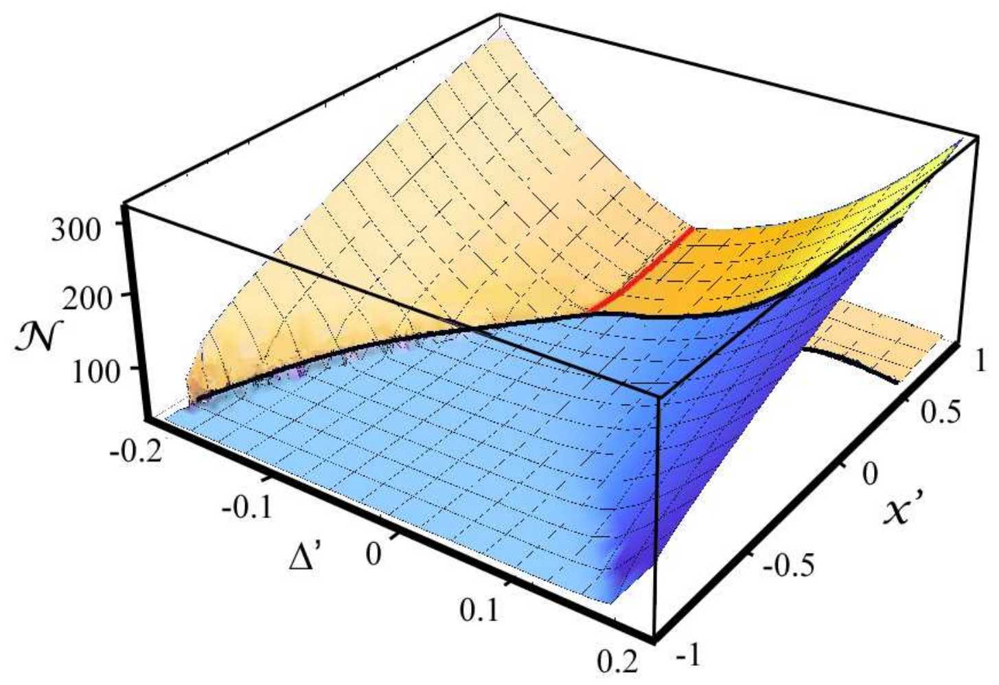
The values of shown correspond only to stable regimes of oscillations. The line of bifurcation points separates the () domains with and without bistability in Fig. 5. In the domain of bistability the higher and lower values of coincide along the red line. Away from the red line the high- and the low- values differ very strongly. High- values correspond to the regime of oscillations with frequency close to , see Fig. 3, whereas low -values correspond to the frequency of oscillations close to .
At and to the right from the bifurcation line there is no bistability. The value of is low in this domain around . As increases, grows for both signs of detuning, . However, for (blue detuning) the growth of is monotonical. At the same time, for (red detuning) the bistability sets in at certain critical . Upon further increase of the low- value does not grow, while the high- value grows rapidly.
It is instructive to compare the results shown in Fig. 5 to the results of Refs. [15, 16]. The curves were obtained in Refs. [15, 16] by numerical solution of the system of master equations for the density matrix describing both the two-level system and the oscillator. Firstly, there is a qualitative agreement in the shape of the boundary of bistability. In Refs. [15, 16] only the low- values are plotted. The prime observation made in Refs. [15, 16] was that there is a strong difference between these low- values for blue and red detunings, namely, for blue detuning is much higher. Our analytical results in Fig. 5 agree qualitatively with this observation.
VI Concluding remarks
Frequency, , of the Rabi oscillations is proportional to the square root of the excitation power. This linearity has been demonstrated in many experiments. Even when Rabi oscillations are damped, the dependence can be extracted from the position of maximum in the Fourier transform[20] of the signal, . We predict that, for a two-level system coupled to a vibrational mode, the position of maximum of the Fourier transform will deviate from the linear behavior near the resonance . Both to the left and to the right from the resonance the position of maxim corresponds to . The relative width of the resonant region depends on the coupling, , to the vibrational mode as . We also predict that, in the vicinity of the resonance, the dependence exhibits a hysteretic behavior with two stable values of corresponding to two stable regimes of the Rabi oscillations.
The underlying physics of the Rabi-vibronic resonance is the following. Without coupling, population inversion, , and displacement, , satisfy the harmonic oscillator equations with frequencies and , respectively. With coupling, two-level system acts as a driving force on the oscillator, while the back-action of the oscillator on is peculiar. The structure of back-action force is , as can be seen from Eqs. (8), (9). This structure implies that back-action is of a parametrical type, i.e., adds to . Thus, at , it appears that is modulated with frequency . This, however, does not lead to a parametric instability. Instead, the oscillator motion gets synchronized with the Rabi oscillations. In this regard, there is certain analogy to the synchronization of the Rabi oscillations to a sequence of pulses [21] applied to the detector with repetition period chosen to be .
As it was pointed out in Introduction, the situation when a two-level system undergoing the Rabi oscillations is coupled to the oscillator is actively studied in connection to the circuit QED[11]. The most common situation in circuit QED is when the oscillator frequency, , is tuned to the transition frequency, , of the two-level system. Among physical effects predicted for this domain is that two or multiple qubits can get strongly coupled to each other via coupling to a common oscillator[22, 23]. Rabi-vibronic resonance corresponds to the domain . Still the effects similar to those discussed in Refs. [22, 23] will take place under the conditions of the Rabi-vibronic resonance. In particular, we anticipate that Rabi oscillations in two driven two-level systems with , coupled to the same oscillator will get synchronized.
As a final remark, classical treatment of the vibrational mode adopted in the present paper does not allow one to capture the quantum jumps[17] between the stable regimes of collective motion of the two-level system coupled to the oscillator. We also did not consider the effect of thermal noise which leads to the activated switching[24] between the steady regimes even within a classical description of the oscillator.
Acknowledgements.
We are grateful to C. Böhme for a discussion which initiated this study. We thank J. Koch and F. von Oppen for bringing Refs. [15, 16] to our attention. We also acknowledge discussions with E. G. Mishchenko, O. A. Starykh, and B. Spivak, and the support of the Grant DMR-0808842 (R.G).References
- [1] I. I. Rabi, Phys. Rev. 51, 652 (1937).
- [2] E. T. Jaynes and F. W. Cummings, Proc. IEEE 51, 89 (1963).
- [3] L. Y. Gorelik, A. Isacsson, M. V. Voinova, B. Kasemo, R. I. Shekhter, and M. Jonson, Phys. Rev. Lett. 80, 4526 (1998).
- [4] Ya. M. Blanter, O. Usmani, and Yu. V. Nazarov, Phys. Rev. Lett. 93, 136802 (2004).
- [5] C. Galland and A. Imamoglu, Phys. Rev. Lett. 101, 157404 (2008).
- [6] C. Galland, A. Högele, H. E. Türeci, and A. Imamoglu, Phys. Rev. Lett. 101, 067402 (2008).
- [7] I. Wilson-Rae, C. Galland, W. Zwerger, and A. Imamoglu, e-print arXiv:0911.1330 (2009).
- [8] J.-J. Li, W. He, and K.-D. Zhu, Phys. Rev. B 83, 115445 (2011).
- [9] R. B. Capaz, C. D. Spataru, S. Ismail-Beigi, and S. G. Louie, Phys. Rev. B 74, 121401 (2006).
- [10] P. Avouris, M. Freitag, and V. Perebeinos, Nat. Photon. 2, 341 (2008).
- [11] see J. Schoelkopf and S. M. Girvin, Nature (London) 451, 664 (2008), and references therein.
- [12] E. Il’ichev, N. Oukhanski, A. Izmalkov, T. Wagner, M. Grajcar, H. G. Meyer, A. Y. Smirnov, A. Maassen van den Brink, M. H. S. Amin, and A. M. Zagoskin, Phys. Rev. Lett. 91, 097906 (2003).
- [13] V. I. Shnyrkov, D. Born, A. A. Soroka, and W. Krech, Phys. Rev. B 79, 184522 (2009).
- [14] A. Yu. Smirnov, Phys. Rev. B 68, 134514 (2003).
- [15] J. Hauss, A. Fedorov, C. Hutter, A. Shnirman, and G. Schön, Phys. Rev. Lett. 100, 37003 (2008).
- [16] S. André, V. Brosco, M. Marthaler, A. Shnirman, and G. Schön, New J. Phys. 10, 095018 (2008).
- [17] O. V. Zhirov and D. L. Shepelyansky, Phys. Rev. Lett. 100, 014101 (2008).
- [18] Ya. S. Greenberg, E. Il’ichev, and A. Izmalkov, Europhys. Lett. 72, 880 (2005).
- [19] Ya. S. Greenberg, Phys. Rev. B 76, 104520 (2007), Ya. S. Greenberg, E. Il’ichev, and F. Nori, Phys. Rev. B 80, 214423 (2009).
- [20] D. R. McCamey, K. J. van Schooten, W. J. Baker, S.-Y. Lee, S.-Y. Paik, J. M. Lupton, and C. Boehme, Phys. Rev. Lett. 104, 017601 (2010).
- [21] A. N. Korotkov, Phys. Rev. B 83, 041406 (2011).
- [22] J. Majer, J. M. Chow, J. M. Gambetta, J. Koch, B. R. Johnson, J. A. Schreier, L. Frunzio, D. I. Schuster, A. A. Houck, A. Wallraff, A. Blais, M. H. Devoret, S. M. Girvin, R. J. Schoelkopf, Nature 449, 443 (2007).
- [23] M. Dukalski and Ya. M. Blanter, Phys. Rev. A 82, 052330 (2010).
- [24] M. I. Dykman and M. A. Krivoglaz, Zh. Eksp. Teor. Fiz. 77, 60 (1979) [Sov. Phys. JETP 50, 30 (1979)].