Three Body Resonance Overlap in Closely Spaced Multiple Planet Systems
Abstract
We compute the strengths of zero-th order (in eccentricity) three-body resonances for a co-planar and low eccentricity multiple planet system. In a numerical integration we illustrate that slowly moving Laplace angles are matched by variations in semi-major axes among three bodies with the outer two bodies moving in the same direction and the inner one moving in the opposite direction, as would be expected from the two quantities that are conserved in the three-body resonance. A resonance overlap criterion is derived for the closely and uniformly spaced, equal mass system with three-body resonances overlapping when interplanetary separation is less than an order unity factor times the planet mass to the one quarter power. We find that three-body resonances are sufficiently dense to account for wander in semi-major axis seen in numerical integrations of closely spaced systems and they are likely the cause of instability of these systems. For interplanetary separations outside the overlap region, stability timescales significantly increase. Crudely estimated diffusion coefficients in eccentricity and semi-major axis depend on a high power of planet mass and interplanetary spacing. An exponential dependence previously fit to stability or crossing timescales is likely due to the limited range of parameters and times possible in integration and the strong power law dependence of the diffusion rates on these quantities.
1 Introduction
The stability of multiple planet systems has been long been a matter of interest as it concerns the long term stability of the Solar system. Poincaré noticed that perturbation techniques involved singularities or small divisors that prevented solution by convergent series. Recent numerical explorations suggest that the giant planets in our solar system were originally located in a more compact location and experienced a subsequent planet-planet scattering event (within the context of the “Nice model”; Tsiganis et al. 2005). All extrasolar planetary systems may experience epochs of dynamically instability (e.g. Ford et al. 2001; Barnes & Greenberg 2006; Chatterjee et al. 2008; Thommes et al. 2008; Gozdziewski & Migaszewski 2008; Gozdziewski & Migaszewski 2009; Raymond et al. 2009a; Kopparapu & Barnes 2010; Fabrycky & Murray-Clay 2010).
Numerical integrations show that a system of two planets on initially zero-inclination and eccentricity orbits about a star never experience mutual close encounters if the initial semimajor axis separation is sufficiently large (Marchal & Bozis, 1982; Gladman, 1993; Barnes & Greenberg, 2007), (also see Mardling 2008). Stability of multiple planet systems is often discussed in terms of this limit which has been called “Hill stability” (e.g., Marchal & Bozis 1982; Barnes & Greenberg 2007; Raymond et al. 2009b). Systems with multiple planets or satellites are stable over long periods of time if the bodies are sufficiently distant from each other (Chambers et al., 1996; Duncan & Lissauer, 1997; Faber & Quillen, 2007; Chatterjee et al., 2008; Smith & Lissauer, 2009). For an integration begun with all bodies at zero eccentricity and inclination, the integration time until one body crosses the orbit of an other body is known as a crossing timescale, . We refer to the idealized problem studied by Chambers et al. (1996) with equal mass planets and with the semi-major axis of each consecutive planet set from that of the previous one using a constant ,
| (1) |
The planets have mass ratio with respect to the central star . When the planet number is greater than five, the crossing timescale is insensitive to the number of bodies (e.g., Chambers et al. 1996).
A number of studies have fit power laws to the crossing or stability timescale. Duncan & Lissauer (1997) found that the crossing time is sensitive to the mass of the satellites with where is a slope and is an offset. Chambers et al. (1996) found , whereas Smith & Lissauer (2009) fit . Here the parameters , are fit to the numerically measured crossing timescales and are not identical in each setting. These numerical studies integrated for timescales between 100 and orbital periods of the innermost orbiting body. The interplanetary separation ranged from 1 to about 10 mutual Hill radii and the mass ratio ranged from to . The trends in the numerically measured crossing timescales are currently lacking an explanation.
The power law forms for the crossing timescales can be re-written for exponents (Faber & Quillen, 2007). The exponential form is reminiscent of the Nekhoroshev theorem (Nekhoroshev, 1977) or of Arnold diffusion (Arnold, 1962) in the context of weakly perturbed Hamiltonian systems. There are subtle and deep connections between the Nekhoroshev theorem and Arnold diffusion (e.g, as explored and discussed by Chirikov 1979; Lochak & Neishtadt 1992; Lochak 1993). Arnold diffusion takes place on exponentially long timescales whereas systems with resonances that are fully overlapped can have relatively faster diffusion rates. This led Morbidelli & Froeschlé (1995) to suggest that systems with sparse and weak resonances might exhibit diffusion on exponentially long timescales whereas those affected by multiple and overlapping resonances would diffuse at a rate that depends on a power law of time (also see Guzzo et al. 2002). A number of studies have numerically measured a power law relation between Lyapunov and instability or crossing timescales (Lecar et al., 1992; Levison & Duncan, 1993; Murison et al., 1994; Morbidelli & Froeschlé, 1995; Mikkola & Tanikawa, 2007; Urminsky & Hegge, 2009; Shevchenko, 2010) suggesting that the stability or crossing timescales are driven by chaotic diffusion or Hamiltonian intermittency. Because there is a power law relation between Lyapunov and crossing timescales, we would expect that the diffusion rate would be a power law function of the perturbation parameters (such as planet mass and planetary separation) rather than an exponential function of them as commonly fit. This apparent contradiction has been discussed in terms of two regimes for the dynamics, a weakly perturbed “Nekhoroshev” regime exhibiting diffusion over exponentially long timescales and a resonant overlap power law regime exhibiting diffusion at a rate that depends on a power of the perturbations (Morbidelli & Froeschlé, 1995).
In this study we consider the role of three-body resonances in the idealized setting studied by Chambers et al. (1996) of a closely and uniformly spaced equal mass co-planar system initially in nearly circular orbits. Our goal is to understand the dynamics of the idealized coplanar, closely and uniformly spaced equal mass multiple planet system sufficiently well that we can identify the source of instabilities in multiple planet systems. Previous studies of three-body resonances have primarily focused on settings where one of the bodies is small, such as an asteroid perturbed by both Jupiter and Saturn (Murray et al., 1998; Nesvorny & Morbidelli, 1999; Guzzo, 2005) but also include the early study of the Laplace resonance by Aksnes (1988). While three-body resonances are weak there are more of them than two-body resonances so they can be a source of chaotic behavior causing slow diffusion in eccentricity and inclination (Nesvorny & Morbidelli, 1998; Nesvorny & Morbidelli, 1999; Guzzo et al., 2002; Guzzo, 2005). Three body resonances may be important in extra solar multiple planet systems. The long-term stability of extra solar multiple planet systems may be influenced by a net of low order two and three-body resonances (Gozdziewski & Migaszewski, 2008; Gozdziewski & Migaszewski, 2009; Fabrycky & Murray-Clay, 2010).
We first estimate the strength and libration frequency in zero-th order (in eccentricity) three-body resonances. Conserved quantities for them are also estimated so that their signature in numerical integrations can be identified. Using estimated numbers and widths of the three-body resonances we derive a resonance overlap criterion. In the final section we discuss the role of three-body resonances in causing instability in multiple planet systems and whether they may eventually provide an explanation for the exponential forms fit to their crossing timescales.
2 Hamiltonian for a Multiple Planet system
2.1 Non-interacting System
The Hamiltonian for non-interacting massive bodies orbiting a star (and so feeling gravity only from the star) can be written
| (2) |
where is the mass of the -th body (or planet) divided by the mass of the star, . Here we have ignored the motion of the star and have put the above Hamiltonian in units such that where is the gravitational constant. Here the Poincaré coordinate , where the semi-major axis of the -th planet is . This Poincaré coordinate is conjugate to the mean longitude, of the -th body. The mean longitude where is the mean anomaly and is the longitude of pericenter of the -th body. We may also use the Poincaré coordinate where is the -th body’s eccentricity. This coordinate is conjugate to the angle . We will restrict our system so that all planets are orbiting in the same plane and so will begin by ignoring the Poincaré coordinates associated with inclination and the longitude of the ascending node. Each Poincaré momenta contains a factor of a planet’s mass. Some studies of three-body resonances have focused on the problem of a low mass object in the presence of two planets (e.g., an asteroid perturbed by Jupiter and Saturn; Nesvorny & Morbidelli 1998; Murray et al. 1998) and so have removed the mass from the Poincaré momenta associated with the low mass object.
2.2 Interactions
We now consider the gravitational interactions between the planets. Here we consider only the direct term and ignore the indirect terms. The Hamiltonian can be written
| (3) |
where the interaction term, , is a sum of direct interaction terms, , and
| (4) |
If the planets are in nearly circular orbits
| (5) |
and we have assumed that and
| (6) |
We can expand in Fourier components
| (7) |
with coefficients
| (8) |
where is a Laplace coefficient,
| (9) |
Laplace coefficients are the Fourier coefficients of twice the function . As this function is locally analytic the Fourier coefficients decay rapidly at large and the rate of decay is related to the width of analytical continuation in the complex plane. This function can be analytically continued on the complex plane in the region with . The Cauchy root test for convergence implies that in the limit of large that and so the Fourier coefficients decay rapidly. We approximate Laplace coefficient with the function
| (10) |
where is the interplanetary separation (equation 1) and . This Laplace coefficient diverges logarithmically for small (or for near 1) and drops exponentially at large . In Figure 1 we graphically show this approximation for the Laplace coefficient for in the range 0.2 to 0.01.

We can write the interaction term as a function of Poincaré coordinates.
| (11) |
Indirect terms can be neglected here because they only contribute a single zero-th order Fourier component, that with (e.g., see appendix Table B.2 by Murray & Dermott 1999).
3 Three body resonances
We consider the possibility that the system is not in any two body resonances where with integers , but might be in a three body resonance. Here is the mean motion of the -th body. A Laplace relation exists between three orbiting bodies if the frequency
| (12) |
Integrating the previous equation (and assuming that the precession rates are slow) we find that the angle
| (13) |
This angle librates about a particular value (often 0 or ) when in a three-body resonance. The period, , corresponds to the time between successive repetitions of the initial configuration
| (14) |
We try to maintain the ordering and .
We explore how 3-body interaction terms involving angles such as given in equation (13) can be constructed from individual 2-body interaction terms. A similar procedure has been used before to estimate 3-body resonance strengths (Aksnes, 1988; Nesvorny & Morbidelli, 1998; Murray et al., 1998; Nesvorny & Morbidelli, 1999; Guzzo, 2005) (also see Chirikov 1979). Our procedure is to carry out a first order canonical transformation that is designed to remove the two 2-body interaction terms. The procedure is described, for example, in section 4.1 by Ferraz-Mello (2007).
3.1 Canonical transformation removing first order (in mass) two-body interaction terms
We begin with the Hamiltonian for three bodies, lacking indirect terms and with two Fourier components from two separate two-body interaction terms. We first consider zero-th order components (in eccentricity) so we need only consider the Poincaré coordinates where the vectors refer to the the coordinates and momenta for three planets. We chose two components with arguments (angles) whose difference is equal to a three-body Laplace angle (equation 13)
Our Hamiltonian with these two components
| (15) | |||||
with the functions
| (16) |
as discussed in the previous section. We have used the notation
It is useful to compute some derivatives
| (17) |
with . We can use the shorthand
| (18) |
and similarly with indices .
We use a generating function with new momenta and old coordinates
| (19) | |||||
to generate a canonical transformation. Here is a function of and and similarly . This canonical transformation is designed to remove the two perturbation terms in the Hamiltonian to first order in the planet masses. Derivatives of the generating function give us new coordinates in terms of the old ones
| (20) | |||||
It is useful to relate
| (21) |
and similarly for the other bodies.
We replace our old coordinates and momenta with new ones in the Hamiltonian finding that in the new coordinates the first order two body terms have been removed by the transformation. We expand to second order in the masses and find that the Hamiltonian has gained second order terms. During this procedure we drop terms that depend on , or and , or while keeping those containing the products and . We rewrite these products in terms of the sum and difference of the angles and discard the term that contains the sum of the angles so as to retain only the term that depends on the Laplace angle . When the Laplace angle is slowly varying (and the system is near a three-body resonance) the other terms are rapidly varying and so can be neglected.
| (22) |
with
| (23) | |||||
Our procedure using a canonical transformation should give a resonance term equivalent to the zero-th order term derived by Aksnes (1988) using Lagrange’s equations, though it is not easy to check because of the differences in notation. The resonance term is zero-th order in planet eccentricity but second order in the planet masses. Hereafter we drop the primes in the coordinates.
The full Hamiltonian contains additional two-body terms however the angles involved are expected to vary quickly compared to . Neglecting fast angles is equivalent to averaging over them. Equivalently as long as there are no combinations that yield slow angles, the other interaction terms may be removed using near identity canonical transformations similar to that used above.
3.2 Width, libration frequency and conserved quantities for the zero-th order three-body resonance
The Hamiltonian (equation 22) that contains a three-body term can be used to estimate the width and timescales in a Laplace resonance. We can perform a canonical transformation to reduce the dimension of the problem. Consider the generating function
| (24) |
leading to new angles
| (25) |
and new momenta such that
| (26) |
After the transformation, the new Hamiltonian (using equation 22) is
| (27) | |||||
The new Hamiltonian only depends on the angle and does not depend on the two longitudes (that are unchanged by the canonical transformation) so the two conjugate momenta are conserved quantities. Our conserved quantities can be written as
| (28) |
Differentiating these conserved quantities with respect to the semi-major axes we find that small changes
| (29) |
These derivatives imply that a small change in semi-major axis by one body will be mirrored by changes in semi-major axis of the two other bodies. The signs imply that the outer two bodies move in the same direction but the middle one moves in the opposite direction. The middle body is expected to move more than the outer two as we expect is greater than and . This behavior can be seen in particle integrations as we will discuss below.
We can expand the momentum about an initial value. Consider initial values for corresponding to initial value , conserved quantities , initial semi-major axes and mean motions
| (30) |
We define
| (31) |
and expand the Hamiltonian (equation 27) about . To second order in
| (32) |
where the constant contains terms that depend on our conserved quantities () and . The coefficients
| (33) |
The coefficient is also evaluated at . We can think of the coefficient as a product
| (34) |
setting distance to resonance, where the vector of integers
| (35) |
On resonance . The coefficient depends approximately on the magnitude of the vector with .
With a shift in the momentum, , the Hamiltonian (equation 32) can be written so as to remove the term that is proportional to ,
| (36) |
We estimate the width of the resonance in momentum is
| (37) |
corresponding to a resonant width in Poincaré momentum of
| (38) |
(using equation 26) and a width in terms of semi-major axis of the innermost body
| (39) |
A jump across resonance would give a change for the inner body. Using equations (29) changes in semi-major axis for the other two bodies can be estimated from that of the inner one.
The libration frequency in the resonance is
| (40) |
For a system initially with to be in resonance we require that the shift, , (relating and ) is smaller than half the resonance width ( in equation 37). Using this condition and equations (37) and (40) we require to be near or in resonance or using equation (34)
| (41) |
3.3 Estimates of three-body resonance strengths and frequencies for closely and evenly spaced equal mass multiple planet systems
We consider the strength of the various terms contributing to the Laplace resonance strength, in equation (23), for a closely and evenly spaced equal mass system. For the equally spaced system (represented by equation 1) . In this setting the only Laplace angles that can be nearly fixed have about the same size as . We work in units of the mean motion and semi-major axis of the innermost body involved in the three-body resonance. Differences in the mean motions can be approximated as
| (42) |
where
| (43) |
As the Laplace coefficient can be approximated given in equation (10), the derivatives of the Laplace coefficients can be approximated as
| (44) |
(using ). Using these approximations and assuming equal masses, we find that the interaction term strength in equation (23) is approximately
| (45) | |||||
where we have assumed integers are positive. The terms all have the same sign and in most cases the first term dominates so we can approximate the interaction strength as
| (46) |
Note that is positive, so we would expect libration around Laplace angle of zero or
| (47) |
For (corresponding to being near resonance for small ) we estimate that (using equation 33) and from equation (40) and equation (46) the libration frequency in the resonance is approximately
| (48) |
The width of the resonance (in terms of momentum ; equations 38, 39) gives a width in semi-major axis similar in size or
| (49) |
where we have assumed and so neglected the exponential. The above equation should give the size of jumps across resonance for the inner body.
Likely equation (49) somewhat underestimates the resonance widths as we have not taken into account all terms in equation (23). We have also neglected the dependence of on the momentum in our estimates of (equation 40) and (equation 39). The conserved quantities in resonance imply that increases when decreases and vice-versa, so may not be strongly dependent on .
Because the Laplace coefficients drop exponentially with separation (see Figure 1) or the distance between the planets, resonances between the first, second and fourth bodies or other non-consecutive combinations should be much weaker than those involving three consecutive bodies. However if the masses of the bodies differ then three-body resonances involving non-consecutive triplets could be important.
3.3.1 First order resonances
Zero-th order (in eccentricity) resonances do not influence the Poincaré variable associated with eccentricity so they should not affect planet eccentricities. First order three-body resonances (as previously considered by Aksnes 1988) have interaction terms in the form
| (50) |
with a single longitude of pericenter . The longitude of pericenter can be that of any of the three planets involved in the resonance, so that can be equivalent to or . Because the interaction term contains a longitude of pericenter it can affect a planet’s eccentricity. The strength can be estimated in the same way as we have estimated the zero-th order three-body resonance strengths but instead of carrying out a transformation with two zero-th order two-body interaction Fourier terms, one begins with a zero-th order and a first order two-body Fourier term.
When expanded to first order in planet eccentricity and inclination the two-body interaction terms (equation 4) gain Fourier components (that would be added to equation 7)
| (51) |
where
and coefficients
| (53) |
(equation 6.107 Murray & Dermott 1999; also see Tables B.4 and B.7). An approximation to these coefficients is shown in Figure 2. Also .
First order and zero-th order terms when combined form a term with a three body argument similar to that shown in equation (50). We list below on the left the two Fourier components that when combined give the argument on the right;
The longitude of pericenter in the argument determines the eccentricity related Poincaré coordinate. For example, if the argument contains then the three-body term contains a factor of and similarly for bodies .

Whereas the zero-th order three-body resonances involve two coefficients, the first order three-body resonances involve a single and a single coefficient. The coefficients are approximately derivatives of the coefficients. The strength, , of the first order three-body term we expect is larger than by a factor of because it would involve an extra derivative of the Laplace coefficient. However the dependence on the Poincaré coordinate associated with the eccentricity can reduce the strength of the resonance. The first few conjunctions of an initially zero eccentricity system lead to planet eccentricities of order a few times (e.g., equation 10.57 Murray & Dermott 1999). This suggests that the ratio of the first to zero-th order resonance strengths is approximately . It may be convenient to define where is the Hill radius of the planet. The ratio of resonance strengths is then approximately , or the interplanetary separation in units of the planet’s Hill radius. For eccentricities above a critical value (e.g., set dimensionally; Quillen 2006) the resonant width and libration frequency depends on the square root of . As is in the range –10 for the systems studied numerically (e.g., Chambers et al. 1996; Smith & Lissauer 2009) we expect that first order resonances are initially a few times weaker than the zero-th order ones. However, a system evolving in multiple three-body zero-th order resonances can cross first order resonances causing variations in planet eccentricities. Because of the number of possible angular combinations there are more first order resonances than zero-th order ones.
4 Three-body resonances as seen in a numerical integration
In Figure 3 we show a numerical integration of 5 equal mass bodies initially in a coplanar circular orbits about a central star. The ratio of the planet masses to that of the central star is . The initial separation between the bodies is given by using equation (1). The numerical integration was done using the hybrid algorithm of the code Mercury version 6.2 (Chambers, 1999). Time is given in units of the initial rotation period of the inner body. Distances are given in units of the inner body’s initial semi-major axis. This numerical integration was chosen to illustrate phenomena associated with three-body resonances and we will use it to check predicted sizescales for them. For these parameters and . In terms of the mutual Hill radius (as defined by equation 1 by Smith & Lissauer 2009) , placing it in the middle of the regime studied by Smith & Lissauer (2009) though they primarily considered planets lower in mass by a factor of 3. This separation places our integration at larger separations than the mean explored by Chambers et al. (1996) (on the right hand side of the top panel of their Figure 3) with a crossing timescale of about orbital periods.
In Figure 3a we show the semi-major axes of the 5 bodies. Variations in semi-major axis often involve similar motions for three consecutive bodies, with the inner and outer ones (of this triplet) moving together and the central one of the triplet moving in the opposite direction. This is expected as in a three-body resonance there are two conserved quantities (equations 28) that relate variations in semi-major axes between the three bodies (equations 29). Figure 3b shows the Laplace angles for . We can write with . The angle is plotted for the inner three consecutive bodies (bottom panel), the middle three consecutive bodies (middle panel) and the outer three consecutive bodies (top panel), respectively. Figure 3c is similar but for the resonances with . We see from Figures 3b,c that there are times when specific Laplace angles vary slowly or vibrate about 0 or . The system is affected by more than one Laplace resonance. At some times the inner three bodies move together, and at other times the middle or outer three move together. For example, the variations in the outer three planets at periods are likely due to the resonance involving the outer three bodies. Variations in the inner three planets at are likely due to the resonance involving the inner three bodies. When the Laplace angle ceases to circulate and librates about 0 or we see that variations in the three planets involved in the Laplace resonance are related, with the outer two increasing or decreasing in semi-major and the middle one moving in the opposite direction. The middle body experiences larger variations in semi-major axis as would be expected from the conserved quantities (see equations 28 and 29). We have checked that the conserved quantities in these resonances do not make large variations when the resonant angle is not rapidly circulating. However, conserved quantities associated with one resonance can vary while a different resonance is affecting the system.
For and a jump across resonance should give a change in semi-major axis for the inner body (using equation 49) of approximately . Jumps seen in the simulation (Figure 3a) are a factor of a few larger than this. We can consider this moderately reasonable agreement as we have only made rough estimates of the resonance properties. The libration frequency in the resonance (computing using equation 48) is approximately corresponding to a period of years. This period is short enough that the slow variations in angle in Figures 3a,b can be attributed to the three-body resonances.
The simulation shown in Figure 3 is affected simultaneously by more than one zero-th order three-body resonance (here and resonances and for three possible consecutive triplets of planets) suggesting that they are dense and wide enough that the three-body resonances overlap. If so then random variations in semi-major axis can be attributed to chaotic behavior associated with multiple resonances.
For the same numerical integration we also show the eccentricity evolution in Figure 4a. This figure also plots angles for and . These angles are not in the form as the sum of the indices in the vector is not zero. First order (in eccentricity) thee-body resonances involve a single planet’s longitude of pericenter, for example, the angle could be one of the following
| (55) |
These angles arise from combining a zero-th order two-body term with a first order two-body term. As the precession rates, , are slow compared to the mean motions, we have plotted angles omitting a longitude of pericenter. We have examined similar plots containing all of the above possible angular combinations and found that they are similar to but noisier than Figures 4b,c. Since the planet eccentricities are low, small variations in the orbits can give large changes in the computed longitudes of pericenter.
From Figure 4b,c we see that our numerical integrations also exhibit slow angles associated with first order three-body resonances. When first order resonances are crossed we expect small changes in planet eccentricity. For example at the inner three planets are affected by the resonance leading to an increase in eccentricity in these three planets. At years the outer three planets are affected by the resonance leading to an increase in the eccentricity of the fourth planet. Jumps in eccentricity seem similar in size to those of jumps in semi-major axis though we expected them to be a few times smaller based on the discussion in section 3.3.1. A comparison between the angles shown in Figure 3b and Figure 4b shows that they are very similar; likewise for Figure 3c and Figure 4c. Hence the zero-th order resonances (with angles shown in Figure 3b,c) overlap the first order resonances (with angles shown in Figure 4b,c).
Once the eccentricity of a planet is increased secular perturbations cause oscillations in the eccentricities of the nearby bodies. By summing the eccentricities of all the planets it is possible to average over the secular oscillations. The smoothed sum of the planet eccentricities shown in the top subpanel of Figure 4a shows locations where stronger jumps in eccentricity of the entire system occur and these correspond to times when first order resonances are affecting the system. We can interpret the slow increases in planet eccentricity during the integration as due to first order three-body resonances. This follows as the zero-th order resonances should not affect the eccentricities and there are no strong nearby two-body resonances. As the system wanders in semi-major axis first order three-body resonances are crossed leading on average to the slow eccentricity evolution evident in Figure 4a.


5 Resonance Overlap Criterion
We consider whether the number density and widths of three-body resonances are sufficient that they are likely to overlap. We estimate the number density of three body resonances and multiply this by the width of the resonances. The result is a filling factor that if greater than 1 implies that the three-body resonances overlap and so can induce chaotic behavior in the system. The ‘resonance overlap criterion’ for the onset of chaotic behavior was pioneered by Chirikov in 1959 (see Chirikov 1959; Chirikov 1979; Lichtenberg & Lieberman 1992). A similar approach has been used to estimate the width of the chaotic zone near a planet’s corotation resonance (Wisdom, 1980; Murray & Holman, 1997; Quillen & Faber, 2006) and the onset of chaotic behavior in other settings (Chirikov, 1979; Holman & Murray, 1996; Mudryk & Wu, 2006; Mardling, 2008). Three-body resonance overlap has been seen in numerical studies of the outer Solar system (Guzzo, 2005).
Each zero-th order three body resonance is specified by two integers and three consecutive planets. Given a particular value we can first consider the separation between the three-body resonances with different values. We consider an equally spaced system with separation set by . Let be the ratio of mean motions between consecutive planets . The vector of mean motions for three consecutive planets and distance to resonance (equations 33, 34). This gives . Solving for when we find that on resonance . We can differentiate this with respect to to find the distance between resonances. Given a value for , the distance between resonances with adjacent values (in terms of differences in mean motions or in terms of differences in ) is of order . For small , is near 1 and so on resonance . Consequently the number density of three body resonances with is (and estimated from the separation ) is
| (56) |
The number density is approximately in units of the mean motion of the innermost body involved in the resonance.
We now consider the width of each resonance. Consider where is on resonance with . We estimate the distance to resonance (equations 33, 34)
| (57) |
To be near or within the resonance (determined by the condition given in equation 41 or distance to resonance is smaller than times the libration frequency)
| (58) |
or
Here we have used equation (48) for the libration frequency. Multiplying by a factor of two so as to cover both sizes of resonance and assuming appropriate for resonances when is small, the resonant width (corresponding to a range in or ) is
| (59) |
We combine the resonant width with the number density to estimate a three-body resonance filling factor. For each the number density of resonances times their width is
| (60) |
To estimate the total filling fraction, , of three-body resonances we integrate the previous expression over all possible values;
| (61) | |||||
When the zero-th order three-body resonances are sufficiently numerous and wide that they are likely to overlap.
For the simulation shown in Figure 3 we compute placing the system near the regime of resonance overlap. This is perhaps not surprising as we found that the system was influenced by both the and resonances. Inverting the above equation with we find that resonance overlap occurs when
| (62) |
The form of the criterion may be related to the slopes for stability or crossing timescales measured by Chambers et al. (1996).
Were we to take into account the possible combinations of consecutive planets (e.g, for there are three groups of consecutive planets) and first order resonances, the modified filling factor would be somewhat larger than computed in equation (61). We expect the first order resonances to initially be weaker than the zero-th order resonances but because of the additional possible angle combinations there there are few times more of them. Consequently first order resonances may contribute to the overlap criterion. A more accurate criterion would likely cover the regime integrated by numerical studies where the separation ranges from 0.5 – 4 (e.g., Chambers et al. 1996). The exponential dependence in the Laplace coefficient on interplanetary distance (equation 10) implies that three-body resonances for non-consecutive combinations of planets are unlikely to be strong. This explains why the crossing or stability timescale for equidistant closely spaced systems is only weakly dependent on the number of planets when the number (Chambers et al., 1996). The resonance overlap criterion suggests that there is a critical separation value that separates two regimes, an inner one at small governed by instability from overlapping three-body resonances and an outer one that is much more stable. Two separate regimes and a transition from one to another at larger separations does seem to be exhibited in numerical integrations (Smith & Lissauer, 2009). As there are fewer combinations of consecutive planets for low we would expect this transition would occur at smaller separations; this too is seen in numerical integrations (Figure 13 by Smith & Lissauer 2009).
6 Crude Estimates for Diffusion
We expect that the resonances that overlap would often be similar in size, as illustrated in the integration shown in Figure 3 where the and three-body resonances were both important. Assuming full resonance overlap, we estimate a diffusion coefficient for wander in the Poincaré coordinate
| (63) |
where we use equation (38) for the changes in and have assumed that these changes take place on a timescale equal to the libration frequency (equation 40). This type of estimate is similar to those explored by Chirikov (1979). Using approximations for these quantities (equations 48 and 33) we estimate
The diffusion coefficient is largest for the highest value which has because the Laplace coefficients drop exponential at higher p. Setting
| (64) |
corresponding to a diffusion coefficient in semi-major axis of
| (65) |
An upper limit for a crossing timescale would be the time it takes for the semi-major axis to wander a distance approximate equal to the interplanetary spacing or
| (66) |
Using our estimate for the diffusion coefficient this gives
| (67) |
For the system we show in Figures 3 and 4 this corresponds to years, and about 3 orders of magnitude greater than expected from the fit to the crossing timescales (Faber & Quillen, 2007) or inferred from Figure 3 by Chambers et al. (1996). Consequently this timescale severely overestimates the crossing timescales.
It is likely the eccentricity evolution must be considered as even small increases in eccentricity can strongly affect the stability or crossing timescales (Zhou et al., 2007). There are many first order three-body resonances but eccentricity increases due to them are very small. There are fewer two-body first order resonances but eccentricity increases due to them could be high if the system wanders into one. The minimum eccentricity of a body in the vicinity of a first order mean motion resonance scales with (e.g., Quillen 2006, table 1, or Mustill & Wyatt 2011). This is a small power, and so not small for the regime covered by numerical integrations that have interplanetary separations of order a few to a dozen Hill radii. We adopt the ansatz that the crossing timescale is set by the time it takes for the system to wander into a first order mean motion resonance among two consecutive bodies.
We first estimate the distance that one planet must wander (due to the three-body resonances) before it encounters a first order two-body mean motion resonance. In the limit of high , first order resonances (with mean motions with a ratio of ) are separated in semi-major axis by . For an interplanetary separation of the nearest first order two-body resonance likely has . Thus the distance between resonances is .
Using our above estimated diffusion coefficient for semi-major axis wander (equation 65), the time it takes to cross a first order two-body mean motion resonance due to wander in semi-major axis would be of order
| (68) |
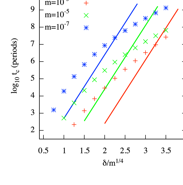
In Figure 5 we show a comparison between crossing times predicted with the above timescale and crossing times measured numerically. The numerically measured timescales are shown with the fit to the numerically measured value by Faber & Quillen (2007). This estimate is within two orders of magnitude of the relation found numerically and overestimates the crossing time at small separations. Nevertheless it is the first analytical derived estimate of crossing time that covers an appropriate range in parameter space. We note that because of the high power of in the above equation our power law relation is nearly as steep as the numerically measured times that have primarily been fit with exponential functions. On Figure 5 the resonance overlap boundary would be at a constant value of corresponding to a vertical line on the right hand side of this plot. Numerical integrations cover the range of shown in this plot hence we expect that the overlap criterion line should lie on the right hand side of the plot with . Our predicted location (equation 62) for the onset of three-body resonance overlap is about a factor of two or so too low as this line lies in the middle rather than the right hand side of the plot.
The above crude estimates for a diffusion coefficient (equation 64) and a crossing time (equation 68) are strong power law functions of both mass and interplanetary separation. Their strong dependence on separation suggests that the exponential forms fit to the numerically measured stability or crossing timescales (Chambers et al., 1996; Duncan & Lissauer, 1997; Zhou et al., 2007; Chatterjee et al., 2008; Smith & Lissauer, 2009) might in future be accounted for through chaotic motions induced by three-body resonances. Perhaps the exponential form has provided a good fit because of the limited range of times over which these systems can be integrated and because the diffusion rate is such a strong function of mass and separation. If three-body resonances overlap then there is no underlying mathematical reason (related to Arnold diffusion or the Nekhoroshev theorem) that would predict an exponential dependence on interplanetary separation and mass. We suspect that only outside the regime of three-body resonance overlap could a true long timescale exponential dependence on planet mass and separation be recovered.
7 Summary and Discussion
In this paper we have considered the role of three-body resonances for an idealized equal mass, uniformly spaced, but closely packed initially low eccentricity co-planar multiple planet system. We have estimated the strengths and libration timescales for zero-th order (in eccentricity) three-body resonances using an asymptotic approximation to the Laplace coefficient. Two conserved quantities are present relating variations in semi-major axes between the bodies affected by the resonance. These variations and the Laplace angles are useful for identifying the effect of three-body resonances in numerical integrations of multiple planet systems.
By estimating the number and widths of the three-body resonances, we have derived an approximate resonance overlap criterion. We find that zero-th order three-body resonances are likely to overlap when the separation between planets . The resonance overlap criterion is close to the regime covered by numerical integrations of multiple planet systems exhibiting instability (Chambers et al., 1996; Duncan & Lissauer, 1997; Zhou et al., 2007; Chatterjee et al., 2008; Smith & Lissauer, 2009), suggesting that the instability seen in integrations of closely spaced multiple planetary systems is due to chaotic behavior associated with multiple three-body resonances. We note that previous studies of asteroids have also attributed chaotic behavior to three-body resonances (Murray et al., 1998; Nesvorny & Morbidelli, 1998).
Our resonance overlap criterion lies near but within the regime covered by numerical integrations exhibiting instability implying that we have underestimated the filling factor of resonances by a factor of a few. However, we have not taken into account first order three-body resonances, the different combinations of consecutive planets, indirect terms in the Hamiltonian and we have only crudely estimated resonance strengths. Future works can improve upon the overlap criterion by expanding and improving the calculation.
For spacings larger than the overlap criterion boundary three-body resonances should not be as dense and the probability of resonance overlap drops. We postulate that there is a region of long timescale stability at large separations. This region and the transition between the two regimes is likely the reason for measured changes in slope of crossing time versus separation and a strong increase in crossing time at large separations (see Figures 1-4 by Smith & Lissauer 2009). The filling factor of three-body resonances should be lower for systems with fewer planets because there are fewer combinations of consecutive planets and so fewer strong three-body resonances. Thus we expect the transition to a more stable regime would occur at smaller planetary separations when there are fewer planets. This also is seen in numerical integrations (see red points in Figure 13 by Smith & Lissauer 2009).
We have attempted to predict diffusion rates using three-body resonances. The timescale to wander a distance of the interplanetary separation grossly overestimates the crossing timescale whereas that to diffuse until the system crosses a first order mean motion resonance between two bodies overestimates the crossing timescale by 1 or 2 orders of magnitude at small separations. This estimated timescale depends on the 8-th power of the interplanetary spacing suggesting that exponential functions have primarily been successful at fitting numerically measured crossing timescale because of the strong dependence on separation of the three-body resonances. Future work could strive to improve upon these gross estimates. Crossing timescales are not directly related to diffusion coefficients and the dynamics may be intermittent and diffusion anisotropic (e.g., Shevchenko 2010; Guzzo 2005). To better account for or predict the crossing timescales perhaps Lyapunov timescales and diffusion coefficients (i.e., eccentricity growth rates and rates of wander in semi-major axis) could be measured directly from numerical integrations. These then may be easier to understand with analytical estimates such as explored here.
Here we have considered equal mass, equidistant coplanar systems. However much of the framework developed here could be applied to less ideal systems such as closely spaced multiple planet extrasolar planetary systems. We remind the reader that here we have focused on systems that are in three-body resonances but are not in strong two-body resonances. Three body resonances may also be important in these systems but calculations are likely to be more challenging in this setting. Diffusion in semi-major axis seen in simulations of closely spaced satellite systems, e.g., the Uranian satellite system, (Duncan & Lissauer, 1997; Showalter & Lissauer, 2006; Dawson et al., 2010) and the Kepler 11 system (Lissauer et al., 2010) might in future be interpreted in terms of variations arising from three-body resonances.
Acknowledgements. This work was in part supported by NSF through award AST-0907841. We thank the Isaac Newton Mathematical Institute for hospitality and support during the fall of 2009 where this work was begun.
This work could not have been carried out without helpful discussions with Pierre Lochak, Ivan Shevchenko, J.-L. Zhou, Eric Ford, Adam Lanman, and Rob French.
I thank the referee for a thorough and careful reading of this manuscript leading to many corrections in calculation.
References
- Aksnes (1988) Aksnes, K. 1988, General formulas for three-body resonances, in “Long-Term Dynamical Behaviour of Natural and Artificial N-body Systems”, ed. A. E. Roy, (Kluwer Academic Publishers, Dordrecht), 125
- Arnold (1962) Arnold, V. I. 1962 Dokl. Akad. Nauk SSSR 156, 11 (with translation in 1964, Sov. Math. Dokl. 5, 581)
- Barnes & Greenberg (2006) Barnes, R., & Greenberg, R. 2006, ApJ, 647, L163
- Barnes & Greenberg (2007) Barnes, R., & Greenberg, R. 2007, ApJ, 665, L67
- Chambers (1999) Chambers, J. E. 1999, MNRAS, 304, 793
- Chambers et al. (1996) Chambers, J. E., Wetherill, G. W., & Boss, A. P. 1996, Icarus, 119, 261
- Chatterjee et al. (2008) Chatterjee, S., Ford, E. B., Matsumura, S., & Rasio, F. A. 2008, ApJ, 686, 580
- Chirikov (1979) Chirikov, B. V. 1979, Physics Reports, 52, 265
- Chirikov (1959) Chirikov, B. V. 1959, Atomnaya energiya, 6, 630
- Dawson et al. (2010) Dawson, R. I. , French, R. G., & Showalter M. R. 2010, American Astronomical Society, DDA meeting #41, #8.07; Bulletin of the American Astronomical Society, Vol. 41, p.933
- Duncan & Lissauer (1997) Duncan, M. J., & Lissauer, J. J. 1997, Icarus, 125, 1
- Faber & Quillen (2007) Faber, P. & Quillen A. C. 2007, MNRAS, 382, 1823
- Fabrycky & Murray-Clay (2010) Fabrycky, D. C., & Murray-Clay, R. A. 2010, ApJ , 710, 1408
- Ferraz-Mello (2007) Ferraz-Mello, S. 2007, Canonical Perturbation Theories, Degenerate Systems and Resonance, Springer Science and Business Media, New York
- Ford et al. (2001) Ford, E. B., Havlickova, M., & Rasio, F. A. 2001, Icarus, 150, 303
- Gladman (1993) Gladman B. 1993, Icarus, 106, 247
- Gozdziewski & Migaszewski (2009) Gozdziewski, K., & Migaszewski, C. 2009, MNRAS, 397, L16
- Gozdziewski & Migaszewski (2008) Gozdziewski, K., Breiter, S., & Borczyk, W. 2008, MNRAS, 383, 989
- Guzzo (2005) Guzzo, M. 2005, Icarus, 174, 273
- Guzzo et al. (2002) Guzzo, M., Knezevic, Z., & Milani, A. 2002, Celestial Mechanics and Dynamical Astronomy, 83, 121
- Holman & Murray (1996) Holman, M. J., & Murray, N. W. 1996, AJ, 112, 127
- Kopparapu & Barnes (2010) Kopparapu, R. K., & Barnes, R. 2010, ApJ, 716, 1336
- Lecar et al. (1992) Lecar, M., Franklin, F., & Murison, M. 1992, AJ, 104, 1230
- Levison & Duncan (1993) Levison, H., & Duncan, M. J. 1993, ApJ, 406, L35
- Lichtenberg & Lieberman (1992) Lichtenberg, A. J. & Lieberman, M. A. 1992. Regular and Chaotic Dynamics. New York, Springer-Verlag.
- Lissauer et al. (2010) Lissauer, J. J. et al. 2011b, Nature, 470, 53
- Lochak (1993) Lochak, P. 1993, Nonlinearity, 6, 885
- Lochak & Neishtadt (1992) Lochak, P. & Neishtadt, A. I. 1992, Chaos, 2, 495
- Marchal & Bozis (1982) Marchal, C., Bozis, G. 1982, Celestial Mechanics, 26, 311
- Mardling (2008) Mardling, R., Resonance, Chaos and Stability: The Three-Body Problem in Astrophysics, from The Cambridge N-Body Lectures, edited by S. J Aarseth, C. A. Tout, & R. A Mardling, Lecture Notes in Physics, 760, (Springer: Berlin, Heidelberg) 2008, page 59-96
- Mikkola & Tanikawa (2007) Mikkola, S., & Tanikawa, K. 2007 MNRAS, 379, L21
- Morbidelli & Froeschlé (1995) Morbidelli, A., & Froeschlé C. 1995, Celestical Mechanics and Dynamical Astronomy, 63, 227
- Mudryk & Wu (2006) Mudryk, L. R. & Wu, Y. 2006, ApJ, 639, 423
- Murison et al. (1994) Murison, M. A., Lecar, M., & Franklin, F. A. 1994, AJ, 108, 6
- Murray & Dermott (1999) Murray, C. D. & Dermott, S. F. 1999, Solar System Dynamics, Cambridge University Press, Cambridge
- Murray & Holman (1997) Murray, N. W., & Holman, M. J. 1997, AJ, 114, 1246
- Murray et al. (1998) Murray, N. W., Holman, M. J., & Potter, M. 1998, AJ, 116, 2583
- Mustill & Wyatt (2011) Mustill, A. J., & Wyatt, M. C. 2011, MNRAS, 413, 554
- Nekhoroshev (1977) Nekhoroshev, N. N. 1977, Russian Math. Surveys, 32, 1
- Nesvorny & Morbidelli (1998) Nesvorny, D. & Morbidelli, A. 1998, AJ, 116, 3029
- Nesvorny & Morbidelli (1999) Nesvorny, D. & Morbidelli, A. 1999, Celestial Mechanics and Dynamical Astronomy, 71, 243
- Quillen & Faber (2006) Quillen, A. C., & Faber, P. 2006, MNRAS, 373, 1245
- Quillen (2006) Quillen, A. C. 2006, MNRAS, 365, 1367
- Raymond et al. (2009a) Raymond, S. N., Armitage, P. J., & Gorelick, N. 2009, ApJ, 699, L88
- Raymond et al. (2009b) Raymond, S. N., Barnes, R, Veras, D., Armitage, P. J., Gorelick, N., & Greenberg, R. 2009, ApJ, 696, L98
- Shevchenko (2010) Shevchenko, I. I. 2010, Physical Review E, 81, 066216
- Showalter & Lissauer (2006) Showalter, M. R., & Lissauer, J. J. 2006, Science, 311, 973
- Smith & Lissauer (2009) Smith, A. W., & Lissauer, J. J. 2009, Icarus, 201, 381
- Thommes et al. (2008) Thommes, E. W., Bryden, G., Wu, Y., & Rasio, F. A. 2008, ApJ, 675, 1538
- Tsiganis et al. (2005) Tsiganis, K., Gomes, R., Morbidelli, A., & Levison, H. F. 2005, Nature, 435, 459
- Urminsky & Hegge (2009) Urminsky, D. J., & Hegge, D. C. 2009, MNRAS, 392, 1051
- Wisdom (1980) Wisdom, J. 1980, AJ, 85, 1122
- Zhou et al. (2007) Zhou, J.-L., Lin, D. N. C., & Sun, Y.-S. 2007, ApJ, 666, 423