跳到论文正文
W Papers独立论文阅读器 arXiv:1105.6224 论文正文 计算阅读时间 · 0%
引用这篇论文根据当前论文元数据生成,正式投稿前建议核对。


License: arXiv.org perpetual non-exclusive license
arXiv:1105.6224v1 [cs.IT] 31 May 2011

Upper and Lower Bounds on the Minimum Distance of Expander Codes

Alexey Frolov and Victor Zyablov Affiliation: Inst. for Information Transmission Problems
Russian Academy of Sciences
Moscow, Russia
Email: {alexey.frolov, zyablov}@iitp.ru
Abstract

The minimum distance of expander codes over G​F​(q)GF(q) is studied. A new upper bound on the minimum distance of expander codes is derived. The bound is shown to lie under the Varshamov-Gilbert (VG) bound while q≥32q\geq 32. Lower bounds on the minimum distance of some families of expander codes are obtained. A lower bound on the minimum distance of low-density parity-check (LDPC) codes with a Reed–Solomon constituent code over G​F​(q)GF(q) is obtained. The bound is shown to be very close to the VG bound and to lie above the upper bound for expander codes.

I Introduction

In this work, we consider a family of codes based on expander graphs. The idea of codes on graphs was proposed by Tanner in [1]. Later expander graphs were used by Sipser and Spielman in [2] to obtain asymptotically good codes that can be decoded in time complexity which is linear in the code length. By “asymptotically good codes” we mean codes whose rate and relative minimum distance are both bounded away from zero. In [2] both random and explicit constructions of expander graphs were used. The explicit constructions of expander graphs are called Ramanujan graphs and presented in [3], [4]. In [5] the construction of expander codes where both encoding and decoding time complexities were linear in the code length was presented. Though the decoder of the Sipser-Spielman construction was guaranteed to correct a number of errors that was a positive fraction of the code length, that fraction was small. Improvements were given in [6], where the underlying graph was bipartite, and in [7]. In this work, the distance properties of expander codes are studied.

There are a lot of works where lower bounds on the minimum distance of families of expander codes are presented (e.g [8]). In these works the method proposed by Gallager in [9, Ch. 2, pp. 13–20] is applied for expander codes. Unfortunately we were unable to find a work where an upper bound was derived. In this work a new upper bound on the minimum distance of expander codes over G​F​(q)GF(q) is derived. The bound is shown to lie under the Varshamov-Gilbert bound while q≥32q\geq 32.

It would seem the results of this work contradict the results of [10], where a family of codes is presented (they are also called expander codes) which lie close to the Singleton bound if qq is large. Nevertheless the constructions are different and the seeming contradiction is the result of some terminology confusion.

II Code structure

Let G=(V1:V2,E)G=\left({{V}_{1}}:{{V}_{2}},E\right) be a bipartite undirected connected graph with a vertex set V=V1​⋃V2V={{V}_{1}}\bigcup{{V}_{2}} (V1​⋂V2=∅{{V}_{1}}\bigcap{{V}_{2}}=\emptyset) and an edge set EE. Let deg⁡(u)=Δ1​∀u∈V1\deg\left({{u}}\right)={\Delta_{1}}\,\forall{u}\in{V_{1}}, deg⁡(v)=Δ2​∀v∈V2\deg\left({{v}}\right)={\Delta_{2}}\,\forall{v}\in{V_{2}}, |E|=n\left|E\right|=n, then |V1|=b1\left|{{V}_{1}}\right|={{b}_{1}}, |V2|=b2\left|{{V}_{2}}\right|={{b}_{2}}, where b1=nΔ1{{b}_{1}}=\frac{n}{{{\Delta}_{1}}}, b2=nΔ2{{b}_{2}}=\frac{n}{{{\Delta}_{2}}}.

Let 𝔽q{\mathbb{F}}_{q} be a Galois field of the power qq. Let us associate each vertex ui∈V1,i=1,…,b1{{u}_{i}}\in{{V}_{1}},\,\,i=1,\ldots,{{b}_{1}} with a linear (Δ1,R1​Δ1)\left({{\Delta_{1}},{R_{1}}{\Delta_{1}}}\right) code Ci(1)C_{i}^{\left(1\right)} over 𝔽q{\mathbb{F}}_{q}; each vertex vj∈V2,j=1,…,b2{{v}_{j}}\in{{V}_{2}},\,\,j=1,\ldots,{{b}_{2}} with a linear (Δ2,R2​Δ2)\left({{\Delta_{2}},{R_{2}}{\Delta_{2}}}\right) code Cj(2)C_{j}^{\left(2\right)}. Hereinafter Cj(i)C_{j}^{\left(i\right)} will be referred as constituent codes.

For every vertex u∈Vu\in V, we denote by E⁡(u)E\left(u\right) the set of edges that are incident with uu. We assume an ordering on EE. For a word 𝐳=(ze)e∈E\mathbf{z}={{\left({{z}_{e}}\right)}_{e\in E}}(whose entries are indexed by EE), we denote by (𝐳)E⁡(u){{\left(\mathbf{z}\right)}_{E\left(u\right)}} the sub-block of 𝐳\mathbf{z} that is indexed by E⁡(u)E\left(u\right).

Now we are ready to give a definition of an expander code:

Definition 1

CC is an expander code if

C={𝐜∈𝔽q|E|:((𝐜)E⁡(ui)∈Ci(1)∀ui∈V1)∧\displaystyle C=\left\{{\bf{c}}\in{\mathbb{F}}_{q}^{\left|E\right|}:\left({{\left({\bf{c}}\right)}_{E\left({{u_{i}}}\right)}}\in C_{i}^{\left(1\right)}\,\,\forall{u_{i}}\in{V_{1}}\right)\wedge\right.
((𝐜)E⁡(vj)∈Cj(2)∀vj∈V2)}\displaystyle\left.\left({{\left({\bf{c}}\right)}_{E\left({{v_{j}}}\right)}}\in C_{j}^{\left(2\right)}\,\,\forall{v_{j}}\in{V_{2}}\right)\right\}

CC is a linear code so there is a parity-check matrix corresponding to it. Let 𝐇i(1)\mathbf{H}_{i}^{\left(1\right)} be a parity-check matrix of a constituent code Ci(1)C_{i}^{\left(1\right)}, 𝐇j(2)\mathbf{H}_{j}^{\left(2\right)} be a parity-check matrix of a constituent code Cj(2)C_{j}^{\left(2\right)}, then a parity-check matrix 𝐇\mathbf{H} corresponding to code CC is:

𝐇=(π1​(d​i​a​g​(𝐇1(1),𝐇2(1),…,𝐇b1(1)))π2​(d​i​a​g​(𝐇1(2),𝐇2(2),…,𝐇b2(2)))),{\bf{H}}=\left({\begin{array}[]{c}{{\pi_{1}}\left({diag\left({{\bf{H}}_{1}^{\left(1\right)},{\bf{H}}_{2}^{\left(1\right)},\ldots,{\bf{H}}_{{b_{1}}}^{\left(1\right)}}\right)}\right)}\\ {{\pi_{2}}\left({diag\left({{\bf{H}}_{1}^{\left(2\right)},{\bf{H}}_{2}^{\left(2\right)},\ldots,{\bf{H}}_{{b_{2}}}^{\left(2\right)}}\right)}\right)}\\ \end{array}}\right), (1)

where

d​i​a​g​(𝐇1(i),𝐇2(i),…,𝐇bi(i))\displaystyle diag\left({{\bf{H}}_{1}^{\left(i\right)},{\bf{H}}_{2}^{\left(i\right)},\ldots,{\bf{H}}_{{b_{i}}}^{\left(i\right)}}\right)
=(𝐇1(i)𝟎⋯𝟎𝟎𝐇2(i)⋯𝟎⋮⋱⋱⋮𝟎𝟎⋯𝐇bi(i))(1−Ri)​n×n,\displaystyle{=}{\left({\begin{array}[]{cccc}{\bf{H}}_{1}^{\left(i\right)}&{\bf{0}}&\cdots&{\bf{0}}\\ {\bf{0}}&{\bf{H}}_{2}^{\left(i\right)}&\cdots&{\bf{0}}\\ \vdots&\ddots&\ddots&\vdots\\ {\bf{0}}&{\bf{0}}&\cdots&{\bf{H}}_{{b_{i}}}^{\left(i\right)}\\ \end{array}}\right)_{\left({1-{R_{i}}}\right)n\times n}},

πi{{\pi}_{i}} is a column permutation of d​i​a​g​(𝐇1(i),𝐇2(i),…,𝐇bi(i))diag\left({\bf H}_{1}^{\left(i\right)},{\bf H}_{2}^{\left(i\right)},\ldots,{\bf H}_{{{b}_{i}}}^{\left(i\right)}\right) uniquely defined by a graph GG and by a fixed order on EE.

Remark 1

The size of 𝐇{\bf{H}} is ((1−R1)+(1−R2))​n×n{\left({\left({1-{R_{1}}}\right)+\left({1-{R_{2}}}\right)}\right)n\times n}.

Now we will determine the parameters of the obtained code. The length of CC is equal to |E|=n\left|E\right|=n, the rate of CC is

R≥R1+R2−1R\geq{{R}_{1}}+{{R}_{2}}-1 (3)

The equality takes place in case of full rank of 𝐇{\bf H}.

III New upper bound

We will use the method similar to the method from [11]. Let C′C^{\prime} be an expander code. Its parity-check matrix is given by (1). Without loss of generality R1≤R2{{R}_{1}}\leq{{R}_{2}}. The parity-check matrix of C′C^{\prime} can be transformed to the form:

𝐇=(d​i​a​g​(𝐇1(1),𝐇2(1),…,𝐇b1(1))π1−1​π2​(d​i​a​g​(𝐇1(2),𝐇2(2),…,𝐇b2(2)))).{\bf{H}}=\left({\begin{array}[]{c}diag\left({\bf{H}}_{1}^{\left(1\right)},{\bf{H}}_{2}^{\left(1\right)},\ldots,{\bf{H}}_{b_{1}}^{\left(1\right)}\right)\\ \pi_{1}^{-1}{\pi_{2}}\left({diag\left({\bf{H}}_{1}^{\left(2\right)},{\bf{H}}_{2}^{\left(2\right)},\ldots,{\bf{H}}_{b_{2}}^{\left(2\right)}\right)}\right)\\ \end{array}}\right).

Let CC be a code corresponding to 𝐇{\bf H}. Codes CC and C′C^{\prime} are equivalent hence they have the same distance properties. Now we are ready to prove the theorem:

Theorem 1

Let CC be an expander code, then

d⁡(C)≤minb1≥b′≥(R1−R)R1​b1+1R1​Δ1​{qk~−1​(q−1)qk~−1​b′​Δ1},d\left(C\right)\leq\underset{{{b}_{1}}\geq b^{\prime}\geq\frac{\left(R_{1}-R\right)}{{{R}_{1}}}b_{1}+\frac{1}{{{R}_{1}}{{\Delta}_{1}}}}{\mathop{\min}}\,\left\{\frac{{{q}^{\widetilde{k}-1}}\left(q-1\right)}{{{q}^{\widetilde{k}}}-1}b^{\prime}{{\Delta}_{1}}\right\},

where k~=b′​R1​Δ1−(R1−R)​n\widetilde{k}=b^{\prime}{{R}_{1}}{{\Delta}_{1}}-\left(R_{1}-R\right)n, b′∈ℕb^{\prime}\in\mathbb{N}.

Proof:

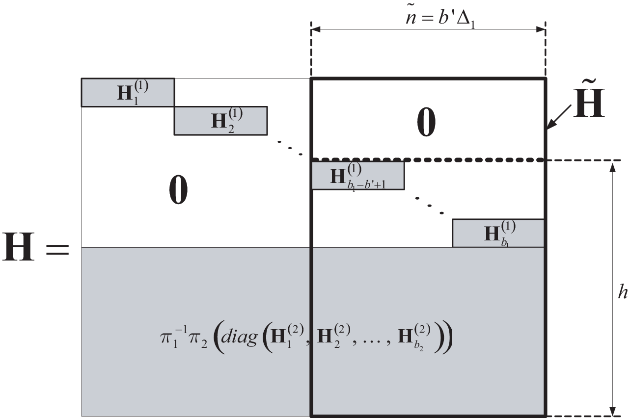
Let us consider a code C~\widetilde{C} of length n~=b′​Δ1\widetilde{n}=b^{\prime}{{\Delta}_{1}}, b′∈ℕb^{\prime}\in\mathbb{N}. The parity-check matrix 𝐇~\widetilde{\bf H} of the code is shown in Fig. 1. The code C~\widetilde{C} correspond to a subcode C′′C^{\prime\prime} of CC. We just need to add a prefix of n−n~n-\widetilde{n} zeros to the word 𝐜~\widetilde{\bf c} of C~\widetilde{C} to obtain the word 𝐜′′{\bf c^{\prime\prime}} of C′′C^{\prime\prime}, i.e.

𝐜′′=(𝟎​𝐜~).{\bf c^{\prime\prime}}=\left(\bf{0}\>\widetilde{\bf c}\right).

Hence,

d⁡(C)≤d⁡(C′′)=d⁡(C~)d\left(C\right)\leq d\left(C^{\prime\prime}\right)=d\left(\widetilde{C}\right)
Refer to caption
Fig. 1: Parity-check matrix of C~\widetilde{C}

Let us consider the code C~\widetilde{C} in more detail. The height hh of its parity-check matrix and hence the number of check symbols in C~\widetilde{C} are upper bounded with (R1−R)​n+b′​(1−R1)​Δ1\left({{R_{1}}-{R}}\right)n+b^{\prime}\left({1-{R_{1}}}\right){\Delta_{1}}, so the dimension k~\widetilde{k} of C~\widetilde{C} can be estimated as follows

k~≥b′​R1​Δ1−(R1−R)​n\widetilde{k}\geq b^{\prime}{R_{1}}{\Delta_{1}}-\left({R_{1}}-{R}\right)n

For the condition k~≥1\widetilde{k}\geq 1 to be satisfied the following condition is sufficient

b′​R1​Δ1−(R1−R)​n≥1b^{\prime}{R_{1}}{\Delta_{1}}-\left({R_{1}}-{R}\right)n\geq 1

So we have such a condition

b′≥R1−RR1​b1+1R1​Δ1b^{\prime}\geq\frac{R_{1}-R}{R_{1}}b_{1}+\frac{1}{R_{1}\Delta_{1}}

After applying the Plotkin bound to C~\widetilde{C} we obtain the needed result

d⁡(C)≤minb′​{qk~−1​(q−1)qk~−1​b′​Δ1},d\left(C\right)\leq\underset{b^{\prime}}{\mathop{\min}}\,\left\{\frac{{{q}^{\widetilde{k}-1}}\left(q-1\right)}{{{q}^{\widetilde{k}}}-1}b^{\prime}{{\Delta}_{1}}\right\},

where b′b^{\prime} satisfy the condition (R1−R)R1​b1+1R1​Δ1≤b′≤b1\frac{\left(R_{1}-R\right)}{{{R}_{1}}}b_{1}+\frac{1}{{{R}_{1}}{{\Delta}_{1}}}\leq b^{\prime}\leq{{b}_{1}}.

∎

Remark 2

In fact we can apply the stronger bound (e.g. the Elias–Bassalygo bound or the MRRW bound) and obtain a tighter bound, but even the Plotkin bound is enough for our purpose.

Now we will derive an asymptotic form of the new bound.

Theorem 2

Let {Ci}i=1∞\left\{{{C}_{i}}\right\}_{i=1}^{\infty} be a sequence of expander codes with rates R⁡(Ci)=RR\left({{C}_{i}}\right)=R and lengths n⁡(Ci)=i×L​C​M⁡(Δ1,Δ2)n\left({{C}_{i}}\right)=i\times\mathop{LCM}\left({{\Delta}_{1}},{{\Delta}_{2}}\right)11 1 by L​C​M​(a,b)LCM(a,b) we mean least common multiplier of aa and bb, i.e. L​C​M​(a,b)=m​i​nm⁡{m:(a|m)∧(b|m)}LCM(a,b)=\mathop{min}\limits_{m}\left\{m:(a|m)\wedge(b|m)\right\} then

δ=limi→∞(d⁡(Ci)n⁡(Ci))≤q−1q​(1−R1+R)\delta=\lim_{i\to\infty}{\left(\frac{d\left({{C}_{i}}\right)}{n\left({{C}_{i}}\right)}\right)}\leq\frac{q-1}{q}\left(\frac{1-R}{1+R}\right)
Proof:

Let us choose

b′=⌈b1​(R1−RR1)⌉+f⁡(n),b^{\prime}=\left\lceil{b_{1}\left({\frac{{R_{1}-R}}{{R_{1}}}}\right)}\right\rceil+f\left(n\right),

where f⁡(n)→∞f\left(n\right)\to\infty while n→∞n\to\infty and f⁡(n)=o⁡(n)f\left(n\right)=o\left(n\right), then

d⁡(C)\displaystyle{d\left(C\right)} ≤\displaystyle{}\leq{} qR1​Δ1​f​(n)−1​(q−1)qR1​Δ1​f​(n)−1\displaystyle\frac{{{q^{{R_{1}}{\Delta_{1}}f\left(n\right)-1}}\left({q-1}\right)}}{{{q^{{R_{1}}{\Delta_{1}}f\left(n\right)}}-1}}
×\displaystyle{\times} ((R1−RR1)​n+(f⁡(n)+1)​Δ1)\displaystyle\>\left({\left({\frac{{R_{1}-R}}{{R_{1}}}}\right)n+\left({f\left(n\right)+1}\right){\Delta_{1}}}\right)

After dividing on nn and taking the limit we have

δ≤q−1q​(R1−RR1).\delta\leq\frac{q-1}{q}\left(\frac{R_{1}-R}{R_{1}}\right). (4)

Finally, from conditions R1≤R2R_{1}\leq R_{2} and (3) we have

R1≤R1+R22≤1+R2R_{1}\leq\frac{R_{1}+R_{2}}{2}\leq\frac{1+R}{2}

and after substituting it to (4) we obtain the needed result

δ≤q−1q​(1−R1+R).\delta\leq\frac{q-1}{q}\left(\frac{1-R}{1+R}\right).

∎

IV Lower bounds

In this section, we obtain the lower bounds on the minimum distance for three code ensembles. Let us introduce needed notations and prove statements common for all the ensembles.

Let ℰ\mathscr{E} be an ensemble of codes of length nn. By A⁡(W)¯{\overline{A\left(W\right)}} we denote a number of code words of weight WW in a code averaged over the ensemble, i.e.

A⁡(W)¯=1|ℰ|​∑i=1|ℰ|Ai​(W),\overline{A\left(W\right)}=\frac{1}{\left|\mathscr{E}\right|}\sum\limits_{i=1}^{\left|\mathscr{E}\right|}{{{A}_{i}}\left(W\right)},

where Ai​(W){{A_{i}}\left(W\right)} is a number of code words of weight WW in a code Ci∈ℰC_{i}\in\mathscr{E}.

Theorem 3

If the condition

∑W=1dA⁡(W)¯<1\sum\limits_{W=1}^{d}{\overline{A\left(W\right)}}<1 (5)

is satisfied for ℰ\mathscr{E} then there exist a code C∈ℰ:d⁡(C)>dC\in\mathscr{E}:d\left(C\right)>d.

Proof:

∑W=1dA⁡(W)¯<1⇒∑W=1d∑i=1|ℰ|Ai​(W)<|ℰ|\sum\limits_{W=1}^{d}{\overline{A\left(W\right)}}<1\Rightarrow\sum\limits_{W=1}^{d}{\sum\limits_{i=1}^{\left|{{\mathscr{E}}}\right|}{{A_{i}}\left(W\right)}}<\left|{{\mathscr{E}}}\right|, which means that the total number of code words of small weight in ℰ\mathscr{E} is less than the number of codes in ℰ\mathscr{E}, therefore there exist a code C∈ℰC\in\mathscr{E} which does not contain the words:

d⁡(C)>dd\left(C\right)>d

∎

Remark 3

Note, that

A⁡(W)¯=1|ℰ|​∑i=1|ℰ|Ai​(W)=1|ℰ|​∑j=1|VW|N⁡(ℰ,𝐯j(W)),\overline{A\left(W\right)}=\frac{1}{{\left|\mathscr{E}\right|}}\sum\limits_{i=1}^{\left|\mathscr{E}\right|}{{A_{i}}\left(W\right)}=\frac{1}{{\left|\mathscr{E}\right|}}\sum\limits_{j=1}^{\left|{{V_{W}}}\right|}{N\left(\mathscr{E},{{\bf{v}}_{j}^{\left(W\right)}}\right)}, (6)

where VW={𝐯(𝐖)∈𝔽qn:‖𝐯(W)‖=W}{{V}_{W}}=\left\{{\bf v^{\left(W\right)}}\in{\mathbb{F}}_{q}^{n}:\left\|{\bf{v}}^{\left(W\right)}\right\|=W\right\} (‖𝐯‖\left\|\bf v\right\| is the Hamming weight of 𝐯\bf v), N⁡(ℰ,𝐯)N\left(\mathscr{E},{{{\bf{v}}}}\right) is a number of codes from ℰ\mathscr{E} containing 𝐯{\bf{v}} as a code word.

Now consider some particular code ensembles.

IV-A Ensemble ℰ1​(Δ0,b)\mathscr{E}_{1}\left({{\Delta_{0}},b}\right) of expander codes with a Reed–Solomon constituent code

Let us consider a block-diagonal matrix

𝐇b=(𝐇0𝟎⋯𝟎𝟎𝐇0⋯𝟎⋮⋱⋱⋮𝟎𝟎⋯𝐇0)(1−R0)​n×n,{{\bf{H}}_{b}}={\left({\begin{array}[]{cccc}{{{\bf{H}}_{0}}}&{\bf{0}}&\cdots&{\bf{0}}\\ {\bf{0}}&{{{\bf{H}}_{0}}}&\cdots&{\bf{0}}\\ \vdots&\ddots&\ddots&\vdots\\ {\bf{0}}&{\bf{0}}&\cdots&{{{\bf{H}}_{0}}}\\ \end{array}}\right)_{\left({1-{R_{0}}}\right)n\times n}}, (7)

where 𝐇0{\bf{H}}_{0} is a parity-check matrix of a (Δ0,R0​Δ0)\left({{\Delta_{0}},{R_{0}}{\Delta_{0}}}\right) Reed–Solomon code over 𝔽q{\mathbb{F}}_{q}, n=Δ0​bn=\Delta_{0}b. By φ⁡(𝐇b){\varphi}\left({{{\bf{H}}_{b}}}\right) we denote the matrix obtained from 𝐇b{\bf{H}}_{b} by an arbitrary permutation of columns and multiplying them by arbitrary nonzero elements of 𝔽q{\mathbb{F}}_{q}. Then the matrix

𝐇=(φ1​(𝐇b)φ2​(𝐇b))2​(1−R0)​n×n{\bf{H}}={\left({\begin{array}[]{c}{{\varphi_{1}}\left({{{\bf{H}}_{b}}}\right)}\\ {{\varphi_{2}}\left({{{\bf{H}}_{b}}}\right)}\\ \end{array}}\right)_{2\left({1-{R_{0}}}\right)n\times n}}

constructed using two matrices as layers, is a sparse parity-check matrix of a code from ℰ1​(Δ0,b)\mathscr{E}_{1}\left({{\Delta_{0}},b}\right).

We define an ensemble ℰ1​(Δ0,b)\mathscr{E}_{1}\left({{\Delta_{0}},b}\right) as follows:

Definition 2

Elements of the ensemble ℰ1​(Δ0,b)\mathscr{E}_{1}\left({{\Delta_{0}},b}\right) are obtained by independent choice of permutations πi{{\pi}_{i}} and nonzero constants ci,j,i=1,2;j=1,2,…,n{{c}_{i,j}},i=1,2;\>j=1,2,\ldots,n, by which parity-check matrices of layers are multiplied.

Remark 4

Each code from ℰ1​(Δ0,b){\mathscr{E}_{1}}\left({{\Delta_{0}},b}\right) is an expander code (Δ1=Δ2=Δ0\Delta_{1}=\Delta_{2}=\Delta_{0}, R1=R2=R0{{R}_{1}}={{R}_{2}}={{R}_{0}}), therefore the upper bound is valid for all of them.

Remark 5

|ℰ1​(Δ0,b)|=(n!​(q−1)n)2\left|\mathscr{E}_{1}\left({{\Delta_{0}},b}\right)\right|={\left({n!{(q-1)^{n}}}\right)^{2}}

Lemma 1

A number of code words of weight WW in a code averaged over the ensemble ℰ1​(Δ0,b)\mathscr{E}_{1}\left({{\Delta_{0}},b}\right)

A⁡(W)¯=(A1​(W))2(q−1)W​(nW),\overline{A\left(W\right)}=\frac{{{{\left({{A_{1}}\left(W\right)}\right)}^{2}}}}{{{{\left({q-1}\right)}^{W}}\left({\begin{array}[]{c}n\\ W\\ \end{array}}\right)}},

where A1​(W){{A}_{1}}\left(W\right) is a number of code words of weight WW in the first layer.

Proof:

Consider a fixed vector 𝐯(W){{\bf{v}}^{\left(W\right)}} of length nn, ‖𝐯(W)‖=W\left\|{{{\bf{v}}^{\left(W\right)}}}\right\|=W. In accordance to equation (6) we need to calculate N⁡(ℰ1,𝐯(W))N\left({\mathscr{E}_{1},{{\bf{v}}^{\left(W\right)}}}\right). Now we consider the ensembles of first (L1L_{1}) and second (L2L_{2}) layers separately. If we know the number of layers from L1L_{1} containing 𝐯(W){{\mathbf{v}}^{\left(W\right)}} as a code word (N⁡(L1,𝐯(W)))\left({N}\left({L_{1},{{\bf{v}}^{\left(W\right)}}}\right)\right) and the number of layers from L2L_{2} containing 𝐯(W){{\mathbf{v}}^{\left(W\right)}} as a code word (N⁡(L2,𝐯(W)))\left({N}\left({L_{2},{{\bf{v}}^{\left(W\right)}}}\right)\right), then

N⁡(ℰ1,𝐯(W))=N⁡(L1,𝐯(W))​N​(L2,𝐯(W)),N\left({\mathscr{E}_{1},{{\bf{v}}^{\left(W\right)}}}\right)={N}\left({L_{1},{{\bf{v}}^{\left(W\right)}}}\right){N}\left({L_{2},{{\bf{v}}^{\left(W\right)}}}\right),

it follows from the fact that permutations and nonzero elements are chosen independently. For the same reason L1=L2L_{1}=L_{2}, hence

N⁡(ℰ1,𝐯(W))=(N⁡(L1,𝐯(W)))2.N\left({\mathscr{E}_{1},{{\bf{v}}^{\left(W\right)}}}\right)={\left({{N}\left({L_{1},{{\bf{v}}^{\left(W\right)}}}\right)}\right)^{2}}. (8)

To calculate N⁡(L1,𝐯(W)){N}\left({L_{1},{{\bf{v}}^{\left(W\right)}}}\right), we proceed as follows: fix a permutation π1\pi_{1}, and perform permutations and multiplications by constants over elements of a vector 𝐯(W){{\bf{v}}^{\left(W\right)}} but not over columns of a parity-check matrix. Clearly, these problems are equivalent, and since nothing depends on a particular permutation π1\pi_{1}, we let it be the identity permutation.

In accordance to properties of φi{{\varphi}_{i}} there are all possible vectors of weight WW among {φi−1​(𝐯(W))}i=1|L1|\left\{{{\varphi}_{i}}^{-1}\left({{\mathbf{v}}^{\left(W\right)}}\right)\right\}_{i=1}^{{\left|L_{1}\right|}} and each of them is repeated KK times, where

K=W!​(n−W)!​(q−1)n−W.K=W!\left(n-W\right)!{{\left(q-1\right)}^{n-W}}.

Thus, we obtain

N⁡(L1,𝐯(W))\displaystyle{N}\left({L_{1},{{\bf{v}}^{\left(W\right)}}}\right) =\displaystyle{}={} A1​(W)​K\displaystyle{{A}_{1}}\left(W\right)K
=\displaystyle{}={} A1​(W)​W!​(n−W)!​(q−1)n−W.\displaystyle{{A}_{1}}\left(W\right)W!\left(n-W\right)!{{\left(q-1\right)}^{n-W}}.

And finally,

N⁡(ℰ1,𝐯(W))=(A1​(W)​W!​(n−W)!​(q−1)n−W)2.N\left({\mathscr{E}_{1},{{\bf{v}}^{\left(W\right)}}}\right)={{\left({{A}_{1}}\left(W\right)W!\left(n-W\right)!{{\left(q-1\right)}^{n-W}}\right)}^{2}}.

One can notice that the value N⁡(ℰ1,𝐯(W))N\left({\mathscr{E}_{1},{{\bf{v}}^{\left(W\right)}}}\right) is the same for all the vectors of weight WW, hence in accordance to (6) we obtain the needed result. ∎

In the next lemma we obtain an upper bound on A⁡(W)¯{\overline{A\left(W\right)}}.

Lemma 2

A number of code words of weight WW in a code averaged over the ensemble ℰ1​(Δ0,b)\mathscr{E}_{1}\left({{\Delta_{0}},b}\right) can be estimated as follows

A⁡(W)¯⩽q−n​F1​(δ,Δ0),\overline{A\left(W\right)}\leqslant{{q}^{-nF_{1}\left(\delta,{{\Delta}_{0}}\right)}},

where

F1​(δ,Δ0)\displaystyle F_{1}\left({\delta,{\Delta_{0}}}\right) =\displaystyle{}={} hq​(δ)+δ​logq⁡(q−1)\displaystyle{h_{q}}\left(\delta\right)+\delta{\log_{q}}\left({q-1}\right)
+\displaystyle{+}  2​maxs>0(δ​logq⁡(s)−1Δ0​logq⁡(g0​(s,Δ0))),\displaystyle\>2\mathop{\max}\limits_{s>0}\left({\delta{{\log}_{q}}\left(s\right)-\frac{1}{{{\Delta_{0}}}}\log_{q}\left({{g_{0}}\left({s,{\Delta_{0}}}\right)}\right)}\right),

δ=Wn\delta=\frac{W}{n}, hq​(δ)=−δ​logq⁡(δ)−(1−δ)​logq⁡(1−δ){{h}_{q}}\left(\delta\right)=-\delta{{\log}_{q}}\left(\delta\right)-\left(1-\delta\right){{\log}_{q}}\left(1-\delta\right) – qq-ry entropy function and g0​(s,Δ0){{g}_{0}}\left(s,{{\Delta}_{0}}\right) is a generating function of weights of code words of constituent code.

Proof:

Note that in each layer the sets of positions occupied by code symbols of constituent codes are disjoint. At the same time, all positions are covered; hence, the generating function of layer G⁡(s)G\left(s\right) looks like:

G⁡(s)=g0nΔ0​(s,Δ0),G\left(s\right)={{g}_{0}}^{\frac{n}{{{\Delta}_{0}}}}\left(s,{{\Delta}_{0}}\right),

then

A1​(W)=[sW]​(g0nΔ0​(s,Δ0)){{A}_{1}}\left(W\right)=\left[{{s}^{W}}\right]\left({{g}_{0}}^{\frac{n}{{{\Delta}_{0}}}}\left(s,{{\Delta}_{0}}\right)\right)

After using an evident estimation

A1​(W)≤mins>0​(g0nΔ0​(s,Δ0)sW){{A}_{1}}\left(W\right)\leq\underset{s>0}{\mathop{\min}}\,\left(\frac{{{g}_{0}}^{\frac{n}{{{\Delta}_{0}}}}\left(s,{{\Delta}_{0}}\right)}{{{s}^{W}}}\right)

we obtain

A⁡(W)¯≤q−n​F1​(δ,Δ0),\overline{A\left(W\right)}\leq{{q}^{-nF_{1}\left(\delta,{{\Delta}_{0}}\right)}},

where δ=Wn\delta=\frac{W}{n}, hq​(δ)=−δ​logq⁡(δ)−(1−δ)​logq⁡(1−δ){{h}_{q}}\left(\delta\right)=-\delta{{\log}_{q}}\left(\delta\right)-\left(1-\delta\right){{\log}_{q}}\left(1-\delta\right),

F1​(δ,Δ0)\displaystyle F_{1}\left({\delta,{\Delta_{0}}}\right) =\displaystyle{}={} hq​(δ)+δ​logq⁡(q−1)\displaystyle{h_{q}}\left(\delta\right)+\delta{\log_{q}}\left({q-1}\right)
+\displaystyle{+}  2​maxs>0(δ​logq⁡(s)−1Δ0​logq⁡(g0​(s,Δ0))).\displaystyle\>2\mathop{\max}\limits_{s>0}\left({\delta{{\log}_{q}}\left(s\right)-\frac{1}{{{\Delta_{0}}}}\log_{q}\left({{g_{0}}\left({s,{\Delta_{0}}}\right)}\right)}\right).

∎

Remark 6

The generating function of weights of code words of a (Δ0,R0​Δ0)\left(\Delta_{0},R_{0}\Delta_{0}\right) Reed–Solomon code can be estimated as follows:

g0​(s,Δ0)≤1+∑i=d0Δ0((Δ0i)​(q−1)i−d0+1​si),{{g}_{0}}\left(s,{{\Delta}_{0}}\right)\leq 1+\sum\limits_{i={d_{0}}}^{{\Delta_{0}}}{\left({\left({\begin{array}[]{c}\Delta_{0}\\ i\\ \end{array}}\right){\left(q-1\right)^{i-{d_{0}}+1}}}s^{i}\right)},

where d0=(1−R0)​Δ0+1d_{0}=\left(1-R_{0}\right)\Delta_{0}+1.

Theorem 4

If there exist at least one positive root (with respect to unknown δ\delta) of equation

F1​(δ,Δ0)=0F_{1}\left({\delta,{\Delta_{0}}}\right)=0 (9)

then in the ensemble ℰ1​(Δ0,b)\mathscr{E}_{1}\left({{\Delta_{0}},b}\right) there exist codes {Ci}i=1N⁡(b)\left\{{{C_{i}}}\right\}_{i=1}^{N(b)} (limb→∞N⁡(b)|ℰ1​(Δ0,b)|=1)\left(\mathop{\lim}\limits_{b\to\infty}{\frac{N(b)}{\left|\mathscr{E}_{1}\left({{\Delta_{0}},b}\right)\right|}}=1\right) such that d⁡(Ci)≥(δ1−ε)​nd\left(C_{i}\right)\geq\left(\delta_{1}-\varepsilon\right)n, where ε\varepsilon is an arbitrary small positive number; δ1\delta_{1} is a positive root of equation (9).

Proof:

We just need to prove that

limn→∞(∑W=1⌊(δ1−ε)​n⌋A⁡(W)¯)=0.\mathop{\lim}\limits_{n\to\infty}\left({\sum\limits_{W=1}^{\left\lfloor{\left({{\delta_{1}}-\varepsilon}\right)n}\right\rfloor}{\overline{A\left(W\right)}}}\right)=0.

The proof is similar to the proof of Theorem 2 in [12]. We omit the proof here. ∎

IV-B Ensemble ℰ2​(Δ0,b)\mathscr{E}_{2}\left({{\Delta_{0}},b}\right) of expander codes with a constituent code from an expurgated ensemble of random codes

In previous section we use a Reed–Solomon code as a constituent code. Unfortunately the length of this code can’t be sufficiently large (Δ0≤q+1\Delta_{0}\leq q+1). In this section we will choose a constituent code from an expurgated ensemble of random codes and use it as a constituent code. In this case we don’t have any constraints on the constituent code length.

Theorem 5

For each Δ0\Delta_{0} and R0R_{0} there exist a linear (Δ0,R0​Δ0)\left(\Delta_{0},R_{0}\Delta_{0}\right) code C0C_{0} with such a spectrum

  1. 1.

    A0​(0)=1A_{0}\left(0\right)=1;

  2. 2.

    A0​(W)≤2​Δ0​(Δ0W)​(q−1)W​q−Δ0​(1−R0)A_{0}\left(W\right)\leq 2\Delta_{0}\left({\begin{array}[]{*{20}{c}}{{\Delta_{0}}}\\ W\\ \end{array}}\right){{\left({q-1}\right)}^{W}}{q^{-{\Delta_{0}}\left({1-{R_{0}}}\right)}}
    for W∈[1,Δ0]W\in\left[1,\Delta_{0}\right].

Proof:

The proof can be found in [13, Ch. 2, Th. 2.4]. ∎

The generating function of weights of code words of C0C_{0} can be estimated as follows:

g0​(s,Δ0)\displaystyle{{g}_{0}}\left(s,{{\Delta}_{0}}\right) ≤\displaystyle{}\leq{} 1\displaystyle 1
+\displaystyle{}+{} ∑i=1Δ0(⌊2​Δ0​(Δ0i)​(q−1)i​q−Δ0​(1−R0)⌋​si),\displaystyle\sum\limits_{i=1}^{{\Delta_{0}}}{\left(\left\lfloor 2\Delta_{0}{\left({\begin{array}[]{c}\Delta_{0}\\ i\\ \end{array}}\right){\left(q-1\right)^{i}}}q^{-\Delta_{0}\left(1-R_{0}\right)}\right\rfloor s^{i}\right)},

All the proofs here are analogical to the proofs for ℰ1​(Δ0,b)\mathscr{E}_{1}\left({{\Delta_{0}},b}\right). We will just give the main result.

Theorem 6

If there exist at least one positive root (with respect to unknown δ\delta) of equation

F2​(δ,Δ0)=0F_{2}\left({\delta,{\Delta_{0}}}\right)=0 (11)

then in the ensemble ℰ2​(Δ0,b)\mathscr{E}_{2}\left({{\Delta_{0}},b}\right) there exist codes {Ci}i=1N⁡(b)\left\{{{C_{i}}}\right\}_{i=1}^{N(b)} (limb→∞N⁡(b)|ℰ2​(Δ0,b)|=1)\left(\mathop{\lim}\limits_{b\to\infty}{\frac{N(b)}{\left|\mathscr{E}_{2}\left({{\Delta_{0}},b}\right)\right|}}=1\right) such that d⁡(Ci)≥(δ2−ε)​nd\left(C_{i}\right)\geq\left(\delta_{2}-\varepsilon\right)n, where ε\varepsilon is an arbitrary small positive number; δ2\delta_{2} is a positive root of equation (11),

F2​(δ,Δ0)\displaystyle F_{2}\left({\delta,{\Delta_{0}}}\right) =\displaystyle{}={} (hq​(δ)+δ​logq⁡(q−1))\displaystyle\left({{h_{q}}\left(\delta\right)+\delta{{\log}_{q}}\left({q-1}\right)}\right)
+\displaystyle+ 2maxs>0⁡(δ​logq⁡(s)−1Δ0​logq⁡(g0​(s,Δ0))).\displaystyle\>\mathop{2{\mathop{\max}}}\limits_{s>0}\left({\delta{{\log}_{q}}\left(s\right)-\frac{1}{{{\Delta_{0}}}}\log_{q}\left({{g_{0}}\left({s,{\Delta_{0}}}\right)}\right)}\right).

IV-C Ensemble ℰ3​(Δ0,b)\mathscr{E}_{3}\left({{\Delta_{0}},b}\right) of non-binary LDPC codes with a Reed–Solomon constituent code

Let us consider the matrix

𝐇=(φ1​(𝐇b)φ2​(𝐇b)⋮φℓ​(𝐇b))ℓ⁡(1−R0)​n×n{\bf{H}}={\left({\begin{array}[]{c}{{\varphi_{1}}\left({{{\bf{H}}_{b}}}\right)}\\ {{\varphi_{2}}\left({{{\bf{H}}_{b}}}\right)}\\ \vdots\\ {{\varphi_{\ell}}\left({{{\bf{H}}_{b}}}\right)}\\ \end{array}}\right)_{\ell\left({1-{R_{0}}}\right)n\times n}}

constructed using ℓ\ell layers, the notion φ⁡(𝐇b){\varphi}\left({{{\bf{H}}_{b}}}\right) was introduced while defining of ℰ1​(Δ0,b)\mathscr{E}_{1}\left({{\Delta_{0}},b}\right) ensemble. The matrix is a sparse parity-check matrix of a code from ℰ3​(Δ0,b)\mathscr{E}_{3}\left({{\Delta_{0}},b}\right).

Definition 3

Elements of the ensemble ℰ3​(Δ0,b)\mathscr{E}_{3}\left({{\Delta_{0}},b}\right) are obtained by independent choice of permutations πi{{\pi}_{i}} and nonzero constants ci,j,i=1,2,…,ℓ;j=1, 2,…,n{{c}_{i,j}},i=1,2,\ldots,\ell;\,j=1,\,2,\ldots,n, by which parity-check matrices of layers are multiplied.

Remark 7

The definition is similar to the definition of ensemble ℰ1​(Δ0,b)\mathscr{E}_{1}\left({{\Delta_{0}},b}\right) but the parity-check matrices here consist of ℓ\ell layers rather than 22 ones.

Remark 8

The codes are not expander codes and hence the upper bound is not valid for them. They are given here for comparison with expander codes.

All the proofs here are analogical to the proofs for ℰ1​(Δ0,b)\mathscr{E}_{1}\left({{\Delta_{0}},b}\right). We will just give the main result.

Theorem 7

If there exist at least one positive root (with respect to unknown δ\delta) of equation

F3​(δ,Δ0)=0F_{3}\left({\delta,{\Delta_{0}}}\right)=0 (12)

then in the ensemble ℰ3​(Δ0,b)\mathscr{E}_{3}\left({{\Delta_{0}},b}\right) there exist codes {Ci}i=1N⁡(b)\left\{{{C_{i}}}\right\}_{i=1}^{N(b)} (limb→∞N⁡(b)|ℰ3​(Δ0,b)|=1)\left(\mathop{\lim}\limits_{b\to\infty}{\frac{N(b)}{\left|\mathscr{E}_{3}\left({{\Delta_{0}},b}\right)\right|}}=1\right) such that d⁡(Ci)≥(δ3−ε)​nd\left(C_{i}\right)\geq\left(\delta_{3}-\varepsilon\right)n, where ε\varepsilon is an arbitrary small positive number; δ3\delta_{3} is a positive root of equation (12),

F3​(δ,Δ0)\displaystyle F_{3}\left({\delta,{\Delta_{0}}}\right) =\displaystyle{}={} (ℓ−1)​(hq​(δ)+δ​logq⁡(q−1))\displaystyle\left({\ell-1}\right)\left({{h_{q}}\left(\delta\right)+\delta{{\log}_{q}}\left({q-1}\right)}\right)
+\displaystyle+ ℓmaxs>0⁡(δ​logq⁡(s)−1Δ0​logq⁡(g0​(s,Δ0))).\displaystyle\>\mathop{\ell{\mathop{\max}}}\limits_{s>0}\left({\delta{{\log}_{q}}\left(s\right)-\frac{1}{{{\Delta_{0}}}}\log_{q}\left({{g_{0}}\left({s,{\Delta_{0}}}\right)}\right)}\right).

V Numerical results

Results obtained for q=64q=64 and q=1024q=1024 are shown in Tables I and II, respectively. The result for ℰ1\mathscr{E}_{1}, ℰ2\mathscr{E}_{2} and ℰ3\mathscr{E}_{3} are maximized over Δ0\Delta_{0}. Note that Δ0≤q+1\Delta_{0}\leq q+1 for ℰ1\mathscr{E}_{1} and ℰ3\mathscr{E}_{3}. The derived upper bound lies below the Varshamov-Gilbert bound when R∈(0.25,0.89)R\in\left(0.25;0.89\right) for q=64q=64. This interval is widening while qq is growing. For q=1024q=1024 we have such an interval (0.05;0.99)\left(0.05;0.99\right).

TABLE I: Results for q=64q=64
R VG Upper δ1​(R);Δ0\delta_{1}\left(R\right);\Delta_{0} δ2​(R);Δ0\delta_{2}\left(R\right);\Delta_{0} δ3​(R);Δ0\delta_{3}\left(R\right);\Delta_{0}
1/8 0.7400 0.7656 0.6905; 64 0.6876; 384 0.7355; 16
1/4 0.5894 0.5906 0.4395; 64 0.4454; 448 0.5860; 12
3/8 0.4608 0.4474 0.2440; 64 0.2545; 512 0.4585; 24
1/2 0.3462 0.3281 0.1180; 64 0.1285; 640 0.3445; 28
5/8 0.2427 0.2272 0.0475; 64 0.0556; 832 0.2415; 40
3/4 0.1492 0.1406 0.0135; 64 0.0187; 1024 0.1480; 52
7/8 0.0665 0.0656 0.0010; 64 0.0030; 448 0.0575; 64
TABLE II: Results for q=1024q=1024
R VG Upper δ1​(R);Δ0\delta_{1}\left(R\right);\Delta_{0} δ2​(R);Δ0\delta_{2}\left(R\right);\Delta_{0} δ3​(R);Δ0\delta_{3}\left(R\right);\Delta_{0}
1/8 0.8036 0.7770 0.6590; 224 0.6319; 192 0.8035; 16
1/4 0.6573 0.5994 0.3350; 248 0.3217; 276 0.6570; 16
3/8 0.5252 0.4541 0.1440; 320 0.1374; 304 0.5250; 24
1/2 0.4028 0.3330 0.0545; 332 0.0524; 384 0.4025; 28
5/8 0.2884 0.2305 0.0180; 352 0.0170; 384 0.2880; 40
3/4 0.1817 0.1427 0.0045; 224 0.0045; 640 0.1810; 60
7/8 0.0835 0.0666 0.0005; 128 0.0005; 768 0.0795; 96

VI Conclusion

A new upper bound on the minimum distance of expander codes is derived. The bound lies below the Varshamov-Gilbert bound while q≥32q\geq 32, hence non-binary expander codes are worse than the best existing non-binary codes. Lower bounds for two ensembles of expander codes are obtained. Both of

the bounds lie much below the upper bound. A lower bound for LDPC codes with a Reed–Solomon constituent code is obtained. The bound is very close to the Varshamov-Gilbert bound and lies above the upper bound for expander codes.

References

  • [1] R. Tanner, “A recursive approach to low complexity codes,” IEEE Trans. Inf. Theory, vol. 27, no. 5, pp. 533 – 547, Sep. 1981.
  • [2] M. Sipser and D. Spielman, “Expander codes,” IEEE Trans. Inf. Theory, vol. 42, no. 6, pp. 1710 –1722, Nov. 1996.
  • [3] A. Lubotzky, R. Phillips, and P. Sarnak, “Ramanujan graphs,” Combinatorica, vol. 8, no. 3, pp. 261–277, 1988.
  • [4] G. A. Margulis, “Explicit group theoretical constructions of combinatorial schemes and their applications to the design of expanders and concentrators,” Probl. Inf. Transm., vol. 24, no. 1, pp. 39–46, 1988.
  • [5] D. Spielman, “Linear-time encodable and decodable error-correcting codes,” IEEE Trans. Inf. Theory, vol. 42, no. 6, pp. 1723 –1731, Nov. 1996.
  • [6] G. Zemor, “On expander codes,” IEEE Trans. Inf. Theory, vol. 47, no. 2, pp. 835 –837, Feb. 2001.
  • [7] V. Skachek and R. Roth, “Generalized minimum distance iterative decoding of expander codes,” in Proc. IEEE Information Theory Workshop (ITW), 2003, pp. 245 – 248.
  • [8] A. Barg and G. Zemor, “Distance properties of expander codes,” IEEE Trans. Inf. Theory, vol. 52, no. 1, pp. 78 – 90, 2006.
  • [9] R. Gallager, Low Density Parity Check Codes. Cambridge, MA: M.I.T. Press, 1963.
  • [10] R. Roth and V. Skachek, “Improved nearly-mds expander codes,” IEEE Trans. Inf. Theory, vol. 52, no. 8, pp. 3650 –3661, 2006.
  • [11] Y. Ben-Haim and S. Litsyn, “Upper bounds on the rate of ldpc codes as a function of minimum distance,” Information Theory, IEEE Transactions on, vol. 52, no. 5, pp. 2092 – 2100, may 2006.
  • [12] A. Frolov and V. Zyablov, “Asymptotic estimation of the fraction of errors correctable by q-ary ldpc codes,” Probl. Inf. Transm., vol. 46, no. 2, pp. 142–159, 2010.
  • [13] E. Blokh and V. Zyablov, Linear Concatenated Codes. Moscow: Nauka, 1963 (In Russian).