Analytical investigation of the phase transition between holographic insulator and superconductor in Gauss-Bonnet gravity

Introducing a new variable $z=r_{s}/r$, we can rewrite Eqs. (8) and (9) into

where the prime here denotes the derivative with respective to $z$.

It has been shown numerically that the solution is unstable and a hair can be developed when the chemical potential is bigger than a critical value, i.e., $\mu>\mu_{c}$. For lower chemical potential, $\mu<\mu_{c}$, the gravitational dual is an AdS soliton with a nonvanishing profile for the scalar field $\psi$, which can be viewed as an insulator phase [10, 18]. Thus, there is a phase transition between the insulator and superconductor phases around the critical chemical potential $\mu_{c}$.

At the critical chemical potential $\mu_{c}$, the scalar field $\psi=0$. So near the critical point Eq. (13) reduces to

With the Neumann-like boundary condition (10) for the gauge field $\phi$ at the tip $r=r_{s}$, we can obtain the physical solution $\phi(z)=\mu$ to Eq. (14) when $\mu<\mu_{c}$. Considering the asymptotic behavior in Eq. (11), close to the critical point this solution indicates that $\rho=0$ near the AdS boundary $z=0$, which gives fairly good agreement with numerical results in Ref. [18].

As $\mu\rightarrow\mu_{c}$, the scalar field equation (12) reduces to

As in [23], we introduce a trial function $F(z)$ near the boundary $z=0$ which satisfies

with $i=+$ or $i=-$. Here we will impose the boundary condition $F(0)=1$ and $F^{\prime}(0)=0$. Then, we can obtain the equation of motion for $F(z)$

Defining a new function

we can rewrite Eq. (17) as

According to the Sturm-Liouville eigenvlaue problem [30], we obtain the expression which can be used to estimate the minimum eigenvalue of $\mu^{2}$

with

In the following calculation, we will assume the trial function to be $F(z)=1-az^{2}$, where $a$ is a constant.

In [18] the condensate $\langle{\cal O}_{+}\rangle$ was numerically calculated in 5-dimensional Gauss-Bonnet AdS soliton background simply by fixing $\psi_{-}=0$. It has been shown numerically that the increase of the Gauss-Bonnet factor $\alpha$ results in the increase of the critical chemical potential, which means that the higher curvature correction will make it harder for the scalar hair to be condensated. Now we can use the S-L method to understand the condensation analytically.

Using Eq. (20) to compute the minimum eigenvalue of $\mu^{2}$ for $i=+$, we can obtain the critical chemical potential $\mu_{c}$ for different strength of the curvature correction and the mass of the scalar field. As an example, we calculate the case of $m^{2}L_{\rm eff}^{2}=0$ in detail. From Eq. (20), we obtain

with

For different values of the Gauss-Bonnet factor, we can get the minimum eigenvalues of $\mu^{2}$ and the corresponding values of $a$, for example, $\mu_{min}^{2}=11.607$ and $a=0.440$ for $\alpha=0.0001$, $\mu_{min}^{2}=12.667$ and $a=0.386$ for $\alpha=0.1$ and $\mu_{min}^{2}=14.365$ and $a=0.257$ for $\alpha=0.2$. Then, we have the critical chemical potential $\mu_{c}=\mu_{min}$ [17]. In Table 1, we present the critical chemical potential $\mu_{c}$ for chosen values of the Gauss-Bonnet coupling $\alpha$ and various masses of the scalar field determined by fixing $m^{2}L_{\rm eff}^{2}$. Comparing with numerical results, we find that the analytic results derived from S-L method are in good agreement with the numerical calculation.

From Table 1, we observe that for the same mass of the scalar field, the critical chemical potential increases when the Gauss-Bonnet factor $\alpha$ becomes bigger. Our analytic result supports the observation obtained numerically that the higher curvature correction can make the scalar hair more difficult to be developed [18, 19, 20, 31, 21, 22, 27, 32, 33, 34, 35, 36]. It is interesting to note that the analytical S-L method can give consistent critical chemical potential with the numerical result even when the mass of the scalar field is zero. This shows that the S-L method is more effective than the matching method. It was realized that the matching method cannot deal with the scalar field with zero mass [18], since for this case the Gauss-Bonnet term does not contribute to the analytic approximation in the matching method [19, 18].

For the same strength of the curvature correction, with the increase of the mass of scalar field, the critical chemical potential $\mu_{c}$ becomes larger. This property also agrees well with the numerical result [18].

In the AdS black hole in Gauss-Bonnet gravity [26], the S-L method was applied by choosing specific mass of the scalar field by fixing $m^{2}L_{eff}^{2}=-3$. For choosing other nonzero values of the mass of scalar field, (4.16) there cannot be integrated analytically so that their (4.17), (4.18) and further steps cannot be derived. In the AdS soliton background, we found a much better situation. (18) above can be integrated analytically when the mass of the scalar field satisfying the Breitenlohner-Freedman bound [37], so that analytically we can observe the condensation with the change of the mass of the scalar field.

If we fix the scalar field mass by choosing values of $m^{2}L^{2}$ instead of $m^{2}L_{\rm eff}^{2}$, the S-L method can give the same qualitative dependence of the critical chemical potential on the Gauss-Bonnet factor as described above when we study the scalar operator $\langle{\cal O}_{+}\rangle$. This supports the numerical computation in the AdS black hole background [19, 18].

Now we concentrate on the scalar operator $\langle{\cal O}_{-}\rangle$ by imposing the condition $\psi_{+}=0$. Fixing the mass of the scalar field by choosing values of $m^{2}L_{\rm eff}^{2}$, the scalar operator $\langle{\cal O}_{-}\rangle$ presents us qualitatively the same behavior of the condensation when we change the strength of the curvature correction as we observed above. With the increase of the Gauss-Bonnet coupling, the critical chemical potential will increase, which shows that the condensation will be harder to develop. But if we fix the mass of the scalar field by choosing values of $m^{2}L^{2}$, analytically we observed completely different condensation behavior as the Gauss-Bonnet coupling changes, see Table 2. Our analytical result got by using S-L method presents the same abnormal behavior as found numerically in [18]. Considering that choosing the mass of the scalar field by selecting the value of $m^{2}L_{\rm eff}^{2}$ contains directly the signature of Gauss-Bonnet factor in the scalar mass, we believe that this way of choosing the scalar field mass can disclose the correct consistent influence due to the Gauss-Bonnet coupling in various condensates.

We will use the S-L method to analytically discuss the critical phenomena for the phase transition between the s-wave holographic insulator and superconductor in the Gauss-Bonnet gravity. We will concentrate on studying the critical exponent for condensation operator and the relations between the charge density and the chemical potential.

The scalar field $\psi$ can be given by Eq. (16) when $\mu\rightarrow\mu_{c}$, so we can rewrite the equations of motion (13) as

Since the condensation for the scalar operator $\langle{\cal O}_{i}\rangle$ is so small, we can expand $\phi(z)$ in small $\langle{\cal O}_{i}\rangle$ as

Considering the boundary condition at the tip, we can get $\chi(1)=0$ and $\chi^{\prime}(1)=constant$. After defining a function

we can obtain the equation of motion for $\chi(z)$

According to the asymptotic behavior in Eq. (11), we can expand $\phi$ when $z\rightarrow 0$ as

From the coefficients of the $z^{0}$ term, we can easily get

If we set

where the function $\xi(z)$ is the solution to the following equation

we will know that

where $\xi(0)=c_{1}-\int_{0}^{1}[c_{2}+\int_{1}^{z}F(x)^{2}x^{2\lambda_{i}-3}dx]\frac{dz}{zf(z)}$ with the integration constants $c_{1}$ and $c_{2}$ determined by the boundary condition $\chi(z)$. For example, fixing $m^{2}L_{\rm eff}^{2}=-15/4$ and $\alpha=0.0001$, we can get $\xi(0)=0.0815$ when $a=0.330$ which results in $\langle{\cal O}_{+}\rangle\approx 1.801(\mu-\mu_{c})^{1/2}$. This agrees well with the result given in [17].

Note that our expression (32) is valid for all cases considered here, thus near the critical point, both of the scalar operators $\langle{\cal O}_{+}\rangle$ and $\langle{\cal O}_{-}\rangle$ satisfy $\langle{\cal O}_{i}\rangle\sim(\mu-\mu_{c})^{1/2}$. This behavior holds for various values of Gauss-Bonnet couplings and masses of the scalar field. The analytic result supports the numerical computation [27, 18] that the phase transition between the s-wave holographic insulator and superconductor belongs to the second order and the critical exponent of the system takes the mean-field value $1/2$. The Gauss-Bonnet coupling will not influence the result.

Considering the coefficients of $z^{1}$ terms in Eq. (28), we find that $\chi^{\prime}(0)\rightarrow 0$ if $z\rightarrow 0$, which is consistent with the following relation by integrating both sides of Eq. (27)

Comparing the coefficients of the $z^{2}$ term in Eq. (28), we can express $\rho$ as

From Eqs. (27) and (33), we arrive at

Using the above formula and Eq. (32), we can deduce

where $\Gamma(\alpha,m)$ is a function of the Gauss-Bonnet coupling and the scalar field mass

Fixing $m^{2}L_{\rm eff}^{2}=-15/4$ and $\alpha=0.0001$, for example, we can get $\Gamma(\alpha,m)=1.330$ when $a=0.330$, so that $\rho=1.330(\mu-\mu_{c})$ for considering the scalar operator $\langle{\cal O}_{+}\rangle$. This is consistent with the result given in [17]. Here we observed that the Gauss-Bonnet coupling will not alter the result. Our analytic finding of a linear relation between the charge density and the chemical potential $\rho\sim(\mu-\mu_{c})$ supports the numerical result reported in [18].

Define the variable $z=r_{s}/r$, the equations of motion (40) and (41) can be expressed in the z coordinate as

where the prime denotes the derivative with respective to $z$.

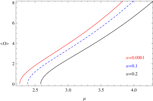
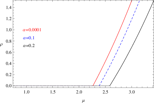
Similar to the analysis in the previous section, if $\mu\leq\mu_{c}$, the field $\psi$ is nearly zero, i.e., $\psi\simeq 0$. Thus, we can obtain the physical solution $\phi(z)=\mu$ to Eq. (44) when $\mu<\mu_{c}$. This is consistent with the numerical results in Fig. 1 which plot the condensates of the operator $\langle{\cal O}\rangle=\psi_{2}$ and charge density $\rho$ with respect to the chemical potential $\mu$ for different Gauss-Bonnet couplings $\alpha$.

As $\mu\rightarrow\mu_{c}$, Eq. (43) will become

We can also define a trial function $F(z)$ near the boundary $z=0$ just as in the last section

with the boundary condition $F(0)=1$ and $F^{\prime}(0)=0$. Therefore, the equation of motion for $F(z)$ is given by

Introducing a new function

we can rewrite Eq. (47) as

Defining the following parameters

we find that, following the Sturm-Liouville eigenvlaue problem [30], the minimum eigenvalue of $\mu^{2}$ can be obtained from variation of the following functional

where we have assumed the trial function to be $F(z)=1-az^{2}$ with a constant $a$.

We can easily obtain the minimum eigenvalues of $\mu^{2}$ and the corresponding values of $a$ for different Gauss-Bonnet couplings $\alpha$, for example, $\mu_{min}^{2}=5.140$ and $a=0.338$ for $\alpha=0.0001$, $\mu_{min}^{2}=5.697$ and $a=0.305$ for $\alpha=0.1$ and $\mu_{min}^{2}=6.691$ and $a=0.223$ for $\alpha=0.2$. Thus, we get the critical chemical potential $\mu_{c}=\mu_{min}$ [17] which has been shown in Table 3 for fixed value of the Gauss-Bonnet factor $\alpha$. In order to compare with numerical results, we also give the critical chemical potential obtained by using the shooting method. Obviously, the agreement of the analytic results derived from S-L method with the numerical calculation is quite impressive.

From Table 3, we also find that the critical chemical potential increases when the Gauss-Bonnet factor $\alpha$ becomes bigger, which shows that the higher order curvature corrections in general make the condensation harder to form, just as observed for the s-wave holographic insulator and superconductor model. This property agrees well with the numerical result shown in Fig. 1.

With Eq. (46), when $\mu\rightarrow\mu_{c}$ the equation of motion (44) can be rewrited as

Note that the condensation value of $\psi(z)$ is so small, we will expand $\phi(z)$ in small $\langle{\cal O}\rangle$ as

with the boundary condition $\chi(1)=0$ at the tip. Using the function defined in Eq. (26), we can get the equation of motion for $\chi(z)$

Near $z\rightarrow 0$, we can also expand $\phi$ as

Comparing the coefficients of the $z^{0}$ term in both sides of the above formula, we can obtain

Considering the following equation for $\xi(z)$

with

we will have

where $\xi(0)=c_{1}-\int_{0}^{1}[c_{2}+\int_{1}^{z}F(x)^{2}x^{3}dx]\frac{dz}{zf(z)}$ with the integration constants $c_{1}$ and $c_{2}$ determined by the boundary condition $\chi(z)$. For example, for the case of $\alpha=0.0001$, we can get $\xi(0)=0.0673$ when $a=0.338$ which results in $\langle{\cal O}\rangle\approx 2.560(\mu-\mu_{c})^{1/2}$. This is in good agreement with the result given in [17, 16].

It should be noted that the relation (59) is valid for all cases considered here, so the condensation $\langle{\cal O}\rangle\sim(\mu-\mu_{c})^{1/2}$ near the critical point for various values of Gauss-Bonnet couplings, which agrees well the numerical results in Fig. 1 that the phase transition between the p-wave holographic insulator and superconductor belongs to the second order and the critical exponent of the system takes the mean-field value $1/2$.

From the coefficients of the $z^{1}$ term in Eq. (55), we obtain that $\chi^{\prime}(0)\rightarrow 0$ which is consistent with the following relation by making integration of both sides of Eq. (54)

For the coefficients of the $z^{2}$ term in Eq. (55), we have

where $\Gamma(\alpha)$ is only the function of the Gauss-Bonnet couplings which can be given by

For example, we can obtain $\Gamma(\alpha)=1.126$ when $a=0.338$ for $\alpha=0.0001$, i.e., the linear relation $\rho=1.126(\mu-\mu_{c})$, which agrees well with the result given in [17]. Still we notice that the Gauss-Bonnet coupling will not change the result. The analytic finding of a linear relation between the charge density and the chemical potential $\rho\sim(\mu-\mu_{c})$ is consistent with the numerical result presented in Fig. 1.