Applications of -continued fraction transformationsThanks: The second author is partially supported by the NSF grant DMS-0703421
Abstract.
We describe a general method of arithmetic coding of geodesics on the modular surface based on the study of one-dimensional Gauss-like maps associated to a two parameter family of continued fractions introduced in [16]. The finite rectangular structure of the attractors of the natural extension maps and the corresponding “reduction theory” play an essential role. In special cases, when an -expansion admits a so-called “dual”, the coding sequences are obtained by juxtaposition of the boundary expansions of the fixed points, and the set of coding sequences is a countable sofic shift. We also prove that the natural extension maps are Bernoulli shifts and compute the density of the absolutely continuous invariant measure and the measure-theoretic entropy of the one-dimensional map.
Key words and phrases:
Continued fractions, modular surface, geodesic flow, invariant measure2000 Mathematics Subject Classification
Primary 37D40, 37B40; Secondary 11A55, 20H051. Introduction and background
In [16], the authors studied a new two-parameter family of continued fraction transformations. These transformations can be defined using the standard generators , of the modular group and considering given by
| (1.1) |
Under the assumption that the parameters belong to the set
one can introduce corresponding continued fraction algorithms by using the first return map of to the interval . Equivalently, these so called -continued fractions can be defined using a generalized integral part function:
| (1.2) |
where denotes the integer part of and .
A starting point of the theory is the following result [16, Theorem 2.1]: if , then any irrational number can be expressed uniquely as an infinite continued fraction of the form
where , and , i.e. the sequence of partial fractions converges to .
It is possible to construct -continued fraction expansions for rational numbers, too. However, such expansions will terminate after finitely many steps if . If , the expansions of rational numbers will end with a tail of ’s, since .
The above family of continued fraction transformations contains three classical examples: the case , described in [22, 12] gives the “minus” (backward) continued fractions, the case , gives the “closest-integer” continued fractions considered first by Hurwitz in [9], and the case , was presented in [19, 14] in connection with a method of coding symbolically the geodesic flow on the modular surface following Artin’s pioneering work [6] and corresponds to the regular “plus” continued fractions with alternating signs of the digits.
The main object of study in [16] is a two-dimensional realization of the natural extension map of , , , defined by
| (1.3) |
Here is the main result of that paper:
Theorem 1.1 ([16]).
There exists an explicit one-dimensional Lebesgue measure zero, uncountable set that lies on the diagonal boundary of such that:
- (1)
for all the map has an attractor on which is essentially bijective.
- (2)
The set consists of two (or one, in degenerate cases) connected components each having finite rectangular structure, i.e. bounded by non-decreasing step-functions with a finite number of steps.
- (3)
Almost every point of the plane () is mapped to after finitely many iterations of .
An essential role in the argument is played by the forward orbits associated to and : to , the upper orbit (i.e. the orbit of ) and the lower orbit (i.e. the orbit of ), and to , the upper orbit (i.e. the orbit of ) and the lower orbit (i.e. the orbit of ). It was proved in [16] that if , then satisfies the finiteness condition, i.e. for both and , their upper and lower orbits are either eventually periodic, or they satisfy the cycle property, i.e. they meet forming a cycle; more precisely, there exist s.t.
where and are the ends of the cycles. If the products of transformations over the upper and lower sides of the cycle are equal, the cycle property is strong, otherwise, it is weak. In both cases the set of the corresponding values is finite; ends of the cycles belong to the set if and only if they are equal to , i.e. if the cycle is weak. The structure of the attractor is explicitly “computed” from the finite set .
The paper is organized as follows. In Section 2 we give some background information about geodesic flows and their representations as special flows over symbolic dynamical systems, and define the coding map. In Section 3 we describe the reduction procedure for coding geodesics via -continued fractions based on the study of the attractor of the associated natural extension map, define the corresponding cross-section set, and introduce the notion of reduced geodesic. In Section 4 we prove that the first return map to the cross-section corresponds to a shift of the coding sequence (Theorem 4.1) and, as a consequence, show that -continued fractions satisfy the Tail Property, i.e. two -equivalent real numbers have the same tails in their -continued fraction expansions. In Section 5 we introduce a notion of a dual code and show that if an -expansion has a dual -expansion, then the coding sequence of a reduced geodesic is obtained by juxtaposition of the -expansion of its attracting endpoint and the -expansion of , where is its repelling endpoint. We also prove that if the -expansion admits a dual, then the set of admissible coding sequences is a sofic shift (Theorem 5.8). In Section 6 we derive formulas for the density of the absolutely continuous invariant measure and the measure-theoretic entropy of the one-dimensional Gauss-type maps and their natural extensions. We also prove that the natural extension maps are Bernoulli shifts. And finally, in Section 7 we apply results of [16] to obtain explicit formulas for invariant measure for the one-dimensional maps for some regions of the parameter set .
2. Geodesic flow on the modular surface and its representation as a special flow over a symbolic dynamical system
Let be the upper half-plane endowed with the hyperbolic metric, be the standard fundamental region of the modular group , and be the modular surface. Let denote the unit tangent bundle of . We will use the coordinates on , where . The quotient space can be identified with the unit tangent bundle of , , although the structure of the fibered bundle has singularities at the elliptic fixed points (see [11, §3.6] for details). Recall that geodesics in this model are half-circles or vertical half-rays. The geodesic flow on is defined as an -action on the unit tangent bundle which moves a tangent vector along the geodesic defined by this vector with unit speed. The geodesic flow on descents to the geodesic flow on the factor via the canonical projection
| (2.1) |
of the unit tangent bundles. Geodesics on are orbits of the geodesic flow .
A cross-section for the geodesic flow is a subset of the unit tangent bundle visited by (almost) every geodesic infinitely often both in the future and in the past. In other words, every defines an oriented geodesic on which will return to infinitely often. The “ceiling” function giving the time of the first return to is defined as follows: if and is the time of the first return of to , then . The map defined by is called the first return map. Thus can be represented as a special flow on the space
given by the formula with the identification .

Let be a finite or countable alphabet, be the space of all bi-infinite sequences endowed with the Tikhonov (product) topology,
be the left shift map, and be a closed -invariant subset. Then is called a symbolic dynamical system. There are some important classes of such dynamical systems. The space is called the full shift (or the topological Bernoulli shift). If the space is given by a set of simple transition rules which can be described with the help of a matrix consisting of zeros and ones, we say that is a one-step topological Markov chain or simply a topological Markov chain (also called a subshift of finite type). A factor of a topological Markov chain is called a sofic shift. (See [10, §1.9] for the definitions.)
In order to represent the geodesic flow as a special flow over a symbolic dynamical system, one needs to choose an appropriate cross-section and code it, i.e. to find an appropriate symbolic dynamical system and a continuous surjective map (in some cases the actual domain of is except a finite or countable set of excluded sequences) defined such that the diagram
is commutative. We can then talk about coding sequences for geodesics defined up to a shift which corresponds to a return of the geodesic to the cross-section . Notice that usually the coding map is not injective but only finite-to-one (see e.g. [2, §3.2 and §5]).
There are two essentially different methods of coding geodesics on surfaces of constant negative curvature. The geometric code, with respect to a given fundamental region, is obtained by a construction universal for all Fuchsian groups. The second method is specific for the modular group and is of arithmetic nature: it uses continued fraction expansions of the end points of the geodesic at infinity and a so-called reduction theory (see [15, 14] for the three classical cases). Here we will describe a general method of arithmetic coding via -continued fractions that is based on study of the attractor of the associated natural extension map. This approach, coupled with ideas of Bowen and Series [7], may be useful for coding of geodesics on quotients by general Fuchsian groups.
3. The reduction procedure
In what follows we will denote the end points of geodesics on by and , and whenever we refer to such geodesics, we use as their coordinates on ().
The reduction procedure for coding symbolically the geodesic flow on the modular surface via continued fraction expansions was presented for the three classical cases in [14]; for a survey on symbolic dynamics of the geodesic flow see also [15]. Here we describe the reduction procedure for -continued fractions and explain how it can be used for coding purposes.
Let be an arbitrary geodesic on from to (irrational end points), and . We construct the sequence of real pairs () defined by
| (3.1) |
Each geodesic from to is -equivalent to by construction. It is convenient to describe this procedure using the reduction map that combines the appropriate iterate of the map :
given by the formula , where is the first digit in the -expansion of . Notice that .
Definition 3.1.
A geodesic in from to is called -reduced if , where
According to Theorem 1.1, for (almost) every geodesic from to in , the above algorithm produces in finitely many steps an -reduced geodesic -equivalent to , and an application of this algorithm to an -reduced geodesic produces another -reduced geodesic. In other words, there exists a positive integer such that and is bijective (with the exception of some segments of the boundary of and their images).
Let be a reduced geodesic with the repelling point and the attracting point
| (3.2) |
Then, by successive applications of the map , we obtain a sequence of real pairs () (see (3.1) above) such that each geodesic from to is -reduced. Using the bijectivity of the map , we extend the sequence (3.2) to the past to obtain a bi-infinite sequence of integers
| (3.3) |
called the coding sequence of , as follows. There exists an integer and a real pair such that and . Notice that . By uniqueness of the -expansion, we conclude that . Continuing inductively, we define the sequence of integers and the real pairs (), where
by and . We also associate to a bi-infinite sequence of -reduced geodesics
| (3.4) |
where is the geodesic from to .
Remark 3.2.
Notice that all “intermediate” geodesics () obtained from using the map are not -reduced.
Proposition 3.3.
Proof.
By [13, Lemma 1.1], it will be sufficient to check that implies , i.e. the digit must be followed by a negative integer and the digit must be followed by a positive integer. We use the following properties of the set that can be derived from our knowledge of the shape of the set determined in [16, Lemmas 5.6, 5.10, 5.11]. The upper part of is contained in the region
| (3.5) | |||||
The lower part of is contained in the region
| (3.6) | |||||
Recall that for an appropriate integer . Suppose . Then . If , then and , and it takes a negative power of to bring it back to (the lower component of) , i.e. . The case , according to (3.5), can only take place if . In this case, , which is equivalent to , a contradiction. Therefore implies . A similar argument shows that implies . We conclude that the formal minus continued fraction converges. In order to prove that the limit is equal to we use the recursive definition of the digits , to write
and the conclusion follows since the formal minus continued fraction converges. ∎
Let
be the upper-half of the unit circle, and
and
be the images of the two vertical boundary components of the fundamental region under (see Figure 3).
Proposition 3.4.
Every -reduced geodesic either intersects or both curves and .
Proof.
If are such that and , then by properties (3.5) and (3.6) of the set , if , then and or , and hence all -reduced geodesics intersect . For the case we have: if , then either or , i.e. the geodesic intersects ; if , then (3.5) implies that , thus the corresponding geodesic intersects if , and it intersects first and then , if . Similarly, for the case we have: if , then either or , i.e. the geodesic intersects ; if , then (3.6) implies that , therefore the corresponding geodesic intersects if , and it intersects first and then if . ∎
Based on Proposition 3.4 we introduce the notion of the cross-section point. It is either the intersection of a reduced geodesic with , or, if does not intersect , its first intersection with .
Now we can define a map
where is the cross-section point on the geodesic from to , and is the unit vector tangent to at . The map is clearly injective. Composed with the canonical projection introduced in (2.1) we obtain a map
Let . This set can be described as follows: , where consists of the unit vectors based on the circular boundary of the fundamental region pointing inward such that the corresponding geodesic on the upper half-plane is -reduced, consists of the unit vectors based on the right vertical boundary of pointing inward such that either or is -reduced (notice that they cannot both be reduced), and consists of the unit vectors based on the left vertical boundary of pointing inward such that either or is -reduced (see Figure 3). Then a.e. orbit of returns to , i.e. is a cross-section for , and is a parametrization of . The map is injective, as follows from Remark 3.2: only one of the geodesics , , , and can be reduced.

4. Symbolic coding of the geodesic flow via -continued fractions.
If is a geodesic on , we denote by the canonical projection of on . For a given geodesic on that can be reduced in finitely many steps, we can always choose its lift to to be -reduced.
The following theorem provides the basis for coding geodesics on the modular surface using -coding sequences.
Theorem 4.1.
Let be an -reduced geodesic on and its projection to . Then
- (1)
each geodesic segment of between successive returns to the cross-section produces an -reduced geodesic on , and each reduced geodesic -equivalent to is obtained this way;
- (2)
the first return of to the cross-section corresponds to a left shift of the coding sequence of .
Proof.
By lifting a geodesic segment on starting on to , we obtain a segment of a geodesic on that is reduced by the definition of the cross-section . A coding sequence of that connects to ,
is obtained by extending the sequence of digits of to the past as explained in the previous section.
Let us assume that , i.e. . The case can be treated similarly. The geodesic is reduced by Theorem 1.1. Let and be the cross-section points on and , respectively. Then ; it is the intersection point of with the circle . We will show that the geodesic segment of , projected to is the segment between two successive returns to the cross-section . Since is the cross-section point on , the geodesic segment projected to is between two returns to . Recall that a geodesic in consists of countably many oriented geodesic segments between consecutive crossings of the boundary of that are obtained by the canonical projection of to .
If is the intersection of with , there are two possibilities. First, when intersects or does not intersect and exists through it circular boundary, and, second, when does not intersect and exists through it left vertical boundary. In the first case the segments in are represented by the intersection with of the following geodesics in : , either or , and either , or .
Suppose that for some intermediate point , the unit vector tangent to at , is projected to . By tracing the geodesic inside , we see that must be projected to with on the boundary of and directed inward. Then the geodesic through
- (a)
enters through its vertical boundary and exits it also through the vertical boundary,
- (b)
enters through its vertical boundary and exits through its circular boundary, or
- (c)
enters through its circular boundary and exits through its vertical boundary.
The following assertions are implied by the analysis of the attractor . In case (a), is not reduced for since , , hence , i.e. , therefore
In case (b), either the segment exits through the circular boundary of , is reduced, and we reached the point on the cross-section. If the segment intersects the circular boundary of , is not reduced. In case (c), is not reduced.
In the second case the first digit of , . This is because would imply which is impossible. Thus is reduced. In this case the geodesic in consists of the intersection with of a single geodesic that enters through its right vertical and leave it through its left vertical boundary, since is reduced. In all cases the geodesic segment projected to is between two consecutive returns to .
If , by Proposition 3.4, since , . Notice that this implies that and , and is reduced. In this case the geodesic in also consists of the intersection with of a single geodesic that enters through its right vertical and leave it through its left vertical boundary, since is reduced, and hence the geodesic segment projected to is between two consecutive returns to . Continuing this argument by induction in both positive and negative direction, we obtain a bi-infinite sequence of points
where is the cross-section point of the reduced geodesic in the sequence of , that represents the sequence of all successive returns of the geodesic in to the cross-section .
If is a reduced geodesic in , -equivalent to , then both project to the same geodesic on . Therefore, the cross-section point of projects on to a cross-section point of for some . This completes the proof of (1).
Since , . The first digit of the past is evidently , and the remaining digits are the same as for . Thus (2) follows. ∎
The following corollary is immediate.
Corollary 4.2.
If is -equivalent to , and both geodesics can be reduced in finitely many steps, then the coding sequences of and differ by a shift.
It implies a very important property of -continued fractions that escapes a direct proof.
Corollary 4.3.
(The Tail Property) For almost every pair of real numbers that are -equivalent, the “tails” of their -continued fraction expansions coincide.
Remark 4.4.
Thus we can talk about coding sequences of geodesics on . To any geodesic that can be reduced in finitely many steps we associate the coding sequence (3.3) of a reduced geodesic -equivalent to it. Corollary 4.2 implies that this definition does not depend on the choice of a particular representative: sequences for equivalent reduced geodesics differ by a shift.
Let be the closure of the set of admissible sequences and be the left shift map. The coding map is defined by
| (4.1) |
This map is essentially bijective.
The symbolic system is defined on the infinite alphabet . The product topology on is induced by the distance function
where , and .
Proposition 4.5.
The map is continuous.
Proof.
If , then the -expansions of the attracting end points and of the corresponding geodesics given by (3.2) have the same first digits. Hence the first convergents of their -expansions are the same, and using the properties of continued fraction and the rate of convergence of[16, Theorem 2.1] we obtain . Similarly, the first digits in the convergent formal minus continued fraction of and are the same, and hence . Therefore the geodesics are uniformly -close. But the tangent vectors are determined by the intersection of the corresponding geodesic with the unit circle or the curves and . Hence, by making large enough we can make as close to as we wish. ∎
In conclusion, the geodesic flow becomes a special flow over a symbolic dynamical system on the infinite alphabet . The ceiling function on coincides with the time of the first return of the associated geodesic to the cross-section . One can establish an explicit formula for as the function of the end points of the corresponding geodesic , , , following the ideas explained in [8]. If and , then is cohomologous to ; more precisely,
5. Dual codes
We have seen that a coding sequence for a reduced geodesic from to (3.3) is comprised from the sequence of digits in -expansion of and the “past”, an infinite sequence of non-zero integers, each digit of which depends on and . In some special cases the “past” only depends on , and, in fact, it will coincide with the sequence of digits of by using a so-called dual expansion to .
Let be the reflection of the plane about the line .
Definition 5.1.
If coincides with the attractor set for some , then the -expansion is called the dual expansion to . If , then the -expansion is called self-dual.
Example 5.2.
The classical situations of - and -expansions are self-dual. Two more sophisticated examples and , respectively, are shown in Figure 4.


Example 5.3.
The expansions , , satisfy a weak cycle property and have dual expansions that are periodic. A classical example in this series is the Hurwitz case whose dual is (see [9, 14]). Their domains are shown in Figure 5.


The following result gives equivalent characterizations for an expansion to admit a dual.
Proposition 5.4.
The following are equivalent:
- (i)
the -expansion has a dual;
- (ii)
the boundary of the lower part of the set does not have -levels with , and the boundary of the upper part of the set does not have -levels with ;
- (iii)
and do not have the strong cycle property.
Proof.
If the -expansion has a dual -expansion, then the parameters are obtained from the boundary of as follows: the right vertical boundary of the upper part of is the ray , and the left vertical boundary of the lower part of is the ray . Now assume that (ii) does not hold. Then at least one of the parameters has the strong cycle property, and either the left boundary of the upper part of or the right boundary of the lower part of is not a straight line. Assume the former. Then the reflection of with respect to the line is not since the map is not bijective on it: the black rectangle in Figure 6 belongs to it, but its image under , colored in grey, does not. Thus (i)(ii).

Conversely, let the vertical line be the right boundary of the upper part of and the vertical line be the left boundary of the lower part of . Let be the intersection of with the horizontal line at the level , and be the intersection of with the horizontal line at the level . Then and . We also see that , where or if is a segment of the boundary of . Then , which implies . By Lemma 5.6 of [16] and , therefore
| (5.1) |
and
| (5.2) |
We now show that is the attractor for , where
| (5.3) |
For with we have with , so by (5.2), hence , and . For with we have with , so , and . Similarly, for with we have with , so , and . This proves that (ii)(i).
Notice that (ii) and (iii) are equivalent by Theorems 4.2 and 4.5 of [16]. ∎
Remark 5.5.
Notice that if an -expansion has a dual, then . This follows from (5.1) and the fact that the relation of duality is symmetric.
Theorem 5.6.
If an -expansion admits a dual expansion , and is an -reduced geodesic, then its coding sequence
| (5.4) |
is obtained by juxtaposing the -expansion of and the -expansion of . This property is preserved under the left shift of the sequence.
Proof.
We will show that the digits in the -expansion of coincide with the digits of the “past” of (5.4). By (5.3), the following diagram
is commutative. The pair , therefore , and . The first digit of the -expansion of is , so
maps to itself. Then
and . Also , and .
Continuing by induction, one proves that all digits of the “past” of the sequence (5.4) are the digits of the -expansion of .
In order to see what happens under a left shift, we reverse the diagram to obtain:
Since the first digit of -expansion of is ,
maps to itself. Then and . Also
hence . ∎
Remark 5.7.
Under conditions of Theorem 5.6, if projects to a closed geodesic on , then its coding sequence is periodic, and , .
Theorem 5.8.
If an -expansion admits a dual expansion, then the symbolic space is a sofic shift.
Proof.
The “natural” (topological) partition of the set related to the alphabet is , where are labeled by the symbols of the alphabet and are defined by the following condition: . In order to prove that the space is sofic one needs to find a topological Markov chain and a surjective continuous map such that .
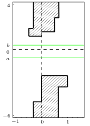
Notice that the elements are rectangles for large ; in fact, at most two elements in the upper part and at most two elements in the lower part of are incomplete rectangles (see Figure 7).

Since has finite rectangular structure, we can sub-divide horizontally these incomplete rectangles into rectangles, and extend the alphabet by adding subscripts to the corresponding elements of . For example, if is subdivided into two rectangles, , the “digit” will give rise to two digits, in the extended alphabet (see Figure 7). We denote the new partition of by . Notice that it consists of rectangles with horizontal and vertical sides. Since the first return to corresponds to the left shift of the coding sequence associated to the geodesic , we see that , where is defined by . Now we define the symbolic space as follows: to each sequence we associate a geodesic by (4.1), and define a new coding sequence , where is defined by , and is the left shift.
We will prove that is a topological Markov chain. For this, in accordance to [2, Theorem 7.9], it is sufficient to prove that for any pair of distinct symbol , and either do not intersect, or intersect “transversally” i.e. their intersection is a rectangle with two horizontal sides belonging to the horizontal boundary of and two vertical sides belonging to the vertical boundary of . Let us recall that (see Remark 5.5). Therefore, if is a complete rectangle, it is, in fact, a square, and its image under is an infinite vertical rectangle intersecting all transversally. If is obtained by subdivision of some and belongs to the lower part of , its horizontal boundaries are the levels of the step-function defining the lower component of , and by Proposition 5.4, since the lower boundary of does not have -levels with , its image is a vertical rectangle intersecting only the lower component of whose horizontal boundaries are the levels of the step-function defining the lower component of . Therefore, all possible intersections with are transversal. A similar argument applies to the case when belongs to the upper part of . The map is obviously continuous, surjective, and, in addition, . ∎
6. Invariant measures and ergodic properties
Based on the finite rectangular geometric structure of the domain and the connections with the geodesic flow on the modular surface, we study some of the measure-theoretic properties of the Gauss-type map ,
| (6.1) |
Notice that the associated natural extension map
| (6.2) |
is obtained from the map induced on the set by the change of coordinates
| (6.3) |
(or, equivalently, on the set by the change of coordinates ). Therefore the domain of is easily identified knowing and may be considered as its “compactification”.
Many of the measure-theoretic properties of and (existence of an absolutely continuous invariant measure, ergodicity) follow from the fact that the geodesic flow on the modular surface can be represented as a special flow on the space
(see Section 2). We recall that and is the ceiling function (the time of the first return to the cross-section ) parametrized by .
We start with the fact that the geodesic flow preserves the smooth (Liouville) measure (see, e.g., [3]), hence preserves the absolutely continuous measure . Using the change of coordinates (6.3), the map preserves the absolutely continuous measure .
The set has finite measure if and , since it is uniformly bounded away from the line (see relations (3.5) and (3.6)). In this situation, we can normalize the measure to obtain the smooth probability measure
| (6.4) |
where . Similarly, if and , the map preserves the smooth probability measure
| (6.5) |
and .
Returning to the Gauss-type map, , one can obtain explicitly a Lebesgue equivalent invariant probability measure by projecting the measure onto the -coordinate (push-forward); this is equivalent to integrating over with respect to the -coordinate as explained in [4].
We can immediately conclude that the systems and are ergodic from the fact that the geodesic flow is ergodic with respect to . By using some well-known results about one dimensional maps that are piecewise monotone and expanding, and the implications for their natural extension maps, we can establish stronger measure-theoretic properties: is exact, and is a Bernoulli shift. Here we follow the presentation from [23] based on [21, 18].
Theorem 6.1.
For any and , the system is exact and its natural extension is a Bernoulli shift.
Proof.
Let us consider first the case . The interval admits a countable partition of open intervals and the map satisfies conditions (A), (F), (U) listed in [23]. Condition (A) is Adler’s distortion estimate:
condition (F) requires the finite image property of the partition ,
while condition (U) is a uniformly expanding condition
Let and be such that and . Consider the open intervals
and
The map satisfies conditions (A), (F), (U) with respect to the partition . Indeed, on , the collection of images consists of four sets , , , , and on . Zweimüller [23] showed that any one-dimensional map for which conditions (A), (F), (U) hold is exact and satisfies Rychlik’s conditions described in [18], hence its natural extension map is Bernoulli.
We analyze now the case . Let be the smallest integer such that . We will show that there exists such that, for every , some iterate with is expanding, i.e. . (For the rest of the proof, we simplify the notations and let denote the map .) Notice that if , then is differentiable at and
Assume that . We look at the following cases:
- (i)
If , then , and .
- (ii)
If , then . Let be such that . Then either there exists such that for and , or for . In the former case we have that
(6.6) while in the latter case
(6.7)
In the case , let be sufficiently small such that
We have:
- (i)
If , then , and . If , then .
- (ii)
In conclusion, there exists a constant such that for every some iterate with satisfies the condition . This implies that the iterate , with , is uniformly expanding, i.e. it satisfies property (U). Since properties (A) and (F) are automatically satisfied by any iterate of (see [23]), we have that is Bernoulli. Using one of Ornstein’s results [17, Theorem 4, p. 39], it follows that is Bernoulli. ∎
The next result gives a formula of the measure theoretic entropy of .
Theorem 6.2.
The measure-theoretic entropy of is given by
| (6.8) |
Proof.
To compute the entropy of this two-dimensional map, we use Abramov’s formula [1]:
where is the normalized Liouville measure . It is well-known that (see [3]) and (see, e.g., [20]). The measure can be represented by the Ambrose-Kakutani theorem [5] as a smooth probability measure on the space
| (6.9) |
where is the probability measure on the cross-section given by (6.4). This implies that
Therefore and
∎
Since is the natural extension of , the measure-theoretic entropies of the two systems coincide, hence
| (6.10) |
As an immediate consequence of the above entropy formula we derive a growth rate relation for the denominators of the partial quotients of -continued fraction expansions, similar to the classical cases.
Proposition 6.3.
Let be the sequence of the denominators of the partial quotients associated to the -continued fraction expansion of . Then
| (6.11) |
Proof.
The proof is similar to the classical case: using the Birkhoff’s ergodic theorem one has
At the same time, Rokhlin’s formula tells us that
hence the conclusion. ∎
7. Some explicit formulas for the invariant measure
In order to obtain explicit formulas for and , one obviously needs an explicit description of the domain . In [16] we describe an algorithmic approach for finding the boundaries of for all parameter pairs outside of a negligible exceptional parameter set . Let us point out that the set may have an arbitrary large number of horizontal boundary segments. The qualitative structure of is given by the cycle properties of and . This structure remains unchanged for all pairs having cycles with similar combinatorial complexity. For a large part of the parameter set the cycle descriptions are relatively simple (see [16, Section 4]) and we discuss it herein.
In what follows, we focus our attention on the situation , and due to the symmetry of the parameter set with respect to the parameter line we assume that .
We treat the case and (for some ). The coordinates of the corners of the boundary segments in the upper region are given by
while the corners of the boundary segments in the lower region are given by
Therefore the set is given by
| (7.1) |

Theorem 7.1.
If and , then
where and with
and
Proof.
The density formulas are obtained from the simple integration result
| (7.2) |
For the density in the upper part of , , all integrals have the lower boundary , hence the result of (7.2) becomes . This gives the description of . For the density in the lower part of , , all integrals have the upper boundary , hence the result and the description of . By a somewhat tedious computation, we get
and this completes the proof. ∎
References
- [1] L. M. Abramov, On the entropy of a flow, Sov. Math. Doklady. 128 (1959), no. 5, 873–875.
- [2] R. Adler, Symbolic dynamics and Markov partitions, Bull. Amer. Math. Soc. 35 (1998), no. 1, 1–56.
- [3] R. Adler, L. Flatto, Cross section maps for geodesic flows, I (The Modular surface), Birkhäuser, Progress in Mathematics (ed. A. Katok) (1982), 103–161.
- [4] R. Adler, L. Flatto, Geodesic flows, interval maps, and symbolic dynamics, Bull. Amer. Math. Soc. 25 (1991), no. 2, 229–334.
- [5] W. Ambrose, S. Kakutani, Structure and continuity of measurable flows, Duke Math. J., 9 (1942), 25–42.
- [6] E. Artin, Ein Mechanisches System mit quasiergodischen Bahnen, Abh. Math. Sem. Univ. Hamburg 3 (1924), 170–175.
- [7] R. Bowen, C. Series, Markov maps associated with Fuchsian groups, Inst. Hautes Études Sci. Publ. Math. No. 50 (1979), 153–170.
- [8] B. Gurevich, S. Katok, Arithmetic coding and entropy for the positive geodesic flow on the modular surface, Moscow Math. J. 1 (2001), no. 4, 569–582.
- [9] A. Hurwitz, Über eine besondere Art der Kettenbruch-Entwicklung reeler Grossen, Acta Math. 12 (1889) 367–405.
- [10] A. Katok, B. Hasselblatt, Introduction to the Modern Theory of Dynamical Systems, Cambridge University Press, 1995.
- [11] S. Katok, Fuchsian Groups, University of Chicago Press, 1992.
- [12] S. Katok, Coding of closed geodesics after Gauss and Morse, Geom. Dedicata 63 (1996), 123–145.
- [13] S. Katok, I. Ugarcovici, Geometrically Markov geodesics on the modular surface, Moscow Math. J. 5 (2005), 135–151.
- [14] S. Katok, I. Ugarcovici, Arithmetic coding of geodesics on the modular surface via continued fractions, 59–77, CWI Tract 135, Math. Centrum, Centrum Wisk. Inform., Amsterdam, 2005.
- [15] S. Katok, I. Ugarcovici, Symbolic dynamics for the modular surface and beyond, Bull. Amer. Math. Soc. 44 (2007), 87–132.
- [16] S. Katok, I. Ugarcovici, Structure of attractors for -continued fraction transformations, Journal of modern Dynamics, 4 (2010), 637–691.
- [17] D. Ornstein, “Ergodic theory, randomness, and dynamical systems”, Yale Univ. Press, New Haven, 1973.
- [18] M. Rychlik, Bounded variation and invariant measures, Studia Math. 76 (1983), 69–80.
- [19] C. Series, On coding geodesics with continued fractions, Enseign. Math. 29 (1980), 67–76.
- [20] D. Sullivan, Entropy, Hausdorff measures old and new, and limit sets of geometrically finite Kleinian groups, Acta Math. 153 (1984), 259–277.
- [21] P. Walters, Invariant measures and equilibrium states for some mappings which expand distances, Trans. Amer. Math. Soc. 236 (1978), 121–153.
- [22] D. Zagier, Zetafunkionen und quadratische Körper: eine Einführung in die höhere Zahlentheorie, Springer-Verlag, 1982.
- [23] R. Zweimüller, Ergodic structure and invariant densities of non-Markovian interval maps with indifferent fixed points, Nonlinearity, 11 (1998), 1263–1276.