Delay Optimal Event Detection on Ad Hoc Wireless Sensor Networks

1 Introduction

A wireless sensor network is formed by tiny, untethered devices (“motes”) that can sense, compute and communicate. Sensor networks have a wide range of applications such as environment monitoring, detecting events, identifying locations of survivors in building and train disasters, and intrusion detection for defense and security applications. For factory and building automation applications, there is increasing interest in replacing wireline sensor networks with wireless sensor networks, due to the potential reduction in costs of engineering, installation, operations, and maintenance [5] [6].

Refer to caption — Figure 1: An ad hoc wireless sensor network with a fusion center is shown. The small circles are the sensor nodes (“motes”), and the lines between them indicate wireless links obtained after a self-organization procedure.

Event detection is an important task in many sensor network applications. In general, an event is associated with a change in the distribution of a related quantity that can be sensed. For example, the event of a gas leakage at any joints in a pipe causes a change in the distribution of pressure at the joint and hence can be detected with the help of pressure sensors. In this paper, we limit our discussion to the centralized fusion model (see Figure 1), in which each mote, in an event detection network, senses and sends some function of its observations (e.g., quantized samples) to the fusion center at a particular rate. The fusion center, by appropriately processing the sequence of values it receives, makes a decision regarding the state of nature, i.e., it decides whether a change has occurred or not.

Our problem is that of minimizing the mean detection delay (the delay between the event occurring and the detection decision at the fusion center) with a bound on the probability of false alarm. We consider a small extent network in which all the sensors have the same coverage, i.e., when the change in distribution occurs it is observed by all the sensors and the statistics of the observations are the same at all the sensors. $N$ sensors synchronously sample their environment at a particular rate. Synchronized operation across sensors is practically possible in networks such as 802.11 WLANs and Zigbee networks since the access point and the PAN coordinator, respectively, transmit beacons that provide all nodes with a time reference. Based on the measurement samples, the nodes send certain values (e.g., quantized samples) to the fusion center. Each value is carried by a packet, which is transmitted using a contention–based multiple access mechanism. Thus, our small extent network problem is a natural extension of the standard change detection problem (see [17] and the references therein) to detection over a random access network. The problem of quickest event detection problem in a large extent network (where the region of interest is much larger than the sensing coverage of any sensor) is considered by us in [11]. Also, a small extent network can be thought of as a cluster in a large extent network and that the decision maker can be thought of as a cluster head.

In this setting, due to the multiple access network delays between the sensor nodes and the fusion center, several possibilities arise. In Figure 2 we show that although the sensors take samples synchronously, due to random access delays the various packets sent by the sensors arrive at the fusion center asynchronously. As shown in the figure, the packets generated due to the samples taken at time $t_{2}$ arrive at the fusion center with a delay of $D^{(1)}_{2},D^{(2)}_{2},D^{(3)}_{2}$ , etc. It can even happen that a packet corresponding to the samples taken at time $t_{3}$ can arrive before one of the packets generated due to the samples taken at time $t_{2}$ .

Figure 3 depicts a general queueing and decision making architecture in the fusion center. All samples are queued in per–node queues in a sequencer. The way the sequencer releases the packets gives rise to the following three cases, the first two of which we study in this paper.

1.

The sequencer queues the samples until all the samples of a “batch” (a batch is the set of samples generated at a sampling instant) are accumulated; it then releases the entire batch to the decision device. The batches arrive to the decision maker in a time sequence order. The decision maker processes the batches without knowledge of the state of the network (i.e., reception times at the fusion center, and the numbers of packets in the various queues). We call this, Network Oblivious Decision Making (NODM). In factory and building automation scenarios, there is a major impetus to replace wireline networks between sensor nodes and controllers. In such applications, the first step could be to retain the fusion algorithm in the controller, while replacing the wireline network with a wireless ad hoc network. Indeed, we show that this approach is optimal for NODM, provided the sampling rate is appropriately optimized.
2.

The sequencer releases samples only in time–sequence order but does not wait for an entire batch to accumulate. The decision maker processes samples as they arrive. We call this, Network Aware Decision Making (NADM). In NADM, whenever the decision maker receives a sample, it has to roll back its decision statistic to the sampling instant, update the decision statistic with the received sample and then update the decision statistic to the current time slot. The decision maker makes a Bayesian update on the decision statistic even if it does not receive a sample in a slot. Thus, NADM requires a modification in the decision making algorithm in the fusion center.
3.

The sequencer does not queue any samples. The fusion center acts on the values from the various sampling instants as they arrive, possibly out of order. The formulation of such a problem would be an interesting topic for future research.

Our Contributions: We find that, in the existing literature on sequential change detection problems (see discussion on related literature below), it has been assumed that, at a sampling instant, the samples from all the sensors reach the fusion center instantaneously. As explained above, however, in our problem the delay in detection is not only due to the detection procedure requiring a certain amount of samples to make a decision (which we call decision delay), but also due to the random packet delay in the multiple access network (which we call network delay). We work with a formulation that accounts for both these delays, while limiting ourselves to the particular fusion center behaviours explained in cases (1) and (2) above.

In Section 2, we discuss the basic change detection problem and setup the model. In Section 3, we formulate the change detection problem over a random access network in a way that naturally includes the network delay. We show that in the case of NODM, the problem objective decouples into a part involving the network delay and a part involving the optimal decision delay, under the condition that the sampling instants are periodic. Then, in Section 4, we consider the special case of a network with a star topology, i.e., all nodes are one hop away from the fusion center and provide a model for contention in the random access network. In Section 5, we formulate the NADM problem where we process the samples as they arrive at the fusion center, but in a time causal manner. The out–of–sequence packets are queued in a sequencing buffer and are released to the decision maker as early as possible. We show in the NADM case that the change–detection problem can be modeled as a Partially Observable Markov Decision Process (POMDP). We show that a sufficient statistic for the observations include the network–state (which include the queue lengths of the sequencing buffer, network–delays) and the posterior probability of change having occurred given the measurements received and the network states. As usual, the optimal policy can be characterised via a Bellman equation, which can then be used to derive insights into the structure of the policy. We show that the optimal policy is a threshold on the posterior probability of change and that the threshold, in general, depends on the network state. Finally, in Section 6 we compare, numerically, the mean detection delay performance of NODM and a simple heuristic algorithm motivated by NADM processing. We show the tradeoff between the sampling rate $r$ and the mean detection delay. Also, we show the tradeoff between the number of sensors and the mean detection delay.

Related Literature: The basic mathematical formulation in this paper is an extension of the classical problem of sequential change detection in a Bayesian framework. The centralized version of this problem was solved by Shiryaev (see [13]). The decentralized version of the problem was introduced by Tenny and Sandell [16]. In the decentralized setting, Veeravalli [17] provided optimal decision rules for the sensors and the fusion center, in the context of conditionally independent sensor observations and a quasi-classical information structure. For a large network setting, Niu and Varshney [9] studied a simple hypothesis testing problem and proposed a counting rule based on the number of alarms. They showed that, for a sufficiently large number of sensors, the detection performance of the counting rule is close to that of the optimal rule. In a recent article on anomaly detection in wireless sensor networks [12], Rajasegarar et al. have provided a survey of statistical and machine learning based techniques for detecting various types of anomalies such as sensor faults, security attacks, and intrusions. In [1] the authors consider the problem of decentralized binary hypothesis testing, where the sensors quantize the observations and the fusion center makes a binary decision between the two hypotheses.

Remark: In the existing literature on the topic of optimal sequential event detection in wireless sensor networks, to the best of our knowledge there has been no prior formulation that incorporates multiple access delay between the sensing nodes and the fusion center. Interestingly, in this paper we introduce, what can be called a cross layer formulation involving sequential decision theory and random access network delays. In particular, we encounter the fork–join queueing model (see, for example, [2]) that arises in distributed computing literature.

2 The Basic Change Detection Problem

In this section, we introduce the model for the basic change detection problem. The notation, we follow, is given here.

$\bullet$

Time is slotted and the slots are indexed by $k=0,1,2\ldots$ . We assume that the length of a slot is unity and that slot $k$ refers to the interval $[k,k+1)$ . Thus, the beginning of slot $k$ indicates the time instant $k$ (see Figure 4).

Figure 5: Change time and the detection instants with and without network delay are shown. The coarse sampling delay is given by $t_{K}-T$ where $t_{K}$ is the first sampling instant after change, and the network delay is given by $U_{\tilde{K}}-t_{\tilde{K}}$ .
$\bullet$

$N$ sensors are synchronously sampling at the rate $r$ samples/slot, i.e., the sensors make an observation every $1/r$ slots and send their observations to the fusion center. Thus, for example, if $r=0.1$ , then a sample is taken by a sensor every $10^{th}$ slot. We assume that $1/r$ is an integer. The sampling instants are denoted $t_{1},t_{2},\ldots$ (see Figure 5). Define $t_{0}=0$ ; note that the first sample is taken at $t_{1}=1/r$ .
$\bullet$

The vector of network delays of the batch $b$ is denoted by

$\mathbf{D}_{b}=\left[D^{(1)}_{b},D^{(2)}_{b},\cdots,D^{(N)}_{b}\right]$

where $D^{(i)}_{b}\in\{1,2,3,\cdots\}$ is the network delay in slots, of the $i$ th component of the $b$ th batch (sampled at $t_{b}=b/r$ ). Also, note that $D_{b}^{(i)}\geqslant 1$ , as it requires one time slot for the transmission of a packet to the fusion center after a successful contention.

\bullet

The state of nature $\Theta\in\{0,1\}$ . $0$ represents the state “before change” and $1$ represents the state “after change”. It is assumed that the change time $T$ (measured in slots), is geometrically distributed i.e.,

	$\displaystyle\mathsf{P}\left(T=0\right)$	$\displaystyle=$	$\displaystyle\rho$
	$\displaystyle\text{and, for}\ k\geqslant 1,\ \ \ \mathsf{P}\left(T=k\mid T>0\right)$	$\displaystyle=$	$\displaystyle p(1-p)^{(k-1)}.$		(1)

The value of $0$ for $T$ accounts for the possibility that the change took place before the observations were made.

$\bullet$

The vector of outputs from the sensor devices at the $b$ th batch is denoted by

$\mathbf{X}_{b}=\left[X^{(1)}_{b},X^{(2)}_{b},\cdots,X^{(N)}_{b}\right]$

where $X^{(i)}_{b}\in\mathcal{X}$ is the $b$ th output at the $i$ th sensor. Given the state of nature, $X^{(i)}_{b}$ are assumed to be (conditionally) independent across sensors and i.i.d. over sampling instants with probability distributions $F_{0}(x)$ and $F_{1}(x)$ before and after the change respectively. $\mathbf{X}_{1}$ corresponds to the first sample taken. In this work, we do not consider the problem of optimal processing of the sensor measurements to yield the sensor outputs, e.g., optimal quantizers (see [17]).
$\bullet$

Let ${S}_{b}$ , $b\geqslant 1$ , be the state of nature at the $b$ th sampling instant and $S_{0}$ the state at time $0$ . Then ${S}_{b}\in\{0,1\}$ , with

$\mathsf{P}\left(S_{0}=1\right)=\rho=1-\mathsf{P}\left(S_{0}=0\right)$

${S}_{b}$ evolves as follows. If ${S}_{b}=0$ for $b\geqslant 0$ , then

$S_{b+1}=\left\{\begin{array}[]{ccc}1&\mbox{w.p.}&p_{r}\\ 0&\mbox{w.p.}&(1-p_{r})\end{array}\right.$

where $p_{r}=1-(1-p)^{1/r}$ . Further, if ${S}_{b}=1$ , then ${S}_{b+1}=1$ . Thus, if ${S}_{0}=0$ , then there is a change from 0 to 1 at the $K$ th sampling instant, where $K$ is geometrically distributed. For $b\geqslant 1$ ,

$\mathsf{P}\left(K=b\right)=p_{r}(1-p_{r})^{b-1}$

Each value to be sent to the fusion center by a node is inserted into a packet which is queued for transmission. It is then transmitted to the fusion center by using a contention based multiple access protocol. A node can directly transmit its observation to the fusion center or route it through other nodes in the system. Each packet takes a time slot to transmit. The MAC protocol and the queues evolve over the same time slots. The fusion center makes a decision about the change depending on whether Network Oblivious (NODM) processing or Network Aware (NADM) processing is employed at the fusion center. In the case of NODM processing, the decision sequence (also called as action sequence), is $A_{u},\ u\geqslant 0$ , with $A_{u}~\in~\{\mathsf{stop~and~declare~change}(1),$ $\mathsf{take~another~sample}(0)\}$ , where $u$ is a time instant at which a complete batch of $N$ samples corresponding to a sampling instant is received by the fusion center. In the case of NADM processing, the decision sequence is $A_{k},\ k\geqslant 0$ , with $A_{k}~\in~\{\mathsf{stop~and~declare~change}(1),$ $\mathsf{take~another~sample}(0)\}$ , i.e., a decision about the change is taken at the beginning of every slot.

3 Network Oblivious Decision Making (NODM)

From Figure 2, we note that although all the components of a batch $b$ are generated at $t_{b}=b/r$ , they reach the fusion center at times $t_{b}+D_{b}^{(i)},i=1,2,\cdots,N$ . In NODM processing, the samples, which are successfully transmitted, are queued in a sequencing buffer as they arrive (see Figure 6) and the sequencer releases a (complete) batch to the decision maker, as soon as all the components of a batch arrive. The decision maker makes a decision about the change at the time instants when a (complete) batch arrives at the fusion center. In the Network Oblivious (NODM) processing, the decision maker is oblivious to the network and processes the batch as though it has just been generated (i.e., as if there is no network, hence the name Network Oblivious Decision Making). We further define (see Figure 5)

$\bullet$

$U_{b},(b\geqslant 1)$ : the random instant at which the fusion center receives the complete batch $\mathbf{X}_{b}$
$\bullet$

$\widetilde{K}\in\{0,1,\dots\}$ : the batch index at which the decision takes place, if there was no network delay. $\widetilde{K}=0$ means that the decision 1 (stop and declare change) is taken before any batch is generated
$\bullet$

$\widetilde{T}=t_{\widetilde{K}}$ : the random time (a sampling instant) at which the fusion center stops and declares change, if there was no network delay
$\bullet$

$\widetilde{U}=U_{\widetilde{K}}$ : the random time slot at which the fusion center stops and declares change, in the presence of network delay
$\bullet$

$D_{b}=U_{b}-t_{b}$ : Sojourn time of the $b$ th batch, i.e., the time taken for all the samples of the $b$ th batch to reach the fusion center. Note that $D_{b}$ is given by $\max\{D_{b}^{(i)}:i=1,2,\cdots,N\}$ . Thus, the delay of the batch $\widetilde{K}$ at which the detector declares a change is $U_{\widetilde{K}}-t_{\widetilde{K}}=\widetilde{U}-\widetilde{T}$

We define the following detection metrics.

Mean Detection Delay

defined as the expected number of slots between the change point $T$ and the stopping time instant $\widetilde{U}$ in the presence of coarse sampling and network delays, i.e., Mean Detection Delay = $\mathsf{E}\!\left[\left(\widetilde{U}-T\right){\bf 1}_{\{\widetilde{T}\geqslant T\}}\right]$ .
Mean Decision Delay

defined as the expected number of slots between the change point $T$ and the stopping time instant $\widetilde{T}$ in the (presence of coarse sampling delay and in the) absence of network delay, i.e., Mean Decision Delay = $\mathsf{E}\!\left[\left(\widetilde{T}-T\right){\bf 1}_{\{\widetilde{T}\geqslant T\}}\right]$ .

With the above model and assumptions, we pose the following NODM problem: Minimize the mean detection delay with a bound on the probability of false alarm, the decision epochs being the time instants when a complete batch of $N$ components corresponding to a sampling instant is received by the fusion center. In Section 5, we pose the problem of making a decision at every slot based on the samples as they arrive at the fusion center. Motivated by the approach in [17] we use the following formulation for a given sampling rate $r$

			$\displaystyle\min\mathsf{E}\!\left[(\widetilde{U}-T){\bf 1}_{\{\widetilde{T}\geqslant T\}}\right]$		(2)
	such that		$\displaystyle\mathsf{P}\left(\widetilde{T}<T\right)\leqslant\alpha$

where $\alpha$ is the constraint on the false alarm probability.

Remark 3.1

Note that if $\alpha\geqslant 1-\rho$ , then the decision making procedure can be stopped and an alarm can be raised even before the first observation. Thus, we assume that $\alpha<1-\rho$ .

Remark 3.2

Note that here we consider $\mathsf{P}\left(\widetilde{T}<T\right)$ as the probability of false alarm and not $\mathsf{P}\left(\widetilde{U}<T\right)$ , i.e., a case as shown in Figure 7 is considered a false alarm. This can be understood as follows: when the decision unit detects a change at slot $\widetilde{U}$ , the measurements that triggered this inference would be carrying the “time stamp” $\widetilde{T}$ , and we infer that the change actually occurred at or before $\widetilde{T}$ . Thus if $\widetilde{T}<T$ , it is an error.

We write the problem defined in Eqn. 2 as

\displaystyle\min_{\Pi_{\alpha}}\mathsf{E}\!\left[(\widetilde{U}-T){\bf 1}_{\{\widetilde{T}\geqslant T\}}\right]

(3)

where $\Pi_{\alpha}$ is the set of detection policies for which $\mathsf{P}\left(\widetilde{T}<T\right)\leqslant\alpha$ .

Theorem 1

If the sampling is periodic at rate $r$ and the batch sojourn time process $D_{b}$ , $b\geqslant 1$ , is stationary with mean $d(r)$ , then

\displaystyle\min_{\Pi_{\alpha}}\mathsf{E}\!\left[(\widetilde{U}-T){\bf 1}_{\{\widetilde{T}\geqslant T\}}\right]

\displaystyle=

\displaystyle(d(r)+l(r))(1-\alpha)-\rho\cdot l(r)+\frac{1}{r}\min_{\Pi_{\alpha}}\mathsf{E}\!\left[\widetilde{K}-K\right]^{+}

where $l(r)$ is the delay due to (coarse) sampling.

Remark 3.3

For example in Figure 5, the delay due to coarse sampling is $t_{2}-T$ , $\widetilde{K}-K=3-2=1$ , and the network delay is $U_{3}-t_{3}$ . The stationarity assumption on $D_{b}$ , $b\geqslant 1$ , is justifiable in a network in which measurements are continuously made, but the detection process is started only at certain times, as needed.

Proof: The following is a sketch of the proof (the details are in the Appendix – I)

	$\displaystyle\min_{\Pi_{\alpha}}\mathsf{E}\!\left[(\widetilde{U}-T){\bf 1}_{\{\widetilde{T}\geqslant T\}}\right]$	$\displaystyle=$	$\displaystyle\min_{\Pi_{\alpha}}\left\{\mathsf{E}\!\left[(\widetilde{U}-\widetilde{T}){\bf 1}_{\{\widetilde{T}\geqslant T\}}\right]+\mathsf{E}\!\left[\widetilde{T}-T\right]^{+}\right\}$
		$\displaystyle=$	$\displaystyle\min_{\Pi_{\alpha}}\left\{\mathsf{E}\!\left[D\right]\left(1-\mathsf{P}\left(\widetilde{T}<T\right)\right)+~\mathsf{E}\!\left[\widetilde{T}-T\right]^{+}\right\}$

where we have used the fact that under periodic sampling, the queueing system evolution and the evolution of the statistical decision problem are independent, i.e., $\widetilde{K}$ is independent of $\{D_{1},D_{2},\ldots\}$ and $\mathsf{E}\!\left[D\right]$ is the mean stationary queueing delay (of a batch). By writing $\mathsf{E}\!\left[D\right]=d(r)$ and using the fact that the problem $\min_{\Pi_{\alpha}}\mathsf{E}\!\left[\widetilde{T}-T\right]^{+}$ is solved by a policy $\pi^{*}_{\alpha}\in\Pi_{\alpha}$ with $\mathsf{P}\left(\widetilde{T}<T\right)=\alpha$ , the problem becomes

\displaystyle d(r)(1-\alpha)+\min_{\Pi_{\alpha}}\mathsf{E}\!\left[\widetilde{T}-T\right]^{+}

\displaystyle=

\displaystyle(d(r)+l(r))(1-\alpha)-\rho\cdot l(r)+\frac{1}{r}\min_{\Pi_{\alpha}}{\mathsf{E}\!\left[\widetilde{K}-K\right]^{+}}

where $l(r)$ is the delay due to sampling. Notice that $\min_{\Pi_{\alpha}}{\mathsf{E}\!\left[\widetilde{K}-K\right]^{+}}$ is the basic change detection problem at the sampling instants.∎

Remark 3.4

It is important to note that the independence between $\widetilde{K}$ and $\{D_{1},D_{2},\ldots\}$ arises from periodic sampling. Actually this is conditional independence given the rate of the periodic sampling process. If, in general, one considers a model in which the sampling is at random times (e.g., the sampling process randomly alternates between periodic sampling at two different rates or if adaptive sampling is used) then we can view it as a time varying sampling rate and the asserted independence will not hold.

We conclude that the problem defined in Eqn. 2 effectively decouples into the sum of the optimal delay in the original optimal detection problem, i.e., $\frac{1}{r}\min_{\Pi_{\alpha}}\mathsf{E}\!\left[\widetilde{K}-K\right]^{+}$ as in [17], a part that captures the network delay, i.e., $d(r)(1-\alpha)$ , and a part that captures the sampling delay, i.e., $l(r)(1-\alpha)-\rho l(r)$ .

4 Network Delay Model

From Theorem 1, it is clear that in NODM processing, the optimal decision device and the queueing system are decoupled. Thus, one can employ an optimal sequential change detection procedure (see [13]) for any random access network (in between the sensor nodes and the fusion center). Also, NODM is oblivious to the random access network (in between the sensor nodes and the fusion center) and processes a received batch as though it has just been generated. In the case of NADM (which we describe in Section 5), the decision maker processes samples, keeping network–delays into account, thus requiring the knowledge of the network dynamics. In this section, we provide a simple model for the random access network, that facilitates the analysis and optimisation of NADM.

$N$ sensors form a star topology¹¹ 1 Note that Theorem 1 is more general and does not assume a star topology. (see Figure 8) ad hoc wireless sensor network with the fusion center as the hub. They synchronously sample their environment at the rate of $r$ samples per slot periodically. At sampling instant $t_{b}=b/r$ , sensor node $i$ generates a packet containing the sample value $X^{(i)}_{b}$ (or some quantized version of it). This packet is then queued first-in-first-out in the buffer behind the radio link. It is as if each sample is a fork operation that puts a packet into each sensor queue (see Figure 6).

The sensor nodes contend for access to the radio channel, and transmit packets when they succeed. The service is modeled as follows. As long as there are packets in any of the queues, successes are assumed to occur at the constant rate of $\sigma~(0<\sigma<1)$ per slot, with the intervals between the successes being i.i.d., geometrically distributed random variables, with mean $1/\sigma$ . If, at the time a success occurs, there are $n$ nodes contending (i.e., $n$ queues are nonempty) then the success is ascribed to any one of the $n$ nodes with equal probability.

The $N$ packets corresponding to a sample arrive at random times at the fusion center. If the fusion center needs to accumulate all the $N$ components of each sample then it must wait for that component of every sample that is the last to depart its mote. This is a join operation (see Figure 6).

It is easily recognized that our service model, in the case of NODM is the discrete time equivalent of generalized processor sharing (GPS – see, for example, [7]), which can be called the FJQ-GPS (fork-join queue (see [2]) with GPS service). In the case of NADM, the service model is just the GPS.

In IEEE 802.11 networks and IEEE 802.15.4 networks, if appropriate parameters are used, then the adaptive backoff mechanism can achieve a throughput that is roughly constant over a wide range of $n$ , the number of contending nodes. This is well known for the CSMA/CA implementation in IEEE 802.11 wireless LANs; see, for example, Figure 9 [8]. For each physical layer rate, the network service rate remains fairly constant with increasing number of nodes. From Figure 10 (taken from [14]) it can be seen that with the default backoff parameters, the saturation throughput of a star topology IEEE 802.15.4 network decreases with the number of nodes $N$ , but with the backoff multiplier $=3$ , the throughput remains almost constant from $N=10$ to $N=50$ [14]; thus, in the latter case our GPS model can be applicable.

Theorem 2

The stationary delay $D$ is a proper random variable with finite mean if and only if $Nr<\sigma$ .

Proof: See Appendix – II.∎

Thus, for the FJQ–GPS queueing system to be stable, the sampling rate $r$ is chosen such that $r<\frac{\sigma}{N}$ .

5 Network Aware Decision Making (NADM)

In Section 3, we formulated the problem of NODM quickest change detection over a random access network, and showed that (when the decision instants are $U_{k}$ , as shown in Figure 5) the optimal decision maker is independent of the random access network, under periodic sampling. Hence, the Shiryaev procedure, which is shown to be delay optimal in the classical change–detection problem (see [13]), can be employed in the decision device independently of the random access network. It is to be noted that the decision maker in the NODM case, waits for a complete batch of $N$ samples to arrive, to make a decision about the change. Thus, the mean detection delay of the NODM has a network–delay component corresponding to a batch of $N$ samples. In this section, we provide an alternative mechanism of fusion at the decision device called Network Aware Decision Making (NADM), in which the fusion algorithm does not wait for an entire batch to arrive, and processes the samples as soon as they arrive, but in a time–causal manner.

We now describe the processing in NADM. Whenever a node (successfully) transmits a sample across the random access network, it is delivered to the decision maker if the decision maker has received all the samples from all the batches generated earlier. Otherwise, the sample is an out–of–sequence sample, and is queued in the sequencing buffer. It follows that, whenever the (successfully) transmitted sample is the last component of the batch that the decision maker is looking for, then the head of line (HOL) components, if any, in the queues of the sequencing buffer are also delivered to the decision maker. This is because, these HOL samples belong to the next batch that the decision maker should process. The decision maker makes a decision about the change at the beginning of every time slot, irrespective of whether it receives a sample or not. In NADM, whenever the decision maker receives a sample, it takes into account the network–delay of the sample while computing the decision statistic. The network–delay is a part of the state of the queueing system which is available to the decision maker. Thus, unlike NODM, the state of the queueing system also plays a role in decision making.

In Section 5.1, we define the state of the queueing system. In Section 5.2, we define the dynamical system whose change of state (from $0$ to $1$ ) is the subject of interest to us. We define the state of the dynamical system as a tuple that contains the queueing state, the state of nature, and a delayed state of nature. The delayed state of nature is included in the state of the system so that the (delayed) sensor–observations that the decision maker receives at time instant $k+1$ depend only on the state, the control, and the noise of the system at time instant $k$ , a property which is desirable to define a sufficient statistic (see page 244, [3]). We explain the evolution of the state of the dynamical system in Section 5.3. In Section 5.4, we formulate the NADM change detection problem and we find a sufficient statistic for the observations in Section 5.5. In Section 5.6, we provide the optimal decision rule for the NADM change detection problem.

5.1 Notation and State of the Queueing System

Recall the notation introduced in Section 2. Time progresses in slots, indexed by $k=0,1,2\cdots$ ; the beginning of slot $k$ is the time instant $k$ . Also, the time instant just after the beginning of time slot is denoted by $k+$ ²² 2 Note that the notation $t+$ denotes a time embedded to the right of $t$ and is different from the notation $(x)^{+}$ . Recall that $(x)^{+}:=\max\{x,0\}$ .. Recall that the nodes take samples at the instants $1/r$ , $2/r$ , $3/r$ , $\cdots$ . We define the state of the queueing system here. Note that the queueing system evolves over slots.

$\bullet$

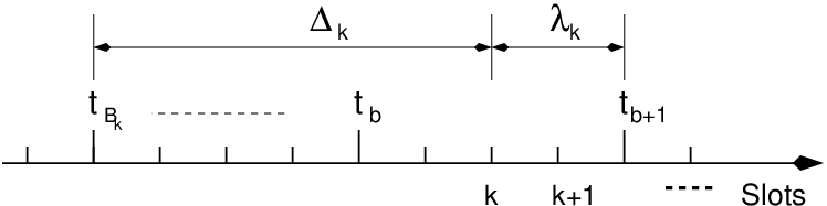
$\lambda_{k}\in\{1,2,\cdots,1/r\}$ denotes the number of time slots to go for the next sampling instant, at the beginning of time slot $k$ (see Figure 11). Thus,

$\displaystyle\lambda_{k}$ $\displaystyle:=$ $\displaystyle\frac{1}{r}-\left(k\mod\frac{1}{r}\right).$ (4)

Thus, $\lambda_{0}=\frac{1}{r},\lambda_{1}=\frac{1}{r}-1,\cdots$ , and at the sampling instants $t_{b}$ , $\lambda_{t_{b}}=\frac{1}{r}$ .

Figure 11: At time $k$ , the decision maker expects samples (or processes samples) from batch $B_{k}$ . Also, at time $k$ , $\lambda_{k}$ is the number of slots to go for the next sampling instant and $\Delta_{k}$ is the number of slots back at which batch $B_{k}$ is generated.
$\bullet$

$B_{k}\in\{1,2,3,\cdots\}$ denotes the index of the batch that is expected to be or is being processed by the decision maker at the beginning of time slot $k$ . Note $B_{0}=B_{1}=\cdots=B_{1/r}=1$ . Also, note that the batch $B_{k}$ is generated at time instant $B_{k}/r$ .

Figure 12: Illustration of a scenario in which $\Delta_{k}=0$ . If the last component from batch $B_{k-1}$ is received at $k$ , and if there is no sampling instant between $t_{B_{k-1}}$ and $k$ , then $\Delta_{k}=0$ . Also, note in this case that $\Delta_{k}=\Delta_{k+1}=\cdots=\Delta_{t_{B_{k}}}=0$ . In this scenario, at time instants $k,k+1,\cdots,t_{B_{k}}$ , all the queues at the sensor nodes and at the sequencer are empty, and at time instant $t_{B_{k}}+$ , all sensor node queues have one packet which is generated at $t_{B_{k}}$ .
$\bullet$

$\Delta_{k}\in\{0,1,2,\cdots\}$ denotes the delay in number of time slots between the time instants $k$ and $B_{k}/r$ (see Figure 11).

$\displaystyle\Delta_{k}$ $\displaystyle:=$ $\displaystyle\max\left\{k-\frac{B_{k}}{r},0\right\}.$ (5)

Note that the batches of samples taken after $B_{k}/r$ and up to (including) $k$ are queued either in the sensor node queues or in the sequencing buffer in the fusion center. If at time $k$ , the fusion center receives a sample which is the last sample from batch $B_{k-1}$ , then $B_{k}=B_{k-1}+1$ . If the sampling instant of the $B_{k}$ th batch is later than $k$ (i.e., $B_{k}/r>k$ ), then $\Delta_{k}=0$ (up to time $B_{k}/r$ at which instant, a new batch is generated). This corresponds to the case, when all the samples generated up to time slot $k$ , have already been processed by the decision maker (see Figure 12). In particular, $\Delta_{0}=\Delta_{1}=\cdots=\Delta_{\frac{1}{r}-1}=0$ .

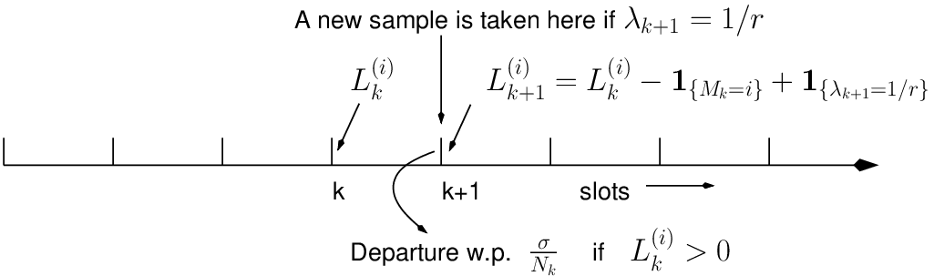
Figure 13: The evolution of $L_{k}^{(i)}$ from time slot $k$ to time slot $k+1$ . If during time slot $k$ , node $i$ transmits (successfully) a packet to the fusion center (i.e., $M_{k}=i$ ), then that packet is flushed out of its queue at the end of time slot $k$ . Also, a new sample is generated (every $1/r$ slots) exactly at the beginning of a time slot. Thus, $L^{(i)}_{k+1}$ , the queue length of sensor node $i$ just after the beginning of time slot $k+1$ (i.e., at $(k+1)+$ ) is given by $L_{k+1}^{(i)}=L_{k}^{(i)}-{\bf 1}_{\{M_{k}=i\}}+{\bf 1}_{\{\lambda_{k+1}=1/r\}}$ .

\bullet

$L_{k}^{(i)}\in\{0,1,2,\cdots\}$ denotes the queue length of the $i$ th sensor node just after the beginning of time slot $k$ (i.e., at time instant $k+$ ). The vector of queue lengths is ${\bf L}_{k}=[L_{k}^{(1)},L_{k}^{(2)},\cdots,L_{k}^{(N)}]$ . Let $N_{k}\in\{0,1,2,\cdots,N\}$ be the number of non–empty queues at the sensor nodes, just after the beginning of time slot $k$ .

N_{k}:=\sum_{i=1}^{N}{\bf 1}_{\{L_{k}^{(i)}>0\}}

i.e., the number of sensor nodes that contend for slot $k$ is $N_{k}$ . Hence, using the network model we have provided in Section 4, the evolution of $L_{k}^{(i)}$ (see Figure 13) is given by the following:

	$\displaystyle L_{0}^{(i)}$	$\displaystyle=$	$\displaystyle 0$
	$\displaystyle L_{k+1}^{(i)}$	$\displaystyle=$	$\displaystyle\left\{\begin{array}[]{lll}L_{k}^{(i)}+{\bf 1}_{\{\lambda_{k+1}=1/r\}}&\ \ \mathrm{w.p.}\ 1&\text{if}\ N_{k}=0,\\ L_{k}^{(i)}+{\bf 1}_{\{\lambda_{k+1}=1/r\}}&\ \ \mathrm{w.p.}\ (1-\sigma)&\text{if}\ N_{k}>0,\\ \max\{L_{k}^{(i)}-1,0\}+{\bf 1}_{\{\lambda_{k+1}=1/r\}}&\ \ \mathrm{w.p.}\ \frac{\sigma}{N_{k}}&\text{if}\ N_{k}>0.\end{array}\right.$

Note that when all the samples generated up to time slot $k$ have already been processed by the decision maker and $k$ is not a sampling instant, i.e., $\Delta_{k}=0$ and $\lambda_{k}\neq 1/r$ , then ${\bf L}_{k}={\bf 0}$ (as there are no outstanding samples in the system). For e.g., ${\bf L}_{1}={\bf L}_{2}=\cdots={\bf L}_{1/r-1}={\bf 0}$ . Also, note that just after sampling instant $t_{b}$ , $L_{t_{b}}^{(i)}\geqslant 1$ .

\bullet

$M_{k}\in\{0,1,2,\cdots,N\}$ denotes the index of the node that successfully transmits in slot $k$ . $M_{k}=0$ means that there is no successful transmission in slot $k$ . Thus, from the network model we have provided in Section 4, we note that

\displaystyle M_{k}

\displaystyle=

\displaystyle\left\{\begin{array}[]{lll}0&\mathrm{w.p.}\ 1&\text{if}\ N_{k}=0\\ 0&\mathrm{w.p.}\ (1-\sigma)&\text{if}\ N_{k}>0\\ j&\mathrm{w.p.}\ \frac{\sigma}{N_{k}}&\text{if}\ L_{k}^{(j)}>0,\ j=1,2,\cdots,N\end{array}\right.

$\bullet$

$W_{k}^{(i)}\in\{0,1,2,\cdots\}$ denotes the queue length of the $i$ th sequencing buffer at time $k$ . The vector of queue lengths is given by ${\bf W}_{k}=[W_{k}^{(1)},W_{k}^{(2)},\cdots,W_{k}^{(N)}]$ . Note that ${\bf W}_{k}={\bf 0}$ if $\Delta_{k}=0$ , i.e., the sequencing buffer is empty if there are no outstanding samples in the system. In particular, ${\bf W}_{0}={\bf W}_{1}=\cdots={\bf W}_{\frac{1}{r}}={\bf 0}$ . The evolution of $W_{k}^{(i)}$ is explained in Figure 14. If a sample from node $i$ of a batch later than $B_{k}$ is successfully transmitted during slot $k$ , then $W_{k+1}^{(i)}=W_{k}^{(i)}+1$ . If a sample from node $j$ of batch $B_{k}$ is successfully transmitted and if it is the last sample to be received from batch $B_{k}$ , then the queue lengths of sequencing buffer are decremented by 1, i.e., $W_{k+1}^{(i)}=\max\{W_{k}^{(i)}-1,0\}$ .
$\bullet$

$R_{k}^{(i)}\in\{0,1\}$ denotes whether the sample $X_{B_{k}}^{(i)}$ has been received and processed by the decision maker at time $k$ . $R_{k}^{(i)}=0$ means that the sample $X_{B_{k}}^{(i)}$ has not yet been received by the decision maker and $R_{k}^{(i)}=1$ means that the sample $X_{B_{k}}^{(i)}$ has been received and processed by the decision maker. The vector of $R_{k}^{(i)}$ s is given by ${\bf R}_{k}=[R_{k}^{(1)},R_{k}^{(2)},\cdots,R_{k}^{(N)}]$ . Note that, if $R_{k}^{(i)}=0$ , ${W}_{k}^{(i)}=0$ , i.e., the $i$ th sequencing buffer is empty if the sample expected by the decision maker has not yet been transmitted. Also note that when $\Delta_{k}=0$ , ${\bf R}_{k}={\bf 0}$ , as the samples from the current batch $B_{k}$ have yet to be generated or have just been generated.

We now relate the queue lengths $L_{k}^{(i)}$ and $W_{k}^{(i)}$ . Note that at the beginning of time slot $k$ , $\left\lfloor\frac{k}{1/r}\right\rfloor$ batches have been generated so far, of which $B_{k}-1$ batches are completely received by the decision maker. In batch $B_{k}$ , $i$ th sample is received by the decision maker if $R_{k}^{(i)}=1$ . Hence, at time $k$ , $B_{k}-1+R_{k}^{(i)}$ samples generated by node $i$ have been processed by the decision maker and the remaining samples are in the sensor and sequencing queues. Thus, we have

$\displaystyle L_{k}^{(i)}+W_{k}^{(i)}$	$\displaystyle=$	$\displaystyle\left\lfloor\frac{k}{1/r}\right\rfloor-\left(B_{k}-1\right)-R_{k}^{(i)}$	(8)
	$\displaystyle=$	$\displaystyle\left\lfloor\frac{k-B_{k}/r+1/r}{1/r}\right\rfloor-R_{k}^{(i)}$
	$\displaystyle=$	$\displaystyle\left\{\begin{array}[]{ll}\left\lfloor\frac{\Delta_{k}}{1/r}\right\rfloor+1-R_{k}^{(i)}&\hskip 31.29802pt\text{if}\ k>B_{k}/r\\ 1-R_{k}^{(i)}&\hskip 31.29802pt\text{if}\ k=B_{k}/r\\ -R_{k}^{(i)}&\hskip 31.29802pt\text{if}\ k<B_{k}/r\end{array}\right.$

Recalling the definition of $\Delta_{k}$ , we write the above Eqn. as,

\displaystyle L_{k}^{(i)}+W_{k}^{(i)}

\displaystyle=

\displaystyle\left\{\begin{array}[]{ll}\left\lfloor\frac{\Delta_{k}}{1/r}\right\rfloor+1-R_{k}^{(i)}&\hskip 31.29802pt\text{if}\ \Delta_{k}>0\\ 1&\hskip 31.29802pt\text{if}\ \Delta_{k}=0,\lambda_{k}=1/r\\ 0&\hskip 31.29802pt\text{if}\ \Delta_{k}=0,\lambda_{k}\neq 1/r.\end{array}\right.

Note that in the above Eqn. $\Delta_{k}=0,\lambda_{k}=1/r$ (or equivalently $k=B_{k}/r$ ), corresponds to the case when the samples of batch $B_{k}$ have just been taken and all the samples from all previous batches have been processed. Thus, in this case $L_{k}^{(i)}=1$ (as $W_{k}^{(i)}=0$ ). In the case of $\Delta_{k}=0,\lambda_{k}\neq 1/r$ (or equivalently $k<B_{k}/r$ ), all the samples from all previous batches have been processed and a new sample from batch $B_{k}$ is not taken yet. Thus, in this case $L_{k}^{(i)}=0$ (and $W_{k}^{(i)}=0$ ). Hence, given ${\bf Q}_{k}=\left[\lambda_{k},B_{k},\Delta_{k},{\bf W}_{k},{\bf R}_{k}\right]$ , the queue lengths $L_{k}^{(i)}$ s can be computed as

	$\displaystyle L_{k}^{(i)}\ =\ \phi_{L^{(i)}}({\bf Q}_{k})$	$\displaystyle:=$	$\displaystyle\left\{\begin{array}[]{ll}\left\lfloor\frac{\Delta_{k}}{1/r}\right\rfloor+1-R_{k}^{(i)}-W_{k}^{(i)}&\hskip 5.69054pt\text{if}\ \Delta_{k}>0\\ 1&\hskip 5.69054pt\text{if}\ \Delta_{k}=0,\lambda_{k}=1/r\\ 0&\hskip 5.69054pt\text{if}\ \Delta_{k}=0,\lambda_{k}\neq 1/r\end{array}\right..$
	$\displaystyle\text{Also},\ N_{k}\ =\ \phi_{N}({\bf Q}_{k})$	$\displaystyle:=$	$\displaystyle\sum_{i=1}^{N}{\bf 1}_{\{\phi_{L^{(i)}}({\bf Q}_{k})>0\}}.$		(21)

Thus, the state of the queueing system at time $k$ , can be expressed as ${\bf Q}_{k}=\left[\lambda_{k},B_{k},\Delta_{k},{\bf W}_{k},{\bf R}_{k}\right]$ . Note that the decision maker can observe the state ${\bf Q}_{k}$ perfectly. The evolution of the queueing system is explained in the next subsection.

5.2 Evolution of the Queueing System

The evolution of the queueing system from time $k$ to time $k+1$ depends only on $M_{k}$ , the success/no–success of contention on the random access channel. Note that the evolution of $\lambda_{k}$ is deterministic and that of $\Delta_{k}$ depends on $B_{k}$ . Hence, to describe the evolution of ${\bf Q}_{k}$ , it is enough to explain the evolution of $B_{k},{\bf W}_{k}$ , and ${\bf R}_{k}$ for various cases of $M_{k}$ . Let ${\bf Y}_{k+1}\in\{\emptyset\}\cup\left(\cup_{n=1}^{N}\mathcal{X}^{n}\right)$ denote the vector of samples received, if any, by the decision maker at the beginning of slot $k+1$ (i.e., the decision maker can receive a vector of $n$ samples where $n$ ranges from 0 to $N$ ).

At the beginning of time slot $k+1$ , the following possibilities arise:

$\bullet$

No successful transmission: This corresponds to the case i) when all the queues are empty at the sensor nodes ( $N_{k}=0$ ), or ii) when some queues are non–empty at the sensor nodes ( $N_{k}>0$ ), either no queue attempts, or there is more than one attempt (resulting in a collision). In either case, $M_{k}=0$ and the decision maker does not receive any sample, i.e., ${\bf Y}_{k+1}=\emptyset$ . In this case, it is clear that $B_{k+1}=B_{k}$ , ${\bf W}_{k+1}={\bf W}_{k}$ , and ${\bf R}_{k+1}={\bf R}_{k}$ .
$\bullet$

Successful transmission of node $j$ ’s sample from a later batch: This corresponds to the case, when the decision maker has already received the $j$ th component of the current batch $B_{k}$ (i.e., $R_{k}^{(j)}=1$ ) and that it has not received some sample, say $i\neq j$ , from the batch $B_{k}$ (i.e., $R_{k}^{(i)}=0$ , for some $i$ ). The received sample (is an out–of–sequence sample and) is queued in the sequencing buffer ( $W_{k+1}^{(j)}=W_{k}^{(j)}+1$ ). Thus, in this case, $M_{k}=j$ and the decision maker does not receive any sample, i.e., ${\bf Y}_{k+1}=\emptyset$ . In this case, it is clear that $B_{k+1}=B_{k}$ , ${\bf W}_{k+1}={\bf W}_{k}+{\bf e}_{j}$ , and ${\bf R}_{k+1}={\bf R}_{k}$ .
$\bullet$

Successful transmission of node $j$ ’s current sample which is not the last component of the batch $B_{k}$ : This corresponds to the case when the decision maker has not received the $j$ th component of the batch $B_{k}$ before time slot $k$ ( $R_{k}^{(j)}=0$ ), and that it has received all the samples that are generated earlier than that of the successful sample. Also, the fusion center is yet to receive some other component of batch $B_{k}$ (i.e., $\sum_{i=1}^{N}R_{k}^{(i)}<N-1$ ). Thus, in this case, $M_{k}=j$ and the decision maker receives the sample ${\bf Y}_{k+1}=X_{B_{k}}^{(j)}$ . In this case, it is clear that $B_{k+1}=B_{k}$ , ${\bf W}_{k+1}={\bf W}_{k}$ , and ${\bf R}_{k+1}={\bf R}_{k}+{\bf e}_{j}$ .
$\bullet$

Successful transmission of node $j$ ’s current sample which is the last component of the batch $B_{k}$ : This corresponds to the case when the decision maker has not received the $j$ th component of the batch $B_{k}$ before time slot $k$ ( $R_{k}^{(j)}=0$ ), and that it has received all the samples that are generated earlier than that of the successful sample. Also, this sample is the last component of batch $B_{k}$ , that is received by the fusion center. (i.e., $\sum_{i=1}^{N}R_{k}^{(i)}=N-1$ ). In this case (along with the received sample), the queues of the sequencing buffer deliver the head of line (HOL) components (which correspond to the batch index $B_{k}+1$ ), if any, to the decision maker and the queues are decremented by one ( $W_{k+1}^{(i)}=\max\{W_{k}^{(i)}-1,0\}$ ). Thus, $M_{k}=j$ and the decision maker receives the vector of samples ${\bf Y}_{k+1}=\left[X_{B_{k}}^{(j)},X_{B_{k}+1}^{(i^{\prime}_{1})},X_{B_{k}+1}^{(i^{\prime}_{2})},\cdots,X_{B_{k}+1}^{(i^{\prime}_{n-1})}\right]$ where $W_{k}^{(i)}>0$ for $i\in\{i^{\prime}_{1},i^{\prime}_{2},\cdots i^{\prime}_{n-1}\}$ , and $W_{k}^{(i)}=0$ for $i\notin\{i^{\prime}_{1},i^{\prime}_{2},\cdots i^{\prime}_{n-1}\}$ . In this case, $B_{k+1}=B_{k}+1$ , ${\bf W}_{k+1}={\bf W}_{k}-{\bf e}_{i_{1}^{\prime}}-{\bf e}_{i_{2}^{\prime}}-\cdots-{\bf e}_{i_{n-1}^{\prime}}$ , and ${\bf R}_{k+1}={\bf e}_{i_{1}^{\prime}}+{\bf e}_{i_{2}^{\prime}}+\cdots+{\bf e}_{i_{n-1}^{\prime}}$ .

Thus, the state of the queueing system at time $k+1$ can be described by

	$\displaystyle{\bf Q}_{k+1}$	$\displaystyle=$	$\displaystyle\phi_{\bf Q}({\bf Q}_{k},M_{k})$
		$\displaystyle:=$	$\displaystyle\left[\phi_{\lambda}({\bf Q}_{k},M_{k}),\phi_{B}({\bf Q}_{k},M_{k}),\phi_{\Delta}({\bf Q}_{k},M_{k}),\phi_{\bf W}({\bf Q}_{k},M_{k}),\phi_{\bf R}({\bf Q}_{k},M_{k})\right].$

In the next subsection, we provide a model of the dynamical system whose state has the state of nature $\Theta_{k}$ as one of its constituents. The quickest detection of change of $\Theta_{k}$ from 0 to 1 (at a random time $T$ ) is the focus of this paper.

5.3 System State Evolution Model

Let $\Theta_{k}\in\{0,1\},k\geqslant 0$ , be the state of nature at the beginning of time slot $k$ . Recall that $T$ is the change point, i.e., for $k<T$ , $\Theta_{k}=0$ and for $k\geqslant T$ , $\Theta_{k}=1$ , and that the distribution of $T$ is given in Eqn. 1. The state $\Theta_{k}$ is observed only through the sensor measurements, but these are delayed. We will formulate the optimal NADM change detection problem as a partially observable Markov decision process (POMDP) with the delayed observations. The approach and the terminology used here is in accordance with the stochastic control framework in [3]. At time $k$ , a sample, if any, that the decision maker receives is generated at time $B_{k}/r<k$ (i.e., samples arrive at the decision maker with a network–delay of $\Delta_{k}=k-\frac{B_{k}}{r}$ slots). To make an inference about $\Theta_{k}$ from the sensor measurements, we must consider the vector of states of nature that corresponds to the time instants $k-\Delta_{k},k-\Delta_{k}+1,\cdots,k$ . We define the vector of states at time $k$ , ${\bf\Theta}_{k}:=[\Theta_{k-\Delta_{k}},\Theta_{k-\Delta_{k}+1},\cdots,\Theta_{k}]$ . Note that the length of the vector depends on the network–delay $\Delta_{k}$ . When $\Delta_{k}>0$ , ${\bf\Theta}_{k}=[\Theta_{\frac{B_{k}}{r}},\Theta_{\frac{B_{k}}{r}+1},\cdots,\Theta_{k}]$ , and when $\Delta_{k}=0$ , ${\bf\Theta}_{k}$ is just [ $\Theta_{k}]$ .

Consider the discrete–time system, which at the beginning of time slot $k$ is described by the state

\displaystyle\Gamma_{k}

\displaystyle=

\displaystyle[{\bf Q}_{k},{\bf\Theta}_{k}],

where we recall that

	$\displaystyle{\bf Q}_{k}$	$\displaystyle=$	$\displaystyle\bigg[\lambda_{k},B_{k},\Delta_{k},{\bf W}_{k},{\bf R}_{k}\bigg],$
	$\displaystyle{\bf\Theta}_{k}$	$\displaystyle=$	$\displaystyle[\Theta_{k-\Delta_{k}},\Theta_{k-\Delta_{k}+1},\cdots,\Theta_{k}].$

Note that $\Gamma_{0}=\left[\left[\frac{1}{r},1,0,{\bf 0}\right],\Theta_{0}\right]$ . At each time slot $k$ , we have the following set of controls $\{0,1\}$ where 0 represents “take another sample”, and 1 represents “stop and declare change”. Thus, at time slot $k$ , when the control chosen is 1, the state $\Gamma_{k+1}$ is given by a terminal absorbing state ${\sf t}$ ; when the control chosen is 0, the state evolution is given by $\Gamma_{k+1}=[{\bf Q}_{k+1},{\bf\Theta}_{k+1}]$ , where

$\displaystyle{\bf Q}_{k+1}$	$\displaystyle=$	$\displaystyle{\bf\phi}_{{\bf Q}}({\bf Q}_{k},M_{k}),$
$\displaystyle{\bf\Theta}_{k+1}$	$\displaystyle=$	$\displaystyle\left\{\begin{array}[]{ll}\left[\Theta_{k}+{\bf 1}_{\{T=k+1\}}\right],&\text{if}\ \Delta_{k+1}=0\\ \left[\Theta_{k-\Delta_{k}},\Theta_{k-\Delta_{k}+1},\cdots,\Theta_{k},\Theta_{k}+{\bf 1}_{\{T=k+1\}}\right],&\text{if}\ \Delta_{k+1}=\Delta_{k}+1\\ \left[\Theta_{k-\Delta_{k}+\frac{1}{r}},\Theta_{k-\Delta_{k}+\frac{1}{r}+1},\cdots,\Theta_{k},\Theta_{k}+{\bf 1}_{\{T=k+1\}}\right],&\text{if}\ \Delta_{k+1}=\Delta_{k}+1-\frac{1}{r}.\end{array}\right.$	(26)
	$\displaystyle=:$	$\displaystyle{\bf\phi}_{\bf\Theta}\left({\bf\Theta}_{k},{\bf Q}_{k},M_{k},{\bf 1}_{\{T=k+1\}}\right)$	(26)

where it is easy to observe that $\Theta_{k}+{\bf 1}_{\{T=k+1\}}=\Theta_{k+1}$ . When $\Delta_{k+1}=\Delta_{k}+1$ , the batch $B_{k}$ is still in service, and hence, in addition to the current state $\Theta_{k+1}=\Theta_{k}+{\bf 1}_{\{T=k+1\}}$ , we need to keep the states $\Theta_{k-\Delta_{k}},\Theta_{k-\Delta_{k}+1},\cdots,\Theta_{k}$ . Also, when $\Delta_{k+1}=\Delta_{k}+1-\frac{1}{r}$ , then the batch index is incremented, and hence, the vector of states that determines the distribution of the observations sampled at or after $B_{k+1}/r$ and before $k+1$ is given by $\left[\Theta_{k-\Delta_{k}+\frac{1}{r}},\Theta_{k-\Delta_{k}+\frac{1}{r}+1},\cdots,\Theta_{k}\right.$ , $\left.\Theta_{k}+{\bf 1}_{\{T=k+1\}}\right]$ .

Define $O_{k}:={\bf 1}_{\{T=k+1\}}$ , and define ${\bf N}_{k}:=[M_{k},O_{k}]$ be the state–noise during time slot $k$ . The distribution of state–noise ${\bf N}_{k}$ given the state of the discrete–time system $\Gamma_{k}$ is given by $\mathsf{P}\left(M_{k}=m,O_{k}=o\big\arrowvert\Gamma_{k}=\left[{\bf q},{\mbox{\boldmath$\theta$}}\right]\right)$ and is the product of the distribution functions, $\mathsf{P}\left(M_{k}=m\big\arrowvert\Gamma_{k}=\left[{\bf q},{\mbox{\boldmath$\theta$}}\right]\right)$ and $\mathsf{P}\left(O_{k}=o\big\arrowvert\Gamma_{k}=\left[{\bf q},{\mbox{\boldmath$\theta$}}\right]\right)$ . These distribution functions are provided in Appendix – III.

The problem is to detect the change in the state $\Theta_{k}$ as early as possible by sequentially observing the samples at the decision maker.

5.4 The NADM Change Detection Problem

We now formulate the NADM change–detection problem in which the observations from the sensor nodes are sent over a random access network to the fusion center and the fusion center processes the samples in the NADM mode.

In Section 5.3, we defined the state $\Gamma_{k}=[{\bf Q}_{k},{\bf\Theta}_{k}]$ on which we formulate the NADM change detection problem as a POMDP. Recall that at the beginning of slot $k$ , the decision maker receives a vector of sensor measurements ${\bf Y}_{k}$ and observes the state ${\bf Q}_{k}$ of the queueing system. Thus, at time $k$ , ${\bf Z}_{k}=[{\bf Q}_{k},{\bf Y}_{k}]$ is the observation of the decision maker about the state of the dynamical system $\Gamma_{k}$ .

Let $A_{k}\in\{0,1\}$ be the control (or action) chosen by the decision maker after having observed ${\bf Z}_{k}$ at $k$ . Recall that $0$ represents “ $\mathsf{take~another~sample}$ ” and $1$ represents the action “ $\mathsf{stop~and~declare~change}$ ”. Let ${\bf I}_{k}=\left[{\bf Z}_{[0:k]},A_{[0:k-1]}\right]$ be the information vector³³ 3 The notation ${\bf Z}_{[k_{1}:k_{2}]}:={\bf Z}_{k_{1}},{\bf Z}_{k_{1}+1},\cdots,{\bf Z}_{k_{2}}$ that is available to the decision maker, at the beginning of time slot $k$ . Let $\tau$ be a stopping time with respect to the sequence of random variables ${\bf I}_{1},{\bf I}_{2},\cdots$ . Note that $A_{k}=0$ for $k<\tau$ and $A_{k}=1$ for $k\geqslant\tau$ . We are interested in obtaining a stopping time $\tau$ (with respect to the sequence ${\bf I}_{1},{\bf I}_{2},\cdots$ ) that minimizes the mean detection delay subject to a constraint on the probability of false alarm.

	$\displaystyle\min$		$\displaystyle\mathsf{E}\!\left[(\tau-T)^{+}\right]$		(27)
	such that		$\displaystyle\mathsf{P}\left(\tau<T\right)\leqslant\alpha$

Note that in the case of NADM, at any time $k$ , a decision about the change is made based on the information ${\bf I}_{k}$ (which includes the batch index we are processing and the delays). Thus, in the case of NADM, false alarm is defined as the event $\{\tau<T\}$ and, hence, $\tau\geqslant T$ is not classified as a false alarm even if it is due to pre–change measurements only. However, in the case of NODM, this is classified as a false alarm as the decision about the change is based on the batches received until time $k$ .

Let $c$ be the cost per unit delay in detection. We are interested in obtaining a stopping time $\tau^{*}$ that minimizes the expected cost (Bayesian risk) given by

$\displaystyle C(c,\tau^{*})$	$\displaystyle=$	$\displaystyle\min_{\tau}\mathsf{E}\!\left[{\bf 1}_{\{\Theta_{\tau}=0\}}+c\cdot(\tau-T)^{+}\right]$	(28)
	$\displaystyle=$	$\displaystyle\min_{\tau}\mathsf{E}\!\left[{\bf 1}_{\{\Theta_{\tau}=0\}}+c\cdot\sum_{k=0}^{\tau-1}{\bf 1}_{\{\Theta_{k}=1\}}\right]$
	$\displaystyle=$	$\displaystyle\min_{\tau}\mathsf{E}\!\left[g_{\tau}(\Gamma_{\tau},A_{\tau})+\sum_{k=0}^{\tau-1}g_{k}(\Gamma_{k},A_{k})\right]$
	$\displaystyle=$	$\displaystyle\min_{\tau}\mathsf{E}\!\left[\sum_{k=0}^{\infty}g_{k}(\Gamma_{k},A_{k})\right]$

where, as defined earlier, $\Gamma_{k}=[{\bf Q}_{k},{\bf\Theta}_{k}]$ . Let ${\mbox{\boldmath$\theta$}}=[\theta_{\delta},\theta_{\delta-1},\cdots,\theta_{1},\theta_{0}]$ . We define for $k\leqslant\tau$

\displaystyle g_{k}([{\bf q},{\mbox{\boldmath$\theta$}}],a)

\displaystyle=

\displaystyle\left\{\begin{array}[]{ll}0,&\text{if}\ \theta_{0}=0,a=0\\ 1,&\text{if}\ \theta_{0}=0,a=1\\ c,&\text{if}\ \theta_{0}=1,a=0\\ 0,&\text{if}\ \theta_{0}=1,a=1\end{array}\right.

and for $k>\tau$ , $g_{k}(\cdot,\cdot):=0$ . Recall that $A_{k}=0$ for $k<\tau$ and $A_{k}=1$ for $k\geqslant\tau$ . Note that $A_{k}$ , the control at time slot $k$ , depends only on ${\bf I}_{k}$ . Thus, every stopping time $\tau$ , corresponds to a policy $\mu=(\mu_{0},\mu_{1},\cdots)$ such that $A_{k}=\mu_{k}({\bf I}_{k})$ , with $A_{k}=0$ for $k<\tau$ and $A_{k}=1$ for $k\geqslant\tau$ . Thus, Eqn. 28 can be written as

$\displaystyle C(c,\tau^{*})$	$\displaystyle=$	$\displaystyle\min_{\mu}\mathsf{E}\!\left[\sum_{k=0}^{\infty}g_{k}(\Gamma_{k},A_{k})\right]$	(34)
	$\displaystyle=$	$\displaystyle\min_{\mu}\sum_{k=0}^{\infty}\mathsf{E}\!\left[g_{k}(\Gamma_{k},A_{k})\right]\ \text{(by monotone convergence theorem)}$
	$\displaystyle=$	$\displaystyle\min_{\mu}\sum_{k=0}^{\infty}\mathsf{E}\!\left[g_{k}(\Gamma_{k},\mu_{k}({\bf I}_{k}))\right]$

Since ${\bf\Theta}_{k}$ is observed only through ${\bf I}_{k}$ , we look at a sufficient statistic for ${\bf I}_{k}$ in the next subsection.

5.5 Sufficient Statistic

In Section 5.2, we have illustrated the evolution of the queueing system ${\bf Q}_{k}$ and we have shown in different scenarios, the vector ${\bf Y}_{k}$ received by the decision maker. Recall from Section 5.2 that

\displaystyle{\bf Y}_{k+1}=

\displaystyle\left\{\begin{array}[]{ll}\emptyset,&\ \text{if}\ M_{k}=0,\\ \emptyset,&\ \text{if}\ M_{k}=j>0,R_{k}^{(j)}=1,\\ Y_{k+1,0},&\ \text{if}\ M_{k}=j>0,R_{k}^{(j)}=0,{{\overset{N}{\underset{i=1}{\sum}}}}R_{k}^{(i)}<N-1\\ \left[Y_{k+1,0},Y_{k+1,1},\cdots,Y_{k+1,n}\right],&\ \text{if}\ M_{k}=j>0,R_{k}^{(j)}=0,{{\overset{N}{\underset{i=1}{\sum}}}}R_{k}^{(i)}=N-1,\\ &\ \ \ {{\overset{N}{\underset{i=1}{\sum}}}}{\bf 1}_{\{W_{k}^{(i)}>0\}}=n.\end{array}\right.

Note that $Y_{k+1,0}$ corresponds to $X_{B_{k}}^{(M_{k})}$ . The last part of the above equation corresponds to the last pending sample of the batch $B_{k}$ arriving at the decision maker at time $k+1$ , with some samples from batch $B_{k}+1$ $(=B_{k+1})$ also being released by the sequencer. In this case, the state of nature at the sampling instant of the batch $B_{k+1}=B_{k}+1$ is $\Theta_{k-\Delta_{k}+1/r}$ . Note that $\Theta_{k-\Delta_{k}+1/r}$ is a component of the vector ${\bf\Theta}_{k}$ as $k-\Delta_{k}+1/r=(B_{k}+1)/r<k$ . Thus, the distribution of $Y_{k+1,0},Y_{k+1,1},\cdots,Y_{k+1,n}$ is given by

	$\displaystyle f_{Y_{k+1,0}}(\cdot)=$	$\displaystyle\left\{\begin{array}[]{ll}f_{0}(\cdot),&\text{if}\ \Theta_{k-\Delta_{k}}=0\\ f_{1}(\cdot),&\text{if}\ \Theta_{k-\Delta_{k}}=1\ \text{and}\end{array}\right.$
	$\displaystyle f_{Y_{k+1,i}}(\cdot)=$	$\displaystyle\left\{\begin{array}[]{ll}f_{0}(\cdot),&\text{if}\ \Theta_{k-\Delta_{k}+1/r}=0\\ f_{1}(\cdot),&\text{if}\ \Theta_{k-\Delta_{k}+1/r}=1\end{array}\right.,\ i=1,2,\cdots,n.$

Thus, at time $k+1$ , the current observation ${\bf Y}_{k+1}$ depends only on the previous state $\Gamma_{k}$ , previous action $A_{k}$ , and the previous noise of the system ${\bf N}_{k}$ . Thus, a sufficient statistic is $\left[\mathsf{P}\left(\Gamma_{k}=\left[{\bf q},{\mbox{\boldmath$\theta$}}\right]\big\arrowvert{\bf I}_{k}\right)\right]_{[{\bf q},{\mbox{\boldmath$\theta$}}]\in\mathcal{S}}$ (see page 244, [3]) where $\mathcal{S}$ is the set of all states of the dynamical system defined in Sec. 5.3. Let ${\bf q}=[\lambda,b,\delta,{\bf w},{\bf r}]$ . Note that

			$\displaystyle\mathsf{P}\left(\Gamma_{k}=\left[{\bf q},{\mbox{\boldmath$\theta$}}\right]\big\arrowvert{\bf I}_{k}\right)$
		$\displaystyle=$	$\displaystyle\mathsf{P}\left(\Gamma_{k}=\left[{\bf q},{\mbox{\boldmath$\theta$}}\right]\big\arrowvert{\bf I}_{k-1},{\bf Q}_{k},{\bf Y}_{k}\right)$
		$\displaystyle=$	$\displaystyle{\bf 1}_{\{{\bf Q}_{k}={\bf q}\}}\cdot\mathsf{P}\left({\bf\Theta}_{k}={\mbox{\boldmath$\theta$}}\big\arrowvert{\bf I}_{k-1},{\bf Q}_{k}={\bf q},{\bf Y}_{k}\right)$
		$\displaystyle=$	$\displaystyle{\bf 1}_{\{{\bf Q}_{k}={\bf q}\}}$
			$\displaystyle\cdot\mathsf{P}\left(\left[\Theta_{k-\delta},\Theta_{k-\delta+1},\cdots,\Theta_{k-1},\Theta_{k}\right]=\left[\theta_{\delta},\theta_{\delta-1},\cdots,\theta_{1},\theta_{0}\right]\big\arrowvert{\bf I}_{k-1},{\bf Q}_{k}={\bf q},{\bf Y}_{k}\right)$
		$\displaystyle=$	$\displaystyle{\bf 1}_{\{{\bf Q}_{k}={\bf q}\}}\cdot\mathsf{P}\left(\Theta_{k-\delta}=\theta_{\delta}\big\arrowvert{\bf I}_{k-1},{\bf Q}_{k}={\bf q},{\bf Y}_{k}\right)$
			$\displaystyle\cdot\prod_{j=1}^{\delta}\mathsf{P}\left(\Theta_{k-\delta+j}=\theta_{\delta-j}\big\arrowvert\Theta_{k-\delta+j^{\prime}}=\theta_{\delta-j^{\prime}},j^{\prime}=0,1,\cdots,j-1,{\bf I}_{k-1},{\bf Q}_{k}={\bf q},{\bf Y}_{k}\right)$

Observe that

			$\displaystyle\mathsf{P}\left(\Theta_{k-\delta+j}=\theta_{\delta-j}\big\arrowvert\Theta_{[k-\delta:k-\delta+j-2]},\Theta_{k-\delta+j-1}=0,{\bf I}_{k-1},{\bf Q}_{k}={\bf q},{\bf Y}_{k}\right)$
		$\displaystyle=$	$\displaystyle\left\{\begin{array}[]{ll}1-p,&\text{if}\ \theta_{\delta-j}=0\\ p,&\text{if}\ \theta_{\delta-j}=1\end{array}\right.$

and

			$\displaystyle\mathsf{P}\left(\Theta_{k-\delta+j}=\theta_{\delta-j}\big\arrowvert\Theta_{[k-\delta:k-\delta+j-2]},\Theta_{k-\delta+j-1}=1,{\bf I}_{k-1},{\bf Q}_{k}={\bf q},{\bf Y}_{k}\right)$
		$\displaystyle=$	$\displaystyle\left\{\begin{array}[]{ll}0,&\text{if}\ \theta_{\delta-j}=0\\ 1,&\text{if}\ \theta_{\delta-j}=1.\end{array}\right.$

This is because given $\Theta_{k-\delta}$ , the events $\{\Theta_{k-\delta+j}=\theta_{\delta-j}\}$ , $\left\{{\bf I}_{k-1},{\bf Q}_{k}={\bf q},{\bf Y}_{k}\right\}$ are conditionally independent. Thus, Eqn. 5.5 can be written as

			$\displaystyle\mathsf{P}\left(\Gamma_{k}=\left[{\bf q},{\mbox{\boldmath$\theta$}}\right]\big\arrowvert{\bf I}_{k}\right)$
		$\displaystyle=$	$\displaystyle\left\{\begin{array}[]{ll}{\bf 1}_{\{{\bf Q}_{k}={\bf q}\}}\cdot\mathsf{P}\left(\Theta_{k-\delta}=1\big\arrowvert{\bf I}_{k-1},{\bf Q}_{k}={\bf q},{\bf Y}_{k}\right),&\text{if}\ {\mbox{\boldmath$\theta$}}={\bf 1}\\ {\bf 1}_{\{{\bf Q}_{k}={\bf q}\}}\cdot\mathsf{P}\left(\Theta_{k-\delta}=0\big\arrowvert{\bf I}_{k-1},{\bf Q}_{k}={\bf q},{\bf Y}_{k}\right)\cdot(1-p)^{\delta-j-1}p,&\text{if}\ {\mbox{\boldmath$\theta$}}=[0,\cdots,0,\underbrace{1}_{\theta_{j}},\cdots,1]\\ {\bf 1}_{\{{\bf Q}_{k}={\bf q}\}}\cdot\mathsf{P}\left(\Theta_{k-\delta}=0\big\arrowvert{\bf I}_{k-1},{\bf Q}_{k}={\bf q},{\bf Y}_{k}\right)\cdot(1-p)^{\delta},&\text{if}\ {\mbox{\boldmath$\theta$}}={\bf 0}\end{array}\right.$

Define $\widetilde{\Theta}_{k}:=\Theta_{k-\Delta_{k}}$ , and define

$\displaystyle\Psi_{k}$	$\displaystyle:=$	$\displaystyle\mathsf{P}\left({\widetilde{\Theta}_{k}}=1\big\arrowvert{\bf I}_{k-1},{\bf Q}_{k}=[\lambda,b,\delta,{\bf w},{\bf r}],{\bf Y}_{k}\right)$
	$\displaystyle=$	$\displaystyle\mathsf{P}\left(\Theta_{k-\delta}=1\big\arrowvert{\bf I}_{k-1},{\bf Q}_{k}=[\lambda,b,\delta,{\bf w},{\bf r}],{\bf Y}_{k}\right)$
$\displaystyle\Pi_{k}$	$\displaystyle:=$	$\displaystyle\mathsf{P}\left({\Theta_{k}}=1\big\arrowvert{\bf I}_{k-1},{\bf Q}_{k}=[\lambda,b,\delta,{\bf w},{\bf r}],{\bf Y}_{k}\right)$
	$\displaystyle=$	$\displaystyle\mathsf{P}\left(T\leqslant k\big\arrowvert{\bf I}_{k-1},{\bf Q}_{k}=[\lambda,b,\delta,{\bf w},{\bf r}],{\bf Y}_{k}\right).$

Thus, Eqn. 5.5 can be written as

			$\displaystyle\mathsf{P}\left(\Gamma_{k}=\left[[\lambda,b,\delta,{\bf w},{\bf r}],{\mbox{\boldmath$\theta$}}\right]\big\arrowvert{\bf I}_{k}\right)$
		$\displaystyle=$	$\displaystyle\left\{\begin{array}[]{ll}{\bf 1}_{\{{\bf Q}_{k}=[\lambda,b,\delta,{\bf w},{\bf r}]\}}\cdot\Psi_{k},&\text{if}\ {\mbox{\boldmath$\theta$}}={\bf 1}\\ {\bf 1}_{\{{\bf Q}_{k}=[\lambda,b,\delta,{\bf w},{\bf r}]\}}\cdot(1-\Psi_{k})\cdot(1-p)^{\delta-j-1}p,&\text{if}\ {\mbox{\boldmath$\theta$}}=[0,\cdots,0,\underbrace{1}_{\theta_{j}},\cdots,1]\\ {\bf 1}_{\{{\bf Q}_{k}=[\lambda,b,\delta,{\bf w},{\bf r}]\}}\cdot(1-\Psi_{k})\cdot(1-p)^{\delta},&\text{if}\ {\mbox{\boldmath$\theta$}}={\bf 0}\end{array}\right.$

We now find a relation between $\Pi_{k}$ and $\Psi_{k}$ in the following Lemma.

Lemma 1

The relation between the conditional probabilities $\Pi_{k}$ and $\Psi_{k}$ is given by

\displaystyle\Pi_{k}

\displaystyle=

\displaystyle\hskip 0.0pt\Psi_{k}+(1-\Psi_{k})\left(1-(1-p)^{\delta}\right)

(48)

Proof.

See Appendix – IV. ∎

From Eqn. 5.5 and Lemma 1, it is clear that a sufficient statistic for ${\bf I}_{k}$ is $\nu_{k}=[{\bf Q}_{k},\Pi_{k}]$ . Also, we show in Appendix – V that $\nu_{k}$ can be computed recursively, i.e., when $A_{k}=0$ , $\nu_{k+1}=\left[{\bf Q}_{k+1},\Pi_{k+1}\right]=\left[{\bf Q}_{k+1},\phi_{\Pi}(\nu_{k},{\bf Z}_{k+1})\right]$ , and when $A_{k}=1$ , $\nu_{k+1}={\sf t}$ , a terminal state. Thus, $\nu_{k}$ can be thought of as entering into a terminating (absorbing) state ${\sf t}$ at $\tau$ (i.e., $\nu_{k}=[{\bf Q}_{k},\Pi_{k}]$ for $k<\tau$ and $\nu_{k}={\sf t}$ for $k\geqslant\tau$ ). Since $\nu_{k}$ is sufficient, for every policy $\mu_{k}$ there corresponds a policy $\widetilde{\mu}_{k}$ such that $\mu_{k}({\bf I}_{k})=\widetilde{\mu}_{k}(\nu_{k})$ (see page 244, [3]).

5.6 Optimal Stopping Time $\tau$

Let $\mathcal{Q}$ be the set of all possible states of the queueing system, ${\bf Q}_{k}$ . Thus the state space of the sufficient statistic is $\mathcal{N}=\left(\mathcal{Q}\times[0,\ 1]\right)\cup\{{\sf t}\}$ . Recall that the action space is $\mathcal{A}=\{0,1\}$ . Define the one–stage cost function $\widetilde{g}:\mathcal{N}\times\mathcal{A}\to\mathbb{R}_{+}$ as follows. Let $\nu\in\mathcal{N}$ be a state of the system and let $a\in\mathcal{A}$ be a control. Then,

\displaystyle\widetilde{g}(\nu,a)

\displaystyle=

\displaystyle\left\{\begin{array}[]{ll}0&\text{if}\ \nu={\sf t}\\ c\cdot\pi&\text{if}\ \nu=[{\bf q},\pi],a=0\\ 1-\pi&\text{if}\ \nu=[{\bf q},\pi],a=1.\end{array}\right.

Note from Eqn. 5.4 for $k\leqslant\tau$ that

$\displaystyle\mathsf{E}\!\left[g_{k}(\Theta_{k},A_{k})\right]$	$\displaystyle=$	$\displaystyle\mathsf{E}\!\left[g_{k}(\Theta_{k},\mu_{k}({\bf I}_{k}))\right]$
	$\displaystyle=$	$\displaystyle\mathsf{E}\!\left[\mathsf{E}\!\left[g_{k}(\Theta_{k},\mu_{k}({\bf I}_{k}))\bigg\arrowvert{\bf I}_{k}\right]\right]$
	$\displaystyle=$	$\displaystyle\mathsf{E}\!\left[\widetilde{g}(\nu_{k},\widetilde{\mu}_{k}(\nu_{k}))\right]$

and for $k>\tau$ ,

	$\displaystyle\mathsf{E}\!\left[g_{k}(\Theta_{k},A_{k})\right]$	$\displaystyle=$	$\displaystyle 0$
		$\displaystyle=$	$\displaystyle\mathsf{E}\!\left[\widetilde{g}({\sf t},\cdot)\right]$

Since, $\{\nu_{k}\}$ is a controlled Markov process, and the one–stage cost function $\widetilde{g}(\cdot,\cdot)$ , the transition probability kernel for $A_{k}=1$ and for $A_{k}=0$ (i.e., $\mathsf{P}\left({\bf Z}_{k+1}\big\arrowvert\nu_{k}\right)$ ), do not depend on time $k$ , and the optimization problem defined in Eqn. 34 is over infinite horizon, it is sufficient to look for an optimal policy in the space of stationary Markov policies (see page 83, [4]). Thus, the optimization problem defined in Eqn. 34 can be written as

	$\displaystyle C(c,\tau^{*})$	$\displaystyle=$	$\displaystyle\min_{\widetilde{\mu}}\sum_{k=0}^{\infty}{\mathsf{E}}\left[\widetilde{g}\big(\nu_{k},\widetilde{\mu}_{k}(\nu_{k})\big)\right]$		(50)
		$\displaystyle=$	$\displaystyle\sum_{k=0}^{\infty}{\mathsf{E}}\left[\widetilde{g}\big(\nu_{k},\widetilde{\mu}^{*}(\nu_{k})\big)\right].$		(50)

Thus, the optimal total cost is given by

\displaystyle J^{*}([{\bf q}_{0},\pi_{0}])

\displaystyle=

\displaystyle\sum_{k=0}^{\infty}{\mathsf{E}}\left[\widetilde{g}\big(\nu_{k},\widetilde{\mu}^{*}(\nu_{k})\big)\bigg\arrowvert\nu_{0}=[{\bf q}_{0},\pi_{0}]\right].

(51)

The solution to the above problem is obtained following the Bellman’s equation,

\displaystyle J^{*}([{\bf q},\pi])

\displaystyle:=

\displaystyle\min\left\{1-\pi,c\pi+{\mathsf{E}}\left[J^{*}\left({\bf Q}_{k+1},\phi_{\Pi}(\nu_{k},{\bf Z}_{k+1})\right)\bigg\arrowvert\nu_{k}=[{\bf q},\pi]\right]\right\}.

where the function $\phi_{\Pi}(\nu_{k},{\bf Z}_{k+1})$ is provided in Appendix – V.

Remark 5.1

The optimal stationary Markov policy (i.e., the optimum stopping rule $\tau$ ) in general depends on ${\bf Q}$ . Hence, the decision delay and the queueing delay are coupled, unlike in the NODM case.

We characterize the optimal policy in the following theorem.

Theorem 3

The optimal stopping rule $\tau^{*}$ is a network–state dependent threshold rule on the a posteriori probability $\Pi_{k}$ , i.e., there exist thresholds $\gamma({\bf q})$ such that

\displaystyle\tau

\displaystyle=

\displaystyle\inf\{k\geqslant 0:\Pi_{k}\geqslant\gamma({\bf Q}_{k})\}

(53)

Proof.

See Appendix–VI. ∎

In general, the thresholds $\gamma({\bf Q}_{k})$ s (i.e., optimum policy) can be numerically obtained by solving Eqn. 5.6 using value iteration method (see pp. 88–90, [4]). However, computing the optimal policy for the NADM procedure is hard as the state space is huge even for moderate values of $N$ . Hence, we resort to a suboptimal policy based on the following threshold rule, which is motivated by the structure of the optimal policy.

\displaystyle\tau

\displaystyle=

\displaystyle\inf\{k\geqslant 0:\Pi_{k}\geqslant\gamma\}

(54)

where $\gamma$ is chosen such that $\mathsf{P}\left(\tau<T\right)=\alpha$ is met.

Thus, we have formulated a sequential change detection problem when the sensor observations are sent to the decision maker over a random access network, and the fusion center processes the samples in the NADM mode. The information for decision making now needs to include the network state ${\bf Q}_{k}$ (in addition to the samples received by the decision maker); we have shown that $[{\bf Q}_{k},\Pi_{k}]$ is sufficient for the information history ${\bf I}_{k}$ . Also, we have provided the structure for the optimal policy. Since, obtaining the optimal policy is computationally hard, we gave a simple threshold based policy, which is motivated by the structure of the optimal policy.

6 Numerical Results

Minimizing the mean detection delay not only requires an optimal decision rule at the fusion center but also involves choosing the optimal values of the sampling rate $r$ , and the number of sensors $N$ . To explore this, we obtain the minimum decision delay for each value of the sampling rate $r$ numerically, and the network delay via simulation.

6.1 Optimal Sampling Rate

Consider a sensor network with $N$ nodes. For a given probability of false alarm, the decision delay (detection delay without the network–delay component) decreases with increase in sampling rate. This is due to the increase in the number of samples that the fusion center receives within a given time. But, as the sampling rate increases, the network delay increases due to the increased packet communication load in the network. Therefore it is natural to expect the existence of a sampling rate $r^{*}$ , with $r^{*}<\sigma/N$ , (the sampling rate should be less than $\sigma/N$ , for the queues to be stable; see Theorem 2) that optimizes the tradeoff between these two components of detection delay. Such an $r^{*}$ , in the case of NODM can be obtained by minimizing the following expression over $r$ (recall Theorem 1).

\left(d(r)+l(r)\right)(1-\alpha)-\rho\cdot l(r)+\frac{1}{r}\min_{\Pi_{\alpha}}\mathsf{E}\!\left[\widetilde{K}-K\right]^{+}

Note that in the above expression, the delay term $\min_{\Pi_{\alpha}}\mathsf{E}\!\left[\widetilde{K}-K\right]^{+}$ also depends on the sampling rate $r$ via the probability of change $p_{r}=1-(1-p)^{(1/r)}$ . The delay due to coarse sampling $l(r)(1-\alpha)-\rho\cdot l(r)$ can be found analytically (see Appendix – I). We can approximate the delay $\min_{\Pi_{\alpha}}\mathsf{E}\!\left[\widetilde{K}-K\right]^{+}$ by the asymptotic (as $\alpha\to 0$ ) delay as $\frac{|\ln(\alpha)|}{NI(f_{1},f_{0})+|\ln(1-p_{r})|}$ where $I(f_{1},f_{0})$ is the Kullback–Leibler (KL) divergence between the pdfs $f_{1}$ and $f_{0}$ (see [15]). But, obtaining the network–delay (i.e., $d(r)(1-\alpha)$ ) analytically is hard, and hence an analytical characterisation of $r^{*}$ appears intractable. Hence, we have resorted to numerical evaluation.

The distribution of sensor observations are taken to be ${\cal{N}}(0,1)$ and ${\cal{N}}(1,1)$ ⁴⁴ 4 As usual, ${\cal{N}}(a,v)$ denotes a normal distribution with mean $a$ and variance $v$ , before and after the change respectively for all the $10$ nodes. We choose the probability of occurrence of change in a slot to be $p=0.0005$ , i.e., the mean time until change is $2000$ slots. $\min_{\Pi_{\alpha}}\mathsf{E}\!\left[\widetilde{K}-K\right]^{+}$ and $d(r)$ are obtained from simulation for $\alpha=0.01$ and $\sigma=0.3636$ and the expression for mean detection delay (displayed above) is plotted against $r$ in Figure 15. Note that both NODM and NADM are threshold based, and we obtain the corresponding thresholds for a target ${\sf P_{FA}}=0.01$ by simulation. These thresholds are then used to obtain the mean detection delay by simulation. In Figure 15, we also plot the approximate mean detection delay which is obtained through the expression for $l(r)$ and the approximation, $\min_{\Pi_{\alpha}}\mathsf{E}\!\left[\widetilde{K}-K\right]^{+}\approx\frac{|\ln(\alpha)|}{NI(f_{1},f_{0})+|\ln(1-p_{r})|}$ . We study this approximation as this provides an (approximate) explicit expression for the mean decision delay. The delay in the FJQ–GPS does not have a closed form expression. Hence, we still need simulation for the delay due to queueing network. It is to be noted that at $k=0$ , the size of all the queues is set to 0. The mean detection delay due to the procedure defined in Eqn. 54 is also plotted in Figure 15.

As would have been expected, we see from Figure 15 that the NADM procedure has a better mean detection delay performance than the NODM procedure. Note that $\sigma/N=0.03636$ and hence for the queues to be stable (see Theorem 2), the sampling rate has to be less that $\sigma/N=0.03636$ ( $1/28<0.03636<1/27$ ). As the sampling rate $r$ increases to 1/28 (the maximum allowed sampling rate), the queueing delay increases rapidly. This is evident from Figure 15. Also, we see from Figure 15 that operating at a sampling rate around $1/34(\approx 0.0294)$ samples/slot would be optimum. The optimal sampling rate is found to be approximately the same for NODM and NADM. At the optimal sampling rate the mean detection delay of NODM is 90 slots and that of NADM is 73 slots.

6.2 Optimal Number of Sensor Nodes (Fixed Observation Rate)

Now let us consider fixing $N\times r$ . This is the number of observations the fusion center receives per slot in a network with $N$ nodes sampling at a rate $r$ (samples per slot). It is also a measure of the energy spent by the network per slot. Since it has been assumed that the observations are conditionally independent and identically distributed across the sensors and over time, it is natural to ask how beneficial it is to have more nodes sampling at a lower rate, when compared to fewer nodes sampling at a higher rate with the number of observations per slot being the same. With $p=0.0005$ , $\alpha=0.01$ , and $\sigma=0.3636$ , and $f_{0}\sim\mathcal{N}(0,1)$ and $f_{1}\sim\mathcal{N}(1,1)$ , we present simulation results for two examples, the first one being $Nr=1/3$ (the case of heavily loaded network) and the second one being $Nr=1/100$ (the case of lightly loaded network, $Nr\ll\sigma$ ).

Figure 16 shows the plot of mean decision delay, $l(r)(1-\alpha-\rho)+\frac{1}{r}\min_{\Pi_{\alpha}}\mathsf{E}\!\left[\widetilde{K}-K\right]^{+}$ versus the number of sensors when $Nr=1/3$ . As $N$ increases, the sampling rate $r=1/(3N)$ decreases and hence the coarse sampling delay $l(r)(1-\alpha)$ increases; this can be seem to be approximately linear by analysis of the expression for $l(r)$ given in Appendix – I. Also, as $N$ increases, the decision maker gets more samples at the decision instants and hence the delay due to the decision maker $\frac{1}{r}\min_{\Pi_{\alpha}}\mathsf{E}\!\left[\widetilde{K}-K\right]^{+}$ decreases (this is evident from the right side of Figure 16). Figure 16 shows that in the region where $N$ is large (i.e., $N\geqslant 20$ ) or $N$ is very small (i.e., $N<5$ ), as $N$ increases, the mean decision delay increases. This is because in this region as $N$ increases, the decrease in the delay due to decision maker is smaller compared to the increase in the delay due to coarse sampling. However, in the region where $N$ is moderate (i.e., for $5\leqslant N<20$ ), as $N$ increases, the decrease in the delay due to decision maker is large compared to the increase in the delay due to coarse sampling. Hence in this region, the mean decision delay decreases with $N$ . Therefore, we infer that when $N\times r=\frac{1}{3}$ , deploying $20$ nodes sampling at $1/60$ samples per slot is optimal, when there is no network delay.

Figure 17 shows the mean detection delay (i.e., the network delay plus the decision delay shown in Figure 16) versus the number of nodes $N$ for a fixed $N\times r=1/3$ . As the the number of nodes $N$ increases, the sampling rate $r=1/(3N)$ decreases. For large $N$ (and equivalently small $r$ ), in the case of NODM with the Shiryaev procedure, the network delay, $d(r)\approx\frac{N}{\sigma}$ as it requires $N$ (independent) successes, each with probability $\sigma$ , in the random access network to transport a batch of $N$ samples (also, since the sampling rate $r$ is small, one would expect that a batch is delivered before a new batch is generated) and the decision maker requires just one batch of $N$ samples to stop (after the change occurs). Hence, for large $N$ , the detection delay is $\approx l(r)(1-\alpha)+d(r)(1-\alpha)\approx l(r)(1-\alpha)+\frac{N}{\sigma}(1-\alpha)$ . It is to be noted that for large $N$ , to achieve a false alarm probability of $\alpha$ , the decision maker requires $N_{\alpha}<N$ samples (the mean of the log–likelihood ratio, LLR of received samples, after change, is the KL divergence between pdfs $f_{1}$ and $f_{0}$ , given by $I(f_{1},f_{0})>0$ . Hence, the posterior probability, which is a function of LLR, increases with the the number of received samples. Thus, to cross a threshold of $\gamma(\alpha)$ , we need $N_{\alpha}$ samples). Thus, for large $N$ , in the NADM procedure, the detection delay is approximately $l(r)(1-\alpha)+\frac{N_{\alpha}}{\sigma}(1-\alpha)$ , where $N_{\alpha}/\sigma$ is the mean network–delay to transport $N_{\alpha}$ samples. Thus, for large $N$ , the difference in the mean detection delay between NODM and NADM procedures is approximately $\frac{1-\alpha}{\sigma}(N-N_{\alpha})$ . Note that $N_{\alpha}$ depends only on $\alpha$ and hence the quantity $\frac{1-\alpha}{\sigma}(N-N_{\alpha})$ increases with $N$ . This behaviour is in agreement with Figure 17. Also, as $N\times r=1/3$ , we expect the network delay to be very large (as 1/3 is close to $\sigma=0.3636$ ) and hence having a single node is optimal which is also evident from Figure 17.

It is also possible to find an example where the optimal number of nodes is greater than $1$ . For example this occurs in the above setting for $N\times r=0.01$ (see Figure 18). Note that having $N=10$ sensors is optimal for the NADM procedure. The NODM procedure makes the decision only when it receives a batch of $N$ samples corresponding to a sampling instant, whereas NADM procedure makes the decision at every time slot irrespective of whether it receives a sample in that time slot or not. Thus, the Bayesian update that NADM does at every time slot makes it stop earlier than NODM.

7 Conclusions

In this work we have considered the problem of minimizing the mean detection delay in an event detection on a small extent ad hoc wireless sensor network. We provide two ways of processing samples in the fusion center: i) Network Oblivious (NODM) processing, and ii) Network Aware (NADM) processing. We show that in the NODM processing, under periodic sampling, the detection delay decouples into decision and network delays. An important implication of this is that an optimal sequential change detection algorithm can be used in the decision device independently of the random access network. We also formulate and solve the change detection problem in the NADM setting in which case the optimal decision maker needs to use the network state in its optimal stopping rule. Also, we study the network delay involved in this problem and show that it is important to operate at a particular sampling rate to achieve the minimum detection delay.

Appendix – I

Proof: (Theorem 1)

$\displaystyle\min_{\Pi_{\alpha}}\mathsf{E}\!\left[\left(\widetilde{U}-T\right)I_{\{\widetilde{T}\geqslant T\}}\right]$	$\displaystyle=$	$\displaystyle\min_{\Pi_{\alpha}}\mathsf{E}\!\left[(\widetilde{U}-\widetilde{T}+\widetilde{T}-\frac{K}{r}+\frac{K}{r}-T)I_{\{\widetilde{T}\geqslant T\}}\right]$	(55)
	$\displaystyle=$	$\displaystyle\min_{\Pi_{\alpha}}\left\{\mathsf{E}\!\left[(\widetilde{U}-\widetilde{T})I_{\{\widetilde{T}\geqslant T\}}\right]+\mathsf{E}\!\left[\left(\frac{K}{r}-T\right)I_{\{\widetilde{T}\geqslant T\}}\right]\right.$
		$\displaystyle+\left.\frac{1}{r}\mathsf{E}\!\left[\left(\widetilde{K}-K\right)I_{\{\widetilde{T}\geqslant T\}}\right]\right\}$

Note that in Eqn. 55, the first term is the queueing delay, the second term is the coarse sampling delay and the third term is the decision delay (all delays being in slots). Consider the first term,

$\displaystyle\mathsf{E}\!\left[(\widetilde{U}-\widetilde{T})I_{\{\widetilde{T}\geqslant T\}}\right]$	$\displaystyle=$	$\displaystyle\mathsf{E}\!\left[(U_{\widetilde{K}}-t_{\widetilde{K}})I_{\{\widetilde{T}\geqslant T\}}\right]$
	$\displaystyle=$	$\displaystyle\sum_{j\geq 0,b\geq 0,x\geq 0}\mathsf{P}\left(T=j,\widetilde{K}=b,D_{b}=x\right)x\cdot I_{\{\frac{b}{r}\geqslant j\}}$
	$\displaystyle=$	$\displaystyle\sum_{j\geq 0,b\geq 0,x\geq 0}\mathsf{P}\left(T=j,\widetilde{K}=b\right)\mathsf{P}\left(D_{b}=x\right)x\cdot I_{\{\frac{b}{r}\geqslant j\}}$

where we have used the facts that (i) the decision process is based on only what the packets carry and not on their arrival time etc, and (ii) the condition that sampling is done periodically at a known rate $r$ . Assuming the queueing system to be stationary, the above can be written as

	$\displaystyle\mathsf{E}\!\left[(\widetilde{U}-\widetilde{T})I_{\{\widetilde{T}\geqslant T\}}\right]$	$\displaystyle=$	$\displaystyle\left(\sum_{x\geq 0}\mathsf{P}\left(D=x\right)x\right)\sum_{j,b}\mathsf{P}\left(T=j,\widetilde{K}=b\right)I_{\{\frac{b}{r}\geqslant j\}}$
		$\displaystyle=$	$\displaystyle\mathsf{E}\!\left[D\right]\mathsf{P}\left(\widetilde{T}\geqslant T\right).$

Note that $\mathsf{E}\!\left[D\right]$ is a function of the sampling rate $r$ , and does not depend on the detection policy.

Consider the second term of Eqn. 55,

	$\displaystyle\mathsf{E}\!\left[\left(\frac{K}{r}-T\right)I_{\{\widetilde{T}\geq T\}}\right]$	$\displaystyle=$	$\displaystyle\mathsf{E}\!\left[\left(\frac{K}{r}-T\right)I_{\{\widetilde{K}\geq K\}}\right]$
		$\displaystyle=$	$\displaystyle\mathsf{E}\!\left[\left(\frac{K}{r}-T\right)I_{\{\widetilde{K}\geq K,S_{0}=1\}}\right]+\mathsf{E}\!\left[\left(\frac{K}{r}-T\right)I_{\{\widetilde{K}\geq K,S_{0}=0\}}\right]$

For $S_{0}=1$ , we have $T=0$ and $K=0$ . Hence,

\displaystyle\mathsf{E}\!\left[\left(\frac{K}{r}-T\right)I_{\{\widetilde{T}\geq T\}}\right]

\displaystyle=

\displaystyle 0+{\mathsf{E}}_{0}\left[\left(\frac{K}{r}-T\right)I_{\{\widetilde{K}\geq K\}}\right]

where ${\mathsf{E}}_{0}\left[\cdot\right]$ denote the expectation and ${\mathsf{P}}_{0}\left(\cdot\right)$ the probability law, when the initial state is $S_{0}=0$ . Now,

$\displaystyle{\mathsf{E}}_{0}\left[\left(\frac{K}{r}-T\right)I_{\{\widetilde{K}\geq K\}}\right]$	$\displaystyle=$	$\displaystyle\sum_{b=1}^{\infty}\sum_{\widetilde{b}=b}^{\infty}\sum_{t=(b-1)/r+1}^{b/r}{\mathsf{P}}_{0}\left(T=t,K=b,\widetilde{K}=\widetilde{b}\right)\cdot\left(\frac{b}{r}-t\right)$	(56)
	$\displaystyle=$	$\displaystyle\sum_{b=1}^{\infty}\sum_{\widetilde{b}=b}^{\infty}{\mathsf{P}}_{0}\left(K=b,\widetilde{K}=\widetilde{b}\right)$
		$\displaystyle\hskip-8.53581pt\cdot\left[\sum_{t=(b-1)/r+1}^{b/r}{\mathsf{P}}_{0}\left(T=t\mid K=b,\widetilde{K}=\widetilde{b}\right)\cdot\left(\frac{b}{r}-t\right)\right]$

We note that $\widetilde{K}$ is independent of $T$ given $K$ . Hence,

	$\displaystyle{\mathsf{E}}_{0}\left[\left(\frac{K}{r}-T\right)I_{\{\widetilde{K}\geq K\}}\right]$	$\displaystyle=$	$\displaystyle\sum_{b=1}^{\infty}\sum_{\widetilde{b}=b}^{\infty}{\mathsf{P}}_{0}\left(K=b,\widetilde{K}=\widetilde{b}\right)$
			$\displaystyle\cdot\Big[\sum_{y=0}^{1/r-1}y\cdot{\mathsf{P}}_{0}\left(T=\frac{b}{r}-y\mid K=b\right)\Big]$

We have

\displaystyle{\mathsf{P}}_{0}\left(T=t\mid K=b\right)

\displaystyle=

\displaystyle\left\{\begin{array}[]{ll}\frac{(1-\rho)(1-p)^{t-1}p}{(1-\rho)(1-p_{r})^{b-1}p_{r}},&\mbox{ for $t$ s.t. }b=\lceil t\cdot r\rceil\\ 0,&\mbox{ otherwise.}\end{array}\right.

Hence, for $0\leq y\leq 1/r-1$ ,

\displaystyle{\mathsf{P}}_{0}\left(T=\frac{b}{r}-y\mid K=b\right)

\displaystyle=

\displaystyle\frac{(1-p)^{b/r-y-1}p}{(1-p_{r})^{b-1}p_{r}}

But, $(1-p_{r})=(1-p)^{1/r}$ . Hence,

	$\displaystyle{\mathsf{P}}_{0}\left(T=\frac{b}{r}-y\mid K=b\right)$	$\displaystyle=$	$\displaystyle\frac{(1-p)^{b/r-y-1}p}{(1-p_{r})^{b-1}p_{r}}$
		$\displaystyle=$	$\displaystyle\frac{(1-p)^{1/r-y-1}p}{1-(1-p)^{1/r}}$

It can be shown that

	$\displaystyle\sum_{y=0}^{1/r-1}y\cdot\frac{(1-p)^{1/r-y-1}p}{1-(1-p)^{1/r}}$	$\displaystyle=$	$\displaystyle\frac{1}{r}-\left(\frac{1}{p}-\frac{1}{rp_{r}}(1-p_{r})\right)$
		$\displaystyle=:$	$\displaystyle l(r)$

Therefore, Eqn. 56 can be written as

	$\displaystyle{\mathsf{E}}_{0}\left[\left(\frac{K}{r}-T\right)I_{\{\widetilde{K}\geq K\}}\right]\ =\ l(r)\cdot{\mathsf{P}}_{0}\left(\widetilde{K}\geq K\right)$	$\displaystyle=$	$\displaystyle l(r)\cdot\left({\mathsf{P}}\left(\widetilde{K}\geq K\right)-\rho\right)$
		$\displaystyle=$	$\displaystyle l(r)\cdot\left(1-{\mathsf{P}}\left(\widetilde{K}<K\right)-\rho\right)$

Finally, we have

			$\displaystyle\min_{\Pi_{\alpha}}\mathsf{E}\!\left[(\widetilde{U}-T)I_{\{\widetilde{T}\geq T\}}\right]$
		$\displaystyle=$	$\displaystyle\min_{\Pi_{\alpha}}\left\{d(r)\left(1-{\mathsf{P}}\left(\widetilde{T}<T\right)\right)+l(r){\mathsf{P}}_{0}\left(\widetilde{T}\geq T\right)+\frac{1}{r}\mathsf{E}\!\left[(\widetilde{K}-K)^{+}\right]\right\}$
		$\displaystyle=$	$\displaystyle\min_{\Pi_{\alpha}}\left\{\left(d(r)+l(r)\right)\left(1-{\mathsf{P}}\left(\widetilde{T}<T\right)\right)-\rho\cdot l(r)+\frac{1}{r}\mathsf{E}\!\left[(\widetilde{K}-K)^{+}\right]\right\}$

Note that, in the above equation, the first term $\left(d(r)+l(r)\right)\left(1-{\mathsf{P}}\left(\widetilde{T}<T\right)\right)$ is minimum when ${\mathsf{P}}\left(\widetilde{T}<T\right)=\alpha$ . It follows that

	$\displaystyle\min_{\Pi_{\alpha}}\mathsf{E}\!\left[(\widetilde{U}-T)I_{\{\widetilde{T}\geq T\}}\right]$
		$\displaystyle\geqslant$	$\displaystyle\left(d(r)+l(r)\right)\left(1-\alpha\right)-\rho\cdot l(r)+\frac{1}{r}\min_{\Pi_{\alpha}}\mathsf{E}\!\left[(\widetilde{K}-K)^{+}\right]$

Also, since the optimal policy for the problem $\min_{\Pi_{\alpha}}\mathsf{E}\!\left[(\widetilde{K}-K)^{+}\right]$ achieves $\left(1-{\mathsf{P}}\left(\widetilde{T}<T\right)\right)=\alpha$ , we also have

\displaystyle\left(d(r)+l(r)\right)\left(1-\alpha\right)-\rho\cdot l(r)+\frac{1}{r}\min_{\Pi_{\alpha}}\mathsf{E}\!\left[(\widetilde{K}-K)^{+}\right]

\displaystyle\geqslant

\displaystyle\min_{\Pi_{\alpha}}\mathsf{E}\!\left[(\widetilde{U}-T)I_{\{\widetilde{T}\geq T\}}\right]

It follows that

\displaystyle\min_{\Pi_{\alpha}}\mathsf{E}\!\left[(\widetilde{U}-T)I_{\{\widetilde{T}\geq T\}}\right]

\displaystyle=

\displaystyle\left(d(r)+l(r)\right)\left(1-\alpha\right)-\rho\cdot l(r)+\frac{1}{r}\min_{\Pi_{\alpha}}\mathsf{E}\!\left[(\widetilde{K}-K)^{+}\right]

We need $1-\alpha>\rho$ or $\alpha<1-\rho$ . If $\alpha>1-\rho$ , the optimal stopping is at $t=0$ . This will yield the desired probability of false alarm and $\mathsf{E}\!\left[(\widetilde{U}-T)I_{\{\widetilde{T}\geq T\}}\right]=0$ . ∎

Appendix – II

Proof: (Theorem 2) The necessity of $Nr<\sigma$ is clear. The sufficiency proof goes as follows. Consider the FJQ-GPS system with every queue always containing a single dummy packet that is served at low priority. Let us call this the saturated FJQ-GPS system. When a queue becomes empty, the low priority dummy packet contends for service. If it receives service, then it immediately reappears and continues to contend for service. If, while a dummy packet is in service, a regular packet arrives, then the service of the dummy packet is preempted and the regular packet starts contending. It follows that the service rate applied to every queue (i.e., those with regular packets or those with dummy packets) is always $\sigma/N$ . Now, consider a virtual service process of rate $\sigma$ . In each slot, a service occurs with probability $\sigma$ and the service is applied to any one of the queues with equal probability. Equivalently each queue is served by an independent Bernoulli process of rate $\sigma/N$ . Considering only the services to the regular packets at each queue, we have a $GI/M/1$ queue (here $GI$ refers to a General distribution with Independent arrivals, $M$ refers to a Markovian service process and 1 refers to one server). Hence, the system has proper stationary delay, iff $r<\sigma/N$ . Also, it can be seen that the delays in the above described system (with dummy packets when a queue is empty) upper bound those in the original FJQ-GPS system. Hence, the result follows. ∎

Appendix – III

Distribution of state noise ${\bf N}$

Let ${\bf q}=[\lambda,b,\delta,{\bf w},{\bf r}]$ . Note that $\mathsf{P}\left(M_{k}=m\big\arrowvert{\bf Q}_{k}={\bf q},{\bf\Theta}_{k}={\mbox{\boldmath$\theta$}}\right)=\mathsf{P}\left(M_{k}=m\big\arrowvert{\bf Q}_{k}={\bf q}\right)$ and is given by

	$\displaystyle\mathsf{P}\left(M_{k}=0\big\arrowvert{\bf Q}_{k}={\bf q}\right)=$	$\displaystyle\left\{\begin{array}[]{ll}1&\hskip 11.38109pt\text{if}\ \phi_{N}({\bf q})=0\\ 1-\sigma&\hskip 11.38109pt\text{if}\ \phi_{N}({\bf q})>0\end{array}\right.$
	$\displaystyle\mathsf{P}\left(M_{k}=m\big\arrowvert{\bf Q}_{k}={\bf q}\right)=$	$\displaystyle\left\{\begin{array}[]{ll}0&\ \ \ \text{if}\ \phi_{N}({\bf q})=0\\ \frac{\sigma}{\phi_{N}({\bf q})}&\ \ \ \text{if}\ \phi_{L^{(m)}}({\bf q})>0,\ \ m=1,2,3,\cdots,N.\end{array}\right.$

where $\phi_{N}({\bf q})$ and $\phi_{L^{(m)}}({\bf q})$ are obtained from Eqns. 21 and 5.1.

The distribution function, $\mathsf{P}\left(O_{k}=o\big\arrowvert{\bf Q}_{k}={\bf q},{\bf\Theta}_{k}={\mbox{\boldmath$\theta$}}\right)=\mathsf{P}\left(O_{k}=o\big\arrowvert{\bf Q}_{k}={\bf q},{\Theta}_{k}=\theta\right)$ is given by

	$\displaystyle\mathsf{P}\left(O_{k}=o\big\arrowvert{\bf Q}_{k}={\bf q},{\Theta}_{k}=0\right)=$	$\displaystyle\left\{\begin{array}[]{ll}1-p&\ \ \ \text{if}\ o=0\\ p&\ \ \ \text{if}\ o=1,\\ 0&\ \ \ \text{otherwise}.\end{array}\right.$
	$\displaystyle\mathsf{P}\left(O_{k}=o\big\arrowvert{\bf Q}_{k}={\bf q},{\Theta}_{k}=1\right)=$	$\displaystyle\left\{\begin{array}[]{ll}1&\hskip 19.91692pt\ \ \ \text{if}\ o=0\\ 0&\hskip 19.91692pt\ \ \ \text{otherwise}.\end{array}\right.$

Appendix – IV

Proof of Lemma–1

Let ${\bf q}=[\lambda,b,\delta,{\bf w},{\bf r}]$ . From Eqn. 5.5,

$\displaystyle\Pi_{k}$	$\displaystyle:=$	$\displaystyle\mathsf{P}\left(T\leqslant k\big\arrowvert{\bf I}_{k-1},{\bf Q}_{k}={\bf q},{\bf Y}_{k}\right)$	(58)
	$\displaystyle=$	$\displaystyle\mathsf{P}\left(T\leqslant k-\delta\big\arrowvert{\bf I}_{k-1},{\bf Q}_{k}={\bf q},{\bf Y}_{k}\right)+\ \mathsf{P}\left(k-\delta<T\leqslant k\big\arrowvert{\bf I}_{k-1},{\bf Q}_{k}={\bf q},{\bf Y}_{k}\right)$
	$\displaystyle=$	$\displaystyle\mathsf{P}\left(T\leqslant k-\delta\big\arrowvert{\bf I}_{k-1},{\bf Q}_{k}={\bf q},{\bf Y}_{k}\right)+\ \mathsf{P}\left(T>k-\delta\big\arrowvert{\bf I}_{k-1},{\bf Q}_{k}={\bf q},{\bf Y}_{k}\right)\cdot\mathsf{P}\left(T\leqslant k\big\arrowvert T>k-\delta,{\bf I}_{k-1},{\bf Q}_{k}={\bf q},{\bf Y}_{k}\right),$
	$\displaystyle=$	$\displaystyle\Psi_{k}+(1-\Psi_{k})\cdot\mathsf{P}\left(T\leqslant k\big\arrowvert T>k-\delta,{\bf I}_{k-1},{\bf Q}_{k}={\bf q},{\bf Y}_{k}\right),$
	$\displaystyle=$	$\displaystyle\Psi_{k}+(1-\Psi_{k})\cdot\frac{\mathsf{P}\left(k-\delta<T\leqslant k\right)\mathsf{P}\left({\bf I}_{k-1},{\bf Q}_{k}={\bf q},{\bf Y}_{k}\big\arrowvert k-\delta<T\leqslant k\right)}{\mathsf{P}\left(T>k-\delta\right)\mathsf{P}\left({\bf I}_{k-1},{\bf Q}_{k}={\bf q},{\bf Y}_{k}\big\arrowvert T>k-\delta\right)}$
	$\displaystyle=$	$\displaystyle{\Psi_{k}}+(1-\Psi_{k})\cdot\frac{\mathsf{P}\left(k-\delta<T\leqslant k\right)}{\mathsf{P}\left(T>k-\delta\right)}$
	$\displaystyle=$	$\displaystyle\hskip 0.0pt\Psi_{k}+(1-\Psi_{k})\left(1-(1-p)^{\delta}\right)$	(59)

Eqn. 58 is justified as follows. Note that

			$\displaystyle\mathsf{P}\left({\bf I}_{k-1},{\bf Q}_{k}={\bf q},{\bf Y}_{k}\big\arrowvert k-\delta<T\leqslant k\right)$
		$\displaystyle=$	$\displaystyle\mathsf{P}\left({\bf Q}_{[0:k-1]},{\bf Q}_{k}={\bf q},{\bf X}_{[1:B_{k}-1]},\{{X}^{(i)}_{B_{k}}:R_{k}^{(i)}=1\},u_{[0:k-1]}\big\arrowvert k-\delta<T\leqslant k\right)$
		$\displaystyle=$	$\displaystyle\mathsf{P}\left({\bf Q}_{[0:k-1]},{\bf Q}_{k}={\bf q}\big\arrowvert k-\delta<T\leqslant k\right)$
			$\displaystyle\cdot\mathsf{P}\left({\bf X}_{[1:B_{k}-1]},\{{X}^{(i)}_{B_{k}}:R_{k}^{(i)}=1\}\big\arrowvert k-\delta<T\leqslant k,{\bf Q}_{[0:k-1]},{\bf Q}_{k}={\bf q}\right)$
			$\displaystyle\cdot\mathsf{P}\left(u_{[0:k-1]}\big\arrowvert k-\delta<T\leqslant k,{\bf Q}_{[0:k-1]},{\bf Q}_{k}={\bf q},{\bf X}_{[1:B_{k}-1]},\{{X}^{(i)}_{B_{k}}:R_{k}^{(i)}=1\}\right)$
		$\displaystyle=$	$\displaystyle\mathsf{P}\left({\bf Q}_{[0:k-1]},{\bf Q}_{k}={\bf q}\right)\cdot\mathsf{P}\left({\bf X}_{[1:B_{k}-1]},\{{X}^{(i)}_{B_{k}}:R_{k}^{(i)}=1\}\big\arrowvert k-\delta<T,{\bf Q}_{[0:k-1]},{\bf Q}_{k}={\bf q}\right)$
			$\displaystyle\cdot\mathsf{P}\left(u_{[0:k-1]}\big\arrowvert{\bf Q}_{[0:k-1]},{\bf Q}_{k}={\bf q},{\bf X}_{[1:B_{k}-1]},\{{X}^{(i)}_{B_{k}}:R_{k}^{(i)}=1\}\right)$
		$\displaystyle=$	$\displaystyle\mathsf{P}\left({\bf Q}_{[0:k-1]},{\bf Q}_{k}={\bf q}\big\arrowvert T>k-\delta\right)\cdot\mathsf{P}\left({\bf X}_{[1:B_{k}-1]},\{{X}^{(i)}_{B_{k}}:R_{k}^{(i)}=1\}\big\arrowvert T>k-\delta,{\bf Q}_{[0:k-1]},{\bf Q}_{k}={\bf q}\right)$
			$\displaystyle\ \ \cdot\mathsf{P}\left(u_{[0:k-1]}\big\arrowvert\big\arrowvert T>k-\delta,{\bf Q}_{[0:k-1]},{\bf Q}_{k}={\bf q},{\bf X}_{[1:B_{k}-1]},\{{X}^{(i)}_{B_{k}}:R_{k}^{(i)}=1\}\right)$
		$\displaystyle=$	$\displaystyle\mathsf{P}\left({\bf I}_{k-1},{\bf Q}_{k}={\bf q},{\bf Y}_{k}\big\arrowvert T>k-\delta\right).$

We use the following facts in the above justification: i) the evolution of the queueing system ${\bf Q}_{k}$ is independent of the change point $T$ , ii) whenever $T>k-\delta$ , the distribution of any sample $X^{(i)}_{h}$ , $h\leqslant B_{k}$ is $f_{0}$ , and iii) the control $u_{k}=\tilde{\mu}({\bf I}_{k})$ . ∎

Appendix – V

Recursive computation of $\Pi_{k}$

At time $k$ , based on the index of the node that successfully transmits a packet $M_{k}$ , the set of all sample paths $\Omega$ can be partitioned based on the following events,

$\displaystyle\mathcal{E}_{1,k}$	$\displaystyle:=$	$\displaystyle\left\{\omega:M_{k}(\omega)=0\ \text{or}\ M_{k}(\omega)=j>0,R_{k}^{(j)}(\omega)=1\right\}$
$\displaystyle\mathcal{E}_{2,k}$	$\displaystyle:=$	$\displaystyle\left\{\omega:M_{k}(\omega)=j>0,R_{k}^{(j)}(\omega)=0,\sum_{i=1}^{N}R_{k}^{(i)}(\omega)<N-1\right\}$
$\displaystyle\mathcal{E}_{3,k}$	$\displaystyle:=$	$\displaystyle\left\{\omega:M_{k}(\omega)=j>0,R_{k}^{(j)}(\omega)=0,\sum_{i=1}^{N}R_{k}^{(i)}(\omega)=N-1\right\},$

i.e., $\Omega=\mathcal{E}_{1,k}\cup\mathcal{E}_{2,k}\cup\mathcal{E}_{3,k}$ . We note that the above events can also be described by using ${\bf Q}_{k}$ and ${\bf Q}_{k+1}$ in the following manner

$\displaystyle\mathcal{E}_{1,k}$	$\displaystyle=$	$\displaystyle\left\{\omega:{\bf W}_{k+1}(\omega)={\bf W}_{k}(\omega),{\bf R}_{k+1}(\omega)={\bf R}_{k}(\omega)\right\}$
		$\displaystyle\bigcup\left\{\omega:{\bf W}_{k+1}(\omega)={\bf W}_{k}(\omega)+{\bf e}_{j},{\bf R}_{k+1}(\omega)={\bf R}_{k}(\omega)\right\}$
$\displaystyle\mathcal{E}_{2,k}$	$\displaystyle=$	$\displaystyle\left\{\omega:{\bf W}_{k+1}(\omega)={\bf W}_{k}(\omega),{\bf R}_{k+1}(\omega)={\bf R}_{k}(\omega)+{\bf e}_{j}\right\}$
$\displaystyle\mathcal{E}_{3,k}$	$\displaystyle=$	$\displaystyle\left\{\omega:\sum_{i=1}^{N}R_{k}^{(i)}(\omega)=N-1,\forall i,W^{(i)}_{k+1}(\omega)=(W^{(i)}_{k}(\omega)-1)^{+},R_{k+1}^{(i)}(\omega)={\bf 1}_{\{W_{k}^{(i)}>0\}}\right\}.$

Here, the events $\mathcal{E}_{1,k}$ and $\mathcal{E}_{2,k}$ represent the case $B_{k+1}=B_{k}$ , and the event $\mathcal{E}_{3,k}$ represents the case $B_{k+1}=B_{k}+1$ (i.e., only if the event $\mathcal{E}_{3,k}$ occurs then the batch index is incremented). We are interested in obtaining $\Pi_{k+1}$ from $[{\bf Q}_{k},{\Pi_{k}}]$ and ${\bf Z}_{k+1}$ . We show that at time $k+1$ , the statistic $\Psi_{k+1}$ (after having observed ${\bf Z}_{k+1}$ ) can be computed in a recursive manner using $\Psi_{k}$ and ${\bf Q}_{k}$ . Using Lemma 1 (using Eqn. 48) we compute $\Pi_{k+1}$ from $\Psi_{k+1}$ .

$\displaystyle\Psi_{k+1}$	$\displaystyle=$	$\displaystyle\mathsf{P}\left(\widetilde{\Theta}_{k+1}=1\mid{\bf I}_{k+1}\right)$
	$\displaystyle=$	$\displaystyle\sum_{c=1}^{3}\mathsf{P}\left(\widetilde{\Theta}_{k+1}=1,\mathcal{E}_{c,k}\mid{\bf I}_{k+1}\right)$
	$\displaystyle=$	$\displaystyle\sum_{c=1}^{3}\mathsf{P}\left(\widetilde{\Theta}_{k+1}=1\mid\mathcal{E}_{c,k},{\bf I}_{k+1}\right){\bf 1}_{\mathcal{E}_{c,k}}\hskip 22.76219pt(\because\mathcal{E}_{c,k}\ \text{is}\ {\bf I}_{k+1}\ \text{measurable})$

\bullet

Case $M_{k}=0$ or $M_{k}=j>0$ , $R_{k}^{(j)}=1$ :

			$\displaystyle\Pi_{k+1}$
		$\displaystyle=$	$\displaystyle\mathsf{P}\left(\Theta_{k+1}=1\mid\mathcal{E}_{1,k},{\bf I}_{k+1}\right)$
		$\displaystyle=$	$\displaystyle\mathsf{P}\left(\Theta_{k+1}=1\mid\mathcal{E}_{1,k},{\bf I}_{k},{\bf Q}_{k+1}={\bf q}^{\prime}\right)$
		$\displaystyle=$	$\displaystyle\frac{\mathsf{P}\left(\Theta_{k+1}=1\mid\mathcal{E}_{1,k},{\bf I}_{k}\right)\cdot f_{{\bf Q}_{k+1}\mid\Theta_{k+1},\mathcal{E}_{1,k},{\bf I}_{k}}({\bf q}^{\prime}\|1,\mathcal{E}_{1,k},{\bf I}_{k})}{f_{{\bf Q}_{k+1}\big\arrowvert\mathcal{E}_{1,k},{\bf I}_{k}}({\bf q}^{\prime}\|\mathcal{E}_{1,k},{\bf I}_{k})}\hskip 28.45274pt(\text{by Bayes rule})$
		$\displaystyle=$	$\displaystyle\mathsf{P}\left(\Theta_{k+1}=1\mid\mathcal{E}_{1,k},{\bf I}_{k}\right)\hskip 99.58464pt({\bf Q}_{k+1}\ \text{is independent of}\ \Theta_{k+1})$
		$\displaystyle=$	$\displaystyle\mathsf{P}\left(\Theta_{k}=0,\Theta_{k+1}=1\mid{\bf I}_{k}\right)+\mathsf{P}\left(\Theta_{k}=1,\Theta_{k+1}=1\mid{\bf I}_{k}\right)$
		$\displaystyle=$	$\displaystyle(1-\Pi_{k})p+\Pi_{k}$

\bullet

Case $M_{k}=j>0$ , $R_{k}^{(j)}=0$ , $\sum_{i=1}^{N}R_{k}^{(i)}<N-1$ : In this case, the sample $X_{B_{k}}^{(j)}$ is successfully transmitted and is passed on to the decision maker. The decision maker receives just this sample, and computes $\Pi_{k+1}$ . We compute $\Psi_{k+1}$ from $\Psi_{k}$ and then we use Lemma 1 (using Eqn. 48) to compute $\Pi_{k+1}$ from $\Psi_{k+1}$ .

			$\displaystyle\Psi_{k+1}$
		$\displaystyle=$	$\displaystyle\mathsf{P}\left(\widetilde{\Theta}_{k+1}=1\mid{\mathcal{E}}_{2,k},{\bf I}_{k+1}\right)$
		$\displaystyle=$	$\displaystyle\mathsf{P}\left(\widetilde{\Theta}_{k+1}=1\mid{\mathcal{E}}_{2,k},{\bf I}_{k},[{\mathbf{Q}}_{k+1},{\bf Y}_{k+1}]=[{\bf q}^{\prime},y]\right)$
		$\displaystyle=$	$\displaystyle\mathsf{P}\left(\widetilde{\Theta}_{k}=0,\widetilde{\Theta}_{k+1}=1\mid{\mathcal{E}}_{2,k},{\bf I}_{k},[{\mathbf{Q}}_{k+1},{\bf Y}_{k+1}]=[{\bf q}^{\prime},y]\right)$
			$\displaystyle+\mathsf{P}\left(\widetilde{\Theta}_{k}=1,\widetilde{\Theta}_{k+1}=1\mid{\mathcal{E}}_{2,k},{\bf I}_{k},[{\mathbf{Q}}_{k+1},{\bf Y}_{k+1}]=[{\bf q}^{\prime},y]\right)$

Since, we consider the case when the fusion center received a sample at time $k+1$ and $B_{k+1}=B_{k}$ , $\Delta_{k+1}=\Delta_{k}+1$ and hence, the state $\widetilde{\Theta}_{k+1}=\Theta_{k+1-\Delta_{k+1}}=\Theta_{k-\Delta_{k}}=\widetilde{\Theta}_{k}$ . Thus, in this case, $\Psi_{k+1}$ can be written as

			$\displaystyle\Psi_{k+1}$
		$\displaystyle=$	$\displaystyle\mathsf{P}\left(\widetilde{\Theta}_{k}=1,\widetilde{\Theta}_{k+1}=1\mid{\mathcal{E}}_{2,k},{\bf I}_{k},[{\mathbf{Q}}_{k+1},{\bf Y}_{k+1}]=[{\bf q}^{\prime},y]\right)$
		$\displaystyle\stackrel{{\scriptstyle(a)}}{{=}}$	$\displaystyle\frac{\mathsf{P}\left(\widetilde{\Theta}_{k}=1,\widetilde{\Theta}_{k+1}=1\mid{\mathcal{E}}_{2,k},{\bf I}_{k}\right)\cdot\mathsf{P}\left({\bf Q}_{k+1}={\bf q}^{\prime}\mid\widetilde{\Theta}_{k}=1,\widetilde{\Theta}_{k+1}=1,{\mathcal{E}}_{2,k},{\bf I}_{k}\right)}{{\mathsf{P}}({\bf Q}_{k+1}={\bf q}^{\prime}\|{\mathcal{E}}_{2,k},{\bf I}_{k})\cdot f_{{\bf Y}_{k+1}\mid{\mathcal{E}}_{2,k},{\bf I}_{k},{\bf Q}_{k+1}}(y\|{\mathcal{E}}_{2,k},{\bf I}_{k},{\bf q}^{\prime})}$
			$\displaystyle\cdot f_{{\bf Y}_{k+1}\mid\widetilde{\Theta}_{k},\widetilde{\Theta}_{k+1},{\mathcal{E}}_{2,k},{\bf I}_{k},{\bf Q}_{k+1}}(y\mid 1,1,{\mathcal{E}}_{2,k},{\bf q}^{\prime},{\bf I}_{k})$
		$\displaystyle\stackrel{{\scriptstyle(b)}}{{=}}$	$\displaystyle\frac{\mathsf{P}\left(\widetilde{\Theta}_{k}=1,\widetilde{\Theta}_{k+1}=1\mid{\mathcal{E}}_{2,k},{\bf I}_{k}\right)\cdot{\mathsf{P}}({\bf Q}_{k+1}={\bf q}^{\prime}\|{\mathcal{E}}_{2,k},{\bf I}_{k})\cdot f_{{\bf Y}_{k+1}\mid\widetilde{\Theta}_{k}}(y\mid 1)}{{\mathsf{P}}({\bf Q}_{k+1}={\bf q}^{\prime}\|{\mathcal{E}}_{2,k},{\bf I}_{k})\cdot f_{{\bf Y}_{k+1}\mid{\mathcal{E}}_{2,k},{\bf I}_{k},{\bf Q}_{k+1}}(y\|{\mathcal{E}}_{2,k},{\bf I}_{k},{\bf q}^{\prime})}$
		$\displaystyle\stackrel{{\scriptstyle(c)}}{{=}}$	$\displaystyle\frac{\mathsf{P}\left(\widetilde{\Theta}_{k}=1,\widetilde{\Theta}_{k+1}=1\mid{\mathcal{E}}_{2,k},{\bf I}_{k}\right)\cdot f_{1}(y)}{\mathsf{P}\left(\widetilde{\Theta}_{k}=0\mid{\mathcal{E}}_{2,k},{\bf I}_{k},{\bf Q}_{k+1}\right)\cdot f_{{\bf Y}_{k+1}\mid\widetilde{\Theta}_{k}}(y\|0)+\mathsf{P}\left(\widetilde{\Theta}_{k}=1\mid{\mathcal{E}}_{2,k},{\bf I}_{k},{\bf Q}_{k+1}\right)\cdot f_{{\bf Y}_{k+1}\mid\widetilde{\Theta}_{k}}(y\|1)}$
		$\displaystyle\stackrel{{\scriptstyle(d)}}{{=}}$	$\displaystyle\frac{\Psi_{k}f_{1}(y)}{(1-\Psi_{k})f_{0}(y)+\Psi_{k}f_{1}(y)}$

We explain the steps $(a),(b),(c),(d)$ below.

(a)

By Bayes rule, for events $A,B,C,D,E,F$ , we have

\mathsf{P}\left(AB\mid CDEF\right)=\frac{\mathsf{P}\left(AB\mid CD\right)\mathsf{P}\left(E\mid ABCD\right)\mathsf{P}\left(F\mid ABCDE\right)}{\mathsf{P}\left(E\mid CD\right)\mathsf{P}\left(F\mid CDE\right)}

(b)

${\bf Q}_{k+1}$ is independent of $\widetilde{\Theta}_{k}$ , $\widetilde{\Theta}_{k+1}$ . Also, given $\widetilde{\Theta}_{k}$ , ${\bf Y}_{k+1}$ is independent of $\widetilde{\Theta}_{k+1},{\mathcal{E}}_{2,k},{\bf I}_{k},{\bf Q}_{k+1}$
(c)

For any events $A,B$ , and a continuous random variable $Y$ , the conditional density function $f_{Y|A}(y|A)=\mathsf{P}\left(B\mid A\right)f_{Y|AB}(y|AB)+\mathsf{P}\left(B^{c}\mid A\right)f_{Y|AB^{c}}(y|AB^{c})$ . Also, given $\widetilde{\Theta}_{k}$ , ${\bf Y}_{k+1}$ is independent of ${\mathcal{E}}_{2,k},{\bf I}_{k},{\bf Q}_{k+1}$
(d)

${\mathcal{E}}_{2,k}$ is $[{\bf I}_{k},{\bf Q}_{k+1}]$ measurable, and hence, given $[{\bf I}_{k},{\bf Q}_{k+1}]$ , $\widetilde{\Theta}_{k}$ is independent of ${\mathcal{E}}_{2,k}$ .

\bullet

Case $M_{k}=j>0$ , $R_{k}^{(j)}=0$ , $\sum_{i=1}^{N}R_{k}^{(i)}=N-1$ : In this case, at time $k+1$ , the decision maker receives the last sample of batch $B_{k}$ , $X_{B_{k}}^{(j)}$ (that is successfully transmitted during slot $k$ ) and the samples of batch $B_{k}+1$ , if any, that are queued in the sequencer buffer. We compute $\Psi_{k+1}$ from $\Psi_{k}$ and then we use Lemma 1 (using Eqn. 48) to compute $\Pi_{k+1}$ from $\Psi_{k+1}$ . In this case, the decision maker receives $n:=\sum_{i=1}^{N}{\bf 1}_{\{W_{k}^{(i)}>0\}}$ samples of batch $B_{k}+1$ . Also, note that $n$ is ${\bf I}_{k}$ measurable.

$\displaystyle\Psi_{k+1}$	$\displaystyle=$	$\displaystyle\mathsf{P}\left(\widetilde{\Theta}_{k+1}=1\mid{\mathcal{E}}_{3,k},{\bf I}_{k+1}\right)$
	$\displaystyle=$	$\displaystyle\mathsf{P}\left(\widetilde{\Theta}_{k+1}=1\mid{\mathcal{E}}_{3,k},{\bf I}_{k},[{\mathbf{Q}}_{k+1},{\bf Y}_{k+1}]=[{\bf q}^{\prime},{\bf y}]\right)$
	$\displaystyle=$	$\displaystyle\mathsf{P}\left(\widetilde{\Theta}_{k}=0,\widetilde{\Theta}_{k+1}=1\mid{\mathcal{E}}_{3,k},{\bf I}_{k},[{\mathbf{Q}}_{k+1},{\bf Y}_{k+1}]=[{\bf q}^{\prime},{\bf y}]\right)$
		$\displaystyle+\mathsf{P}\left(\widetilde{\Theta}_{k}=1,\widetilde{\Theta}_{k+1}=1\mid{\mathcal{E}}_{3,k},{\bf I}_{k},[{\mathbf{Q}}_{k+1},{\bf Y}_{k+1}]=[{\bf q}^{\prime},{\bf y}]\right)$

Since, we consider the case $B_{k+1}=B_{k}+1$ , $\Delta_{k+1}=\Delta_{k}+1-1/r$ and hence, the state $\widetilde{\Theta}_{k+1}=\Theta_{k+1-\Delta_{k+1}}=\Theta_{k-\Delta_{k}+1/r}$ .

Let ${\bf y}=[y_{0},y_{1},\cdots,y_{n}]$ . Consider

			$\displaystyle\mathsf{P}\left(\widetilde{\Theta}_{k}=\widetilde{\theta},\widetilde{\Theta}_{k+1}=1\mid{\mathcal{E}}_{3,k},{\bf I}_{k},[{\mathbf{Q}}_{k+1},{\bf Y}_{k+1}]=[{\bf q}^{\prime},{\bf y}]\right)$
		$\displaystyle\stackrel{{\scriptstyle(a)}}{{=}}$	$\displaystyle\frac{\mathsf{P}\left(\widetilde{\Theta}_{k}=\widetilde{\theta},\widetilde{\Theta}_{k+1}=1\mid{\mathcal{E}}_{3,k},{\bf I}_{k}\right)\cdot\mathsf{P}\left({\bf Q}_{k+1}={\bf q}^{\prime}\mid\widetilde{\Theta}_{k}=\widetilde{\theta},\widetilde{\Theta}_{k+1}=1,{\mathcal{E}}_{3,k},{\bf I}_{k}\right)}{{\mathsf{P}}({\bf Q}_{k+1}={\bf q}^{\prime}\|{\mathcal{E}}_{3,k},{\bf I}_{k})\cdot f_{{\bf Y}_{k+1}\mid{\mathcal{E}}_{3,k},{\bf I}_{k},{\bf Q}_{k+1}}({\bf y}\|{\mathcal{E}}_{3,k},{\bf I}_{k},{\bf q}^{\prime})}$
			$\displaystyle\cdot f_{{\bf Y}_{k+1}\mid\widetilde{\Theta}_{k},\widetilde{\Theta}_{k+1},{\mathcal{E}}_{3,k},{\bf I}_{k},{\bf Q}_{k+1}}({\bf y}\mid\widetilde{\theta},1,{\mathcal{E}}_{3,k},{\bf q}^{\prime},{\bf I}_{k})$
		$\displaystyle\stackrel{{\scriptstyle(b)}}{{=}}$	$\displaystyle\frac{\mathsf{P}\left(\widetilde{\Theta}_{k}=\widetilde{\theta},\widetilde{\Theta}_{k+1}=1\mid{\mathcal{E}}_{3,k},{\bf I}_{k}\right)\cdot{\mathsf{P}}({\bf Q}_{k+1}={\bf q}^{\prime}\|{\mathcal{E}}_{3,k},{\bf I}_{k})\cdot f_{\widetilde{\theta}}(y_{0})\prod_{i=1}^{n}f_{1}(y_{i})}{{\mathsf{P}}({\bf Q}_{k+1}={\bf q}^{\prime}\|{\mathcal{E}}_{3,k},{\bf I}_{k})\cdot f_{{\bf Y}_{k+1}\mid{\mathcal{E}}_{3,k},{\bf I}_{k},{\bf Q}_{k+1}}({\bf y}\|{\mathcal{E}}_{3,k},{\bf I}_{k},{\bf q}^{\prime})}$
		$\displaystyle\stackrel{{\scriptstyle(c)}}{{=}}$	$\displaystyle\frac{\mathsf{P}\left(\widetilde{\Theta}_{k}=\widetilde{\theta}\mid{\mathcal{E}}_{3,k},{\bf I}_{k}\right)\cdot\mathsf{P}\left(\widetilde{\Theta}_{k+1}=1\mid\widetilde{\Theta}_{k}=\widetilde{\theta},{\mathcal{E}}_{3,k},{\bf I}_{k}\right)\cdot f_{\widetilde{\theta}}(y_{0})\prod_{i=1}^{n}f_{1}(y_{i})}{\sum_{\widetilde{\theta}^{\prime}=0}^{1}\sum_{\widetilde{\theta}^{\prime\prime}=0}^{1}\mathsf{P}\left(\widetilde{\Theta}_{k}=\widetilde{\theta}^{\prime},\widetilde{\Theta}_{k+1}=\widetilde{\theta}^{\prime\prime},\mid{\mathcal{E}}_{3,k},{\bf I}_{k},{\bf Q}_{k+1}\right)\cdot f_{{\bf Y}_{k+1}\mid\widetilde{\Theta}_{k},\widetilde{\Theta}_{k+1}{\mathcal{E}}_{3,k},{\bf I}_{k},{\bf Q}_{k+1}}(y\|\widetilde{\theta}^{\prime},\widetilde{\theta}^{\prime\prime},{\mathcal{E}}_{3,k},{\bf I}_{k},{\bf q}^{\prime})}.$

We explain the steps $(a),(b),(c)$ below.

(a)

By Bayes rule, for events $A,B,C,D,E,F$ , we have

\mathsf{P}\left(AB\mid CDEF\right)=\frac{\mathsf{P}\left(AB\mid CD\right)\mathsf{P}\left(E\mid ABCD\right)\mathsf{P}\left(F\mid ABCDE\right)}{\mathsf{P}\left(E\mid CD\right)\mathsf{P}\left(F\mid CDE\right)}

(b)

${\bf Q}_{k+1}$ is independent of $\widetilde{\Theta}_{k}$ , $\widetilde{\Theta}_{k+1}$ . Also, given $\widetilde{\Theta}_{k}$ , ${\bf Y}_{k+1,0}$ is independent of $\widetilde{\Theta}_{k+1},{\mathcal{E}}_{3,k},{\bf I}_{k},{\bf Q}_{k+1}$ , and given $\widetilde{\Theta}_{k+1}$ , ${\bf Y}_{k+1,i}$ is independent of $\widetilde{\Theta}_{k},{\mathcal{E}}_{3,k},{\bf I}_{k},{\bf Q}_{k+1}$ . It is to be noted that given the state of nature, the sensor measurements $Y_{k+1,0},Y_{k+1,1},\cdots,Y_{k+1,n}$ are conditionally independent.
(c)

For any events $A,B$ , and a continuous random variable $Y$ , the conditional density function $f_{Y|A}(y|A)=\mathsf{P}\left(B\mid A\right)f_{Y|AB}(y|AB)+\mathsf{P}\left(B^{c}\mid A\right)f_{Y|AB^{c}}(y|AB^{c})$ . Also, given $\widetilde{\Theta}_{k}$ , ${\bf Y}_{k+1}$ is independent of ${\mathcal{E}}_{3,k},{\bf I}_{k},{\bf Q}_{k+1}$

It is to be noted that the event ${\mathcal{E}}_{3,k}$ is $[{\bf I}_{k},{\bf Q}_{k+1}]$ measurable, and hence, given $[{\bf I}_{k},{\bf Q}_{k+1}]$ , $\widetilde{\Theta}_{k}$ is independent of ${\mathcal{E}}_{3,k}$ . Thus, in this case,

\displaystyle\Psi_{k+1}

\displaystyle=

\displaystyle\frac{(1-\Psi_{k})p_{r}f_{0}(y_{0})\prod_{i=1}^{n}f_{1}(y_{i})+\Psi_{k}f_{1}(y_{0})\prod_{i=1}^{n}f_{1}(y_{i})}{(1-\Psi_{k})(1-p_{r})f_{0}(y_{0})\prod_{i=1}^{n}f_{0}(y_{i})+(1-\Psi_{k})p_{r}f_{0}(y_{0})\prod_{i=1}^{n}f_{1}(y_{i})+\Psi_{k}f_{1}(y_{0})\prod_{i=1}^{n}f_{1}(y_{i})}.

Thus, using Lemma 1 (using Eqn. 48), we have

$\displaystyle\Pi_{k+1}$	$\displaystyle=$	$\displaystyle\Psi_{k+1}+(1-\Psi_{k+1})(1-(1-p)^{\Delta_{k+1}})$
	$\displaystyle=:$	$\displaystyle\phi_{\Psi}(\Psi_{k},{\bf Z}_{k+1})+\left(1-\phi_{\Psi}(\Psi_{k},{\bf Z}_{k+1})\right)(1-(1-p)^{\Delta_{k+1}})$
	$\displaystyle=$	$\displaystyle\phi_{\Psi}\left(\frac{\Pi_{k}-(1-(1-p)^{\Delta_{k}})}{(1-p)^{\Delta_{k}}},{\bf Z}_{k+1}\right)$
		$\displaystyle+\left(1-\phi_{\Psi}\left(\frac{\Pi_{k}-(1-(1-p)^{\Delta_{k}})}{(1-p)^{\Delta_{k}}},{\bf Z}_{k+1}\right)\right)(1-(1-p)^{\Delta_{k+1}})$
	$\displaystyle=:$	$\displaystyle\phi_{\Pi}\left([{\bf Q}_{k},\Pi_{k}],{\bf Z}_{k+1}\right).$

Appendix – VI

Structure of $\tau^{*}$ We use the following Lemma to show that $J^{*}({\bf q},\pi)$ is concave in $\pi$ .

Lemma 2

If $f:[0,1]\to\mathbb{R}$ is concave, then the function $h:[0,1]\to\mathbb{R}$ defined by

\displaystyle h(y)

\displaystyle={\mathsf{E}}_{\phi({\bf x})}\left[f\left(\frac{y\cdot\phi_{2}({\bf x})+(1-y)p_{r}\cdot\phi_{1}({\bf x})}{y\cdot\phi_{2}({\bf x})+(1-y)p_{r}\cdot\phi_{1}({\bf x})+(1-y)(1-p_{r})\cdot\phi_{0}({\bf x})}\right)\right]

is concave for each ${\bf x}$ , where $\phi({\bf x})=y\cdot\phi_{2}({\bf x})+(1-y)p_{r}\cdot\phi_{1}({\bf x})+(1-y)(1-p_{r})\cdot\phi_{0}({\bf x})$ , $0<p_{r}<1$ , and $\phi_{0}({\bf x})$ , $\phi_{1}({\bf x})$ , and $\phi_{2}({\bf x})$ are pdfs on ${\bf X}$ .

Proof.

See Appendix – I of [10]. ∎

Note that in the finite $H$ –horizon (truncated version of Eqn. 51), we note from value iteration that the cost–to–go function, for a given ${\bf q}$ , $J_{H}^{H}([{\bf q},\pi])=1-\pi$ is concave in $\pi$ . Hence, by Lemma 2, we see that for any given ${\bf q}$ , the cost–to–go functions $J_{H-1}^{H}([{\bf q},\pi]),$ $J_{H-2}^{H}([{\bf q},\pi]),$ $\cdots,J_{0}^{H}([{\bf q},\pi])$ are concave in $\pi$ . Hence for $0\leq\lambda\leq 1$ ,

	$\displaystyle J^{*}([{\bf q},\pi])$	$\displaystyle=\lim_{H\rightarrow\infty}J^{H}_{0}([{\bf q},\pi])$
	$\displaystyle J^{*}([{\bf q},\lambda\pi_{1}+(1-\lambda)\pi_{2}])$	$\displaystyle=\lim_{H\rightarrow\infty}J^{H}_{0}\Big([{\bf q},\lambda\pi_{1}+(1-\lambda)\pi_{2}]\Big)$
		$\displaystyle\geq\lim_{H\rightarrow\infty}\lambda J^{H}_{0}([{\bf q},\pi_{1}])+\lim_{H\rightarrow\infty}(1-\lambda)J^{H}_{0}([{\bf q},\pi_{2}])$
		$\displaystyle=\lambda J^{}([{\bf q},\pi_{1}])+(1-\lambda)J^{}([{\bf q},\pi_{2}])$

It follows that for any given ${\bf q}$ , $J^{*}([{\bf q},\pi])$ is concave in $\pi$ . $\hfill\qed$

Define the map $\xi:\mathcal{Q}\times[0,1]\to\mathbb{R}_{+}$ as $\xi([{\bf q},\pi]):=1-\pi$ and the map $\kappa:\mathcal{Q}\times[0,1]\to\mathbb{R}_{+}$ , as $\kappa([{\bf q},\pi]):=c\cdot\pi+A_{J^{*}}([{\bf q},\pi])=c\cdot\pi+{\sf E}\left[J^{*}\left([{\bf Q}_{k+1},\phi_{\Pi}(\nu_{k},{\bf Z}_{k+1})]\right)\bigg\arrowvert\nu_{k}=[{\bf q},\pi]\right]$ . Note that $\xi([{\bf q},1])=0$ , $\kappa([{\bf q},1])=c$ , $\xi([{\bf q},0])=1$ and

$\displaystyle\kappa([{\bf q},0])$	$\displaystyle=$	$\displaystyle{\sf E}\left[J^{*}\left([{\bf Q}_{k+1},\phi_{\Pi}(\nu_{k},{\bf Z}_{k+1})]\right)\bigg\arrowvert\nu_{k}=[{\bf q},0]\right]$
	$\displaystyle\stackrel{{\scriptstyle(2)}}{{=}}$	$\displaystyle{\sf E}\left[J^{*}\left([\phi_{\bf Q}({\bf Q}_{k},M_{k}),\phi_{\Pi}(\nu_{k},{\bf Z}_{k+1})]\right)\bigg\arrowvert\nu_{k}=[{\bf q},0]\right]$
	$\displaystyle=$	$\displaystyle\sum_{m=0}^{N}{\sf E}\left[J^{*}\left([\phi_{\bf Q}({\bf q},m),\phi_{\Pi}(\nu_{k},{\bf Z}_{k+1})]\right)\bigg\arrowvert M_{k}=m,\nu_{k}=[{\bf q},0]\right]\mathsf{P}\left(M_{k}=m\bigg\arrowvert\nu_{k}=[{\bf q},0]\right)$
	$\displaystyle\stackrel{{\scriptstyle(4)}}{{\leqslant}}$	$\displaystyle\sum_{m=0}^{N}J^{*}\left(\left[\phi_{\bf Q}({\bf q},m),{\sf E}\left[\phi_{\Pi}(\nu_{k},{\bf Z}_{k+1})\bigg\arrowvert M_{k}=m,\nu_{k}=[{\bf q},0]\right]\right]\right)\mathsf{P}\left(M_{k}=m\bigg\arrowvert\nu_{k}=[{\bf q},0]\right)$
	$\displaystyle=$	$\displaystyle\sum_{m=0}^{N}J^{*}\left([\phi_{\bf Q}({\bf q},m),p\right)\mathsf{P}\left(M_{k}=m\bigg\arrowvert\nu_{k}=[{\bf q},0]\right)$
	$\displaystyle\stackrel{{\scriptstyle(6)}}{{\leqslant}}$	$\displaystyle\sum_{m=0}^{N}\left(1-p\right)\cdot\mathsf{P}\left(M_{k}=m\bigg\arrowvert\nu_{k}=[{\bf q},0]\right)$
	$\displaystyle=$	$\displaystyle 1-p\ <\ 1$

where in the above derivation, we use the evolution of ${\bf Q}_{k}$ in step 2, the Jensen’s inequality (as for any given ${\bf q}$ , $J^{*}({\bf q},\pi)$ is concave in $\pi$ ) in step 4, and the inequality $J^{*}({\bf q},\pi)\leqslant 1-\pi$ in step 6.

Note that $\kappa([{\bf q},1])-\xi([{\bf q},1])>0$ and $\kappa([{\bf q},0])-\xi([{\bf q},0])<0$ . Also, for a fixed ${\bf q}$ , the function $\kappa([{\bf q},\pi])-\xi([{\bf q},\pi])$ is concave in $\pi$ . Hence, by the intermediate value theorem, for a fixed ${\bf q}$ , there exists $\gamma({\bf q})\in[0,1]$ such that $\kappa([{\bf q},\gamma])=\xi([{\bf q},\gamma])$ . This $\gamma$ is unique as $\kappa([{\bf q},\pi])=\xi([{\bf q},\pi])$ for at most two values of $\pi$ . If in the interval $[0,1]$ , there are two distinct values of $\pi$ for which $\kappa([{\bf q},\pi])=\xi([{\bf q},\pi])$ , then the signs of $\kappa([{\bf q},0])-\xi([{\bf q},0])$ and $\kappa([{\bf q},1])-\xi([{\bf q},1])$ should be the same. Hence,

\displaystyle\tau^{*}

\displaystyle=\inf\left\{k:\Pi_{k}\geqslant\gamma({\bf Q}_{k})\right\}

where the threshold $\gamma({\bf q})$ is given by $c\cdot\gamma({\bf q})+A_{J^{*}}([{\bf q},\gamma({\bf q})])=1-\gamma({\bf q})$ . ∎

Delay Optimal Event Detection on Ad Hoc Wireless Sensor Networks

Abstract

Keywords:

category

keywords

category

keywords

keywords

1 Introduction

2 The Basic Change Detection Problem

3 Network Oblivious Decision Making (NODM)

Remark 3.1

Remark 3.2

Theorem 1

Remark 3.3

Remark 3.4

4 Network Delay Model

Theorem 2

5 Network Aware Decision Making (NADM)

5.1 Notation and State of the Queueing System

5.2 Evolution of the Queueing System

5.3 System State Evolution Model

5.4 The NADM Change Detection Problem

5.5 Sufficient Statistic

Lemma 1

Proof.

5.6 Optimal Stopping Time τ\tau

Remark 5.1

Theorem 3

Proof.

6 Numerical Results

6.1 Optimal Sampling Rate

6.2 Optimal Number of Sensor Nodes (Fixed Observation Rate)

7 Conclusions

Appendix – I

Appendix – II

Appendix – III

Appendix – IV

Appendix – V

Appendix – VI

Lemma 2

Proof.

References

5.6 Optimal Stopping Time $\tau$

References

• Aldosari and Moura (2004) Aldosari, S. A. and Moura, J. M. F. 2004. Detection in decentralized sensor networks. In Proceedings of ICASSP. II:277–280.
• Baccelli and Makowski (1990) Baccelli, F. and Makowski, A. 1990. Synchronization in queueing systems. In Stochastic Analysis of Computer and Communication Systems, H. Takagi, Ed. North–Holland, 57–131.
• Bertsekas (2000a) Bertsekas, D. P. 2000a. Dynamic Programming and Optimal Control, Second ed. Vol. I. Athena Scientific.
• Bertsekas (2000b) Bertsekas, D. P. 2000b. Dynamic Programming and Optimal Control, Second ed. Vol. II. Athena Scientific.
• Honeywell Inc () Honeywell Inc . http://hpsweb.honeywell.com/Cultures/en-US/Products/Wireless/SecondGene%rationWireless/default.htm.
• ISA () ISA . http://www.isa.org/Content/NavigationMenu/Technical_Information/ASCI/IS%A100_Wireless_Compliance_Institute/ISA100_Wireless_Compliance_Institute.htm.
• Kumar et al. (2004) Kumar, A., Manjunath, D., and Kuri, J. 2004. Communication Networking: An Analytical Approach. Morgan-Kaufmann (an imprint of Elsevier), San Francisco.
• Kumar et al. (2008) Kumar, A., Manjunath, D., and Kuri, J. 2008. Wireless Networking. Morgan-Kaufmann (an imprint of Elsevier), San Francisco.
• Niu and Varshney (2005) Niu, R. and Varshney, P. K. 2005. Distributed detection and fusion in a large wireless sensor network of random size. EURASIP Journal on Wireless Communications and Networking 4, 7, 462–472.
• Premkumar and Kumar (2008) Premkumar, K. and Kumar, A. 2008. Optimal sleep-wake scheduling for quickest intrusion detection using wireless sensor networks. In Proc. IEEE Infocom. AZ, USA.
• Premkumar et al. (2009) Premkumar, K., Kumar, A., and Kuri, J. 2009. Distributed detection and localization of events in large ad hoc wireless sensor networks. In Proc. 47t​h47^{th} Annual Allerton Conference on Communication, Control, and Computing. IL, USA.
• Rajasegarar et al. (2008) Rajasegarar, S., Leckie, C., and Palaniswami, M. 2008. Anomaly detection in wireless sensor networks. IEEE Wireless Communications 15, 4 (August), 34–40.
• Shiryaev (1978) Shiryaev, A. N. 1978. Optimal Stopping Rules. Springer, New York.
• Singh et al. (2008) Singh, C. K., Kumar, A., and Ameer, P. M. 2008. Performance evaluation of an IEEE 802.15.4 sensor network with star topology. Wireless Networks 14, 4 (August), 543–568.
• Tartakovsky and Veeravalli (2005) Tartakovsky, A. G. and Veeravalli, V. V. 2005. General asymptotic bayesian theory of quickest change detection. SIAM Theory of Probability and its Applications 49, 3, 458–497.
• Tenny and Sandell (1981) Tenny, R. R. and Sandell, N. R. 1981. Detection with distributed sensors. IEEE Transactions on Aerospace and Electronic Systems 17, 501–510.
• Veeravalli (2001) Veeravalli, V. V. 2001. Decentralized quickest change detection. IEEE Transactions on Information theory 47, 4 (May), 1657–1665.
eceived March 2009; revised December 2009 and June 2010; accepted Month Year