Recently the MINOS collaboration has published a very stringent limit on the active to sterile neutrino mixing from neutral-current interactions [1]. The $\nu_{\mu}-\nu_{s}$ mixing angle, $\theta_{24}$, should be smaller than

$$\theta_{24}<7^{\circ}~~(90\%~~{\rm C.L.})~~{\rm for}~~m_{4}\gg m_{3}$$

(1)

at 1-3 mixing value, $\theta_{13}=0$. For maximally allowed $\theta_{13}$ the limit becomes slightly weaker: $\theta_{24}<8^{\circ}$. Eq. (1) corresponds to $|U_{\mu 4}|^{2}\leq 0.015$. Being valid, as we will confirm, for $\Delta m^{2}<0.5$ eV² this limit essentially excludes the sterile neutrino interpretation of the LSND [2] and MiniBooNE [3] results. Indeed, the required mixing for their explanation increases when $\Delta m^{2}$ decreases, whereas the bounds on $|U_{\mu 4}|^{2}$ from MINOS and $|U_{e4}|^{2}$ from reactor experiments change weakly with $\Delta m^{2}$ in the range of interest.

The limit in Eq. (1), however, can not be applied to oscillations with $\Delta m^{2}\sim 1$ eV² relevant for LSND and MiniBooNE. Indeed, the analysis in [1] has been performed assuming that no oscillation-induced change of the neutrino event rate is measurable in the near detector (ND). The ND is located at the distance $L=1.04$ km from the beam target, and therefore the oscillations with $\Delta m^{2}\sim 1$ eV² can not be neglected. If for instance, the neutrino energy equals $E_{\nu}=1$ GeV, the oscillation length is 2.5 km. The first oscillation minimum is at $E_{\nu}=0.8$ GeV ¹¹ 1 The possibility of a small oscillation effect in the ND in MINOS for $\Delta m^{2}\sim 1\textrm{eV}^{2}$ was mentioned previously in [4].

Admittedly, the systematic errors in the ND are bigger than the oscillation effect and, therefore, the latter is not “measurable” by this detector alone. However, the search of oscillations and the MINOS bound on the angle $\theta_{24}$ are based on the comparison of the signals in the ND and far detector (FD). Namely, the energy spectrum of the neutral current (NC) events in the ND is extrapolated to the FD and confronted with the data. This allows one to substantially reduce the systematic errors. It is the difference of the oscillation effects in the ND and FD that allows one to obtain the bound on the oscillation parameters. Therefore, oscillation effects in the ND can not be neglected when “propagating” oscillation predictions to the FD.

The search for neutrino oscillations from free pion decay with $\Delta m^{2}_{42}\sim 1$ eV² realizes the conceptually interesting situation in which the coherence of the neutrino state is partially broken at the production. Recall that in a given experimental setup, coherence is destroyed at production if it is possible to identify in principle (using kinematics of the process) which mass eigenstate is produced (see [7] and refernces therein).

For free pion decay and undetected muon the energy uncertainty, $\sigma_{E}$, is determined by the pion decay rate $\sigma_{E}\sim\Gamma_{\pi}$. The difference of energies of the mass states equals $\sim\Delta m^{2}/2E$ and therefore the parameter

$$\xi\equiv\frac{\Delta m^{2}}{2E\Gamma}=2\pi\frac{l_{dec}}{l_{\nu}}$$

(2)

can be considered as a measure of the decoherence of the neutrino state. We will call it the decoherence parameter. Here $l_{dec}=1/\Gamma$ is the decay length and $l_{\nu}=4\pi E/\Delta m^{2}$ is the oscillation length. If $\xi\gg 1$ the two mass states can be resolved whereas for $\xi\ll 1$ the uncertanty is large and decoherence can be neglected. In the case of MINOS, due to the large size of the pipe-line ($l_{p}=675$ m), pions undergo free decay if collisions are neglected. For instance, for $E_{\pi}\sim 10$ GeV the decay length, $l_{dec}=c\tau_{0}\gamma_{\pi}\sim 560$ m, is smaller than $l_{p}$. If $\Delta m^{2}\sim 1\textrm{ eV}^{2}$, one has $\xi\sim 1$ and decoherence at the production can not be neglected. This is the case for most of the pion spectrum in MINOS, namely, the size of the region of coherent neutrino production is given by the decay length and is comparable with the oscillation length. For larger energies of the pion the decay region is determined by the size of pipe.

In this paper we show that partial decoherence of the neutrino state at the production modifies the standard oscillation result in the MINOS experiment. We find the spectra of events in the ND and in the FD with $\nu_{\mu}-\nu_{s}$ oscillations taken into account. We estimate the modification of the bounds on sterile neutrino mixing when oscillations at the ND are included. We notice that the deficit of the events in the low energy bins in the ND and some excess of events in the FD could be explained by oscillations into sterile neutrinos. We elaborate on the coherence condition in other experiments searching for sterile neutrinos with masses around 1 eV (MiniBooNE, new proposed experiments) to which similar considerations can be applied.

The paper is organized as follows. In Sec. 2 we consider the oscillation effects in the MINOS ND assuming that neutrinos are produced incoherently. In Sec. 3 we discuss the loss of coherence at the production and compute the effective oscillation probability considering coherent neutrino production along the pion trajectory. We will show that in the MINOS setup, the same result as in the incoherent case can be obtained from the wave packet consideration for free pion decay under some approximations. In Sec. 4 we compute the numbers of events in the MINOS ND and FD and discuss modifications of the bounds when oscillations in the ND are taken into account. Conclusions are presented in Sec. 5

In this section we compute the oscillation effect in the ND considering incoherent production of neutrinos along the pion trajectory. We find first the oscillation probability for neutrinos produced in certain space-time point $(x_{S},t_{S})$ of the production region (decay pipe) and then integrate this probability folded with the number of pions decaying in the point $(x_{S},t_{S})$ over the decay pipe.

Let us consider pions with energy $E_{\pi}$ produced in the target at origin, $x=0$, and compute the neutrino flux obtained at a detector located at $x=L$ taking into account oscillations. The flux of neutrinos is given by

$$F_{\nu}(E_{\nu})=\int_{0}^{l_{p}}dxP_{\mu\mu}(E_{\nu},L-x)F_{\nu}(E_{\nu},x),$$

(3)

where $P_{\mu\mu}$ is the $\nu_{\mu}-\nu_{\mu}$ survival probability and $l_{p}$ is the length of the decay pipe. $F_{\nu}(E_{\nu},x)dx$ is the density of neutrino flux in the interval $(x,\,x+dx)$, produced from pion decay at a distance $x$ from the target. After appropriate integration over the angular variables, the neutrino flux is equal to

$$F_{\nu}(E_{\nu},x)=\int_{E_{\pi}^{min}}^{\infty}dE_{\pi}F_{\pi}(E_{\pi})e^{-\Gamma(E_{\pi})x}\Gamma(E_{\pi})K(E_{\pi},E_{\nu}),$$

(4)

where $F_{\pi}(E_{\pi})$ is the flux of pions with energy $E_{\pi}$, $\Gamma=m_{\pi}\Gamma_{0}/E_{\pi}$ is the decay rate in the laboratory frame, $\Gamma_{0}=1/\tau_{0}=2.5\cdot 10^{-8}~{\rm eV}$ is the decay rate in the pion rest frame;

$$E_{\pi}^{min}\approx\frac{E_{\nu}m_{\pi}}{2E_{0}}$$

(5)

is the minimal pion energy required to produce a neutrino with energy $E_{\nu}$. $E_{0}$ is the neutrino energy in the rest frame of pion

$$E_{0}=p_{0}=\frac{m_{\pi}^{2}-m_{\mu}^{2}}{2m_{\pi}},$$

(6)

where we have neglected the mass of the neutrino. $K(E_{\pi},E_{\nu})$ is the probability that a pion with energy $E_{\pi}$ emits a neutrino with energy $E_{\nu}$. Similarly, one could write the contribution to the neutrino flux from two-body $K$ decay just by substituting $m_{\pi}\rightarrow m_{K}$, $\Gamma_{\pi}\rightarrow\Gamma_{K}$. For illustration purposes we will only consider here neutrinos from pion decay which, in fact, constitute by far the main component of the neutrino beam.

Notice that the integral in Eq. (4) is nothing but the integral of the oscillation probability multiplied by the density of pions over the production region, that is the incoherent summation over neutrino sources. This is realized when the size of neutrino wavepackets is much smaller than the typical size of the source, $\sigma_{x}\ll l_{p}$.

In what follows for simplicity we assume that the energy of neutrinos detected in the ND is uniquely related to the pion energy:

$$E_{\nu}=\alpha E_{\pi},$$

(7)

where $\alpha=const$. This approximation allows us to elucidate the physics involved and still obtain rather precise results. We consider validity of the approximation and determine value of the parameter $\alpha$ in the Appendix. In the approximation of Eq. (7)

$$K(E_{\pi},E_{\nu})=\delta(E_{\pi}-\alpha^{-1}E_{\nu})$$

(8)

and the integration in Eq. (4) is trivial giving

$$F_{\nu}(E_{\nu},x)=F_{\pi}(\alpha^{-1}E_{\nu})e^{-\Gamma(E_{\nu})x}\Gamma(E_{\nu}),$$

(9)

where

$$\Gamma(E_{\nu})=\frac{\alpha\Gamma_{0}m_{\pi}}{E_{\nu}}.$$

(10)

Integration of $F_{\nu}(E_{\nu},x)$ over $x$, which corresponds to setting $P_{\mu\mu}=1$ in Eq. (3), gives the neutrino flux at the ND without oscillations:

$$F_{\nu}^{0}(E_{\nu})=F_{\pi}(\alpha^{-1}E_{\nu})\left[1-e^{-\Gamma(E_{\nu})l_{p}}\right].$$

(11)

This relation determines the flux of pions, $F_{\pi}$, in terms of the non-oscillating neutrino flux. Inserting this pion flux into Eq. (9) we obtain

$$F_{\nu}(E_{\nu},x)=F_{\nu}^{0}(E_{\nu})\frac{\Gamma(E_{\nu})e^{-\Gamma(E_{\nu})x}}{1-e^{-\Gamma(E_{\nu})l_{p}}}~.$$

(12)

Then, according to Eq. (3), the $\nu_{\mu}-$flux in the presence of oscillations equal

$$F_{\nu}(E_{\nu})=\frac{F_{\nu}^{0}(E_{\nu})}{1-e^{-\Gamma(E_{\nu})l_{p}}}\int_{0}^{l_{p}}dx\Gamma(E_{\nu})e^{-\Gamma(E_{\nu})x}P_{\mu\mu}(E_{\nu},L-x).$$

(13)

This expression has been obtained essentially in the factorization approximation: the oscillation probability is multiplied by the production probability and later it is multiplied by the detection probability (cross-section).

The oscillation probability can be written as

$$P_{\mu\mu}(E_{\nu},L-x)=\bar{P}+\frac{1}{2}\sin^{2}2\theta_{24}\cos[\xi\Gamma(L-x)],$$

(14)

where

$$\bar{P}=1-\frac{1}{2}\sin^{2}2\theta_{24}$$

(15)

is the averaged oscillation probability, and the decoherence parameter $\xi$ introduced in (2) can be rewritten as

$$\xi\equiv\frac{\Delta m^{2}_{42}}{2E_{\nu}\Gamma}=\frac{\Delta m^{2}_{42}}{2\alpha m_{\pi}\Gamma_{0}}.$$

(16)

Notice that $\xi$ does not depend on the baseline or neutrino energy but only on intrinsic parameters of the pion and the neutrinos.

Using the flux in Eq. (13) we can introduce the ratio of fluxes with and without oscillations which can be considered as the effective survival probability. From Eqs. (13) and (14) we obtain

$$P_{eff}\equiv\frac{F_{\nu}}{F_{\nu}^{0}}=\bar{P}+\frac{1}{2}\sin^{2}2\theta_{24}\frac{\Gamma}{{1-e^{-\Gamma l_{p}}}}\int_{0}^{l_{p}}dxe^{-\Gamma x}\cos[\xi\Gamma(L-x)],$$

(17)

and the integration in Eq. (17) gives

$$P_{eff}=\bar{P}+\frac{\sin^{2}2\theta_{24}}{2(1+\xi^{2})}\cdot\frac{1}{1-e^{-\Gamma l_{p}}}\left[\cos\phi_{L}+\xi\sin\phi_{L}-e^{-\Gamma l_{p}}\left(\cos(\phi_{L}-\phi_{p})+\xi\sin(\phi_{L}-\phi_{p})\right)\right].$$

(18)

Here

$$\phi_{L}\equiv\frac{\Delta m^{2}}{2E_{\nu}}L=\Gamma\xi L,~~~~\phi_{p}\equiv\frac{\Delta m^{2}}{2E_{\nu}}l_{p}=\Gamma\xi l_{p}$$

(19)

are the oscillation phases acquired over the baseline $L$ and the pipe line, $l_{p}$.

The most noticeable deviation of Eq. (18) from the standard formula for oscillations with the baseline $L$,

$$P_{stand}=\bar{P}+\frac{1}{2}\sin^{2}2\theta_{24}\cos\phi_{L},$$

(20)

is related to the factors which depend on $\xi$ that lead to a suppression of the depth of oscillations and to a modification of the oscillatory term. Eq. (18) provides a clear interpretation of the decoherence parameter. For very short decay pipe, $\Gamma l_{p}\ll 1$, the standard oscillation formula with baseline $L$, Eq. (20), which corresponds to a fully coherent superposition of the mass eigenstates, is recovered in the limit $\xi\ll 1$. On the other hand, in the limit $\xi\rightarrow\infty$, $P_{eff}$ reduces to the averaged probability which reflects complete decoherence. Therefore, indeed $\xi$ is a measure of the decoherence introduced in the production process of the neutrino. The decoherence effect thus disappears at large $\Gamma_{0}$ or small $\Delta m^{2}$. Other useful expression for $\xi$ is

$$\xi=\frac{\phi_{p}}{\Gamma l_{p}}$$

(21)

In the limit of low energies, $l_{p}\Gamma\gg 1$, we obtain

$$\frac{F_{\nu}}{F_{\nu}^{0}}\approx 1-\frac{\sin^{2}2\theta_{24}}{2(1+\xi^{2})}(\cos\phi_{L}+\xi\sin\phi_{L}),$$

(22)

and the oscillation pattern does not disappear in spite of the integration over large distances. The reason is that with decrease of energy the oscillation length decreases as $l_{\nu}\propto E_{\nu}$ and the effective region of the pion decay, $\Gamma\propto E_{\nu}$ decrease in the same way.

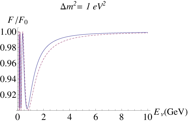
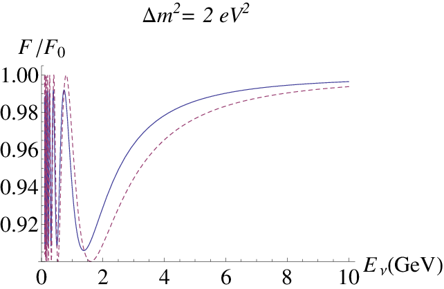
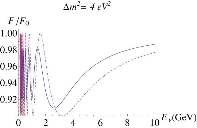
In Fig. 1 we show the effective probability $P_{eff}$, Eq. (18), as a function of neutrino energy for different values of $\Delta m^{2}_{42}$. For comparison we also show the standard probability with baseline $L$. A few comments are in order.

1. 1.

   Due to the large size of the neutrino production region, (and the effect of partial decoherence at the production) positions of the first and higher oscillation minima are shifted to lower energies in comparison with pointlike production case with baseline $L$. The relative shift increases with $\Delta m^{2}_{42}$ and decreases with energy.

2. 2.

   The depth of oscillations is suppressed due to the decoherence effect in comparison to the standard oscillation case. This suppression becomes stronger with increase of $\Delta m^{2}_{42}$ and therefore $\xi$, and decrease of energy.

3. 3.

   For characteristic neutrino energy $E_{\nu}=2$ GeV (responsible for the observed events with energy $\sim 1$ GeV) and $\Delta m^{2}_{42}=1$ eV² the oscillation effect in the ND is $P_{ND}\simeq 0.97$, as compared to the average suppression, $P_{FD}=0.95$, in the FD. Therefore $P_{FD}/P_{ND}=0.98$ instead of $0.95$ without oscillations in ND. So, clearly for this $\Delta m^{2}_{42}$ the bound on mixing parameter should be substantially weaker. For $\Delta m^{2}_{42}=0.5$ eV² the oscillation effect is 0.008 and the corresponding ratio, $P_{FD}/P_{ND}=0.96$, is close to the result which MINOS uses.

In this section, we find the oscillation effect assuming that neutrinos are coherently emitted along the pion trajectory. We will integrate the amplitude of oscillation over the production region and then compute the probability of the process.

But before that, let us elaborate more on the decoherence parameter $\xi$. According to the exact energy-momentum conservation in the decay process the difference of energies of the neutrino mass eigenstates equals in the pion rest frame

$$\Delta E_{42}^{0}=\frac{\Delta m_{42}^{2}}{2m_{\pi}}.$$

(23)

This difference is comparable with the width

$$\Delta E_{42}^{0}\sim\Gamma_{0}$$

(24)

at $\Delta m_{42}^{2}\sim 7$ eV². The ratio of the two parameters,

$$\frac{\Delta E_{42}^{0}}{\Gamma_{0}}=\frac{\Delta m_{42}^{2}}{2m_{\pi}\Gamma_{0}}=\alpha\xi,$$

(25)

coincides with the coherence parameter up to factor $\alpha\sim 0.45$. Notice that the difference of momenta of the eigenstates is even bigger:

$$\Delta p_{42}^{0}=-\frac{\Delta m_{42}^{2}}{2m_{\pi}}\cdot\frac{m_{\pi}^{2}+m_{\mu}^{2}}{m_{\pi}^{2}-m_{\mu}^{2}}~.$$

(26)

Numerically,

$$\xi\approx 0.33\left(\frac{\Delta m_{42}^{2}}{1{\rm eV}^{2}}\right).$$

(27)

For $\xi\gg 1$ the energy splitting is larger than the uncertainty in energy, and therefore the neutrino mass eigenstates are produced incoherently.

This consideration practically does not depend on the reference frame since violation of coherence is a physical phenomenon. In a frame where the pion moves with the Lorentz factor $\gamma_{\pi}$ and neutrinos are emitted in the direction of pion we have $\Gamma_{0}\rightarrow 2\gamma_{\pi}\Gamma_{0}$, and

$$\Delta E_{42}^{0}\rightarrow 2\gamma_{\pi}\Delta E_{42}^{0}\,\frac{m_{\pi}^{2}}{m_{\pi}^{2}-m_{\mu}^{2}},$$

(28)

so that the ratio changes roughly by a factor of 2 [6].

If $\xi\ll 1$ the mass eigenstates are produced in the coherent state. In the MINOS case we deal with the intermediate situation when results depend on the shape of the wave packet of neutrino. Indeed, the expression in Eq. (13) depends on the exponential decay factor, which turns out to be the shape factor of the neutrino wave packet (squared) from free pion decay.

In a reference frame where the pion has energy $E_{\pi}$ the decay length equals $l_{dec}=E_{\pi}/(m_{\pi}\Gamma_{0})=E_{\nu}/(\alpha m_{\pi}\Gamma_{0})$, and the oscillation length of neutrinos $l_{\nu}=4\pi E_{\nu}/\Delta m^{2}_{42}$. The ratio of the two lengths

$$\frac{l_{dec}}{l_{\nu}}=\frac{\Delta m^{2}}{4\pi\alpha m_{\pi}\Gamma_{0}}=\frac{\xi}{2\pi}$$

(29)

equals up to the factor $1/2\pi$ the decoherence parameter. Therefore the condition of coherence is $l_{dec}\ll l_{\nu}$.

Consistent treatment of decoherence effects can be done in terms of wave packets. The produced $\nu_{\mu}$ state can be described as

$$|\nu_{\mu}(x,t)\rangle=\sum_{i}U_{\mu i}^{*}\Psi_{i}(x,t)|\nu_{i}\rangle=\sum_{i}U_{\mu i}^{*}g_{i}^{S}(x-v_{i}t)e^{ip_{i}x-iE_{i}t}|\nu_{i}\rangle,$$

(30)

and for the detected state we have

$$|\nu_{\mu}(L-x)\rangle=\sum_{k}U_{\mu k}^{*}g_{k}^{D}(x-L)e^{ip_{k}^{\prime}(x-L)}|\nu_{k}\rangle.$$

(31)

Here, $\Psi_{i}(x,t)$ is the wave function of the mass eigenstate and $\nu_{i}$, $g_{i}^{S}$ and $g_{i}^{D}$ are the shape factors of the neutrino wave packets which correspond to the production and detection of the $i$th mass eigenstate. Also, $p_{i}$ and $p^{\prime}_{i}$ are the mean momenta of the these wave packets, $E_{i}=\sqrt{p_{i}^{2}+m_{i}^{2}}$ and $v_{i}$ is the group velocity of $i$th mass eigenstate (see [7] for details).

We now show that under certain assumptions the wave packet calculation leads to the same result as in Sec. 2. In the case of neutrinos produced in pion decay the neutrino wave function in the space-time point $(x,t)$, as well as the shape factor $g_{i}^{S}$, can be found in the following way. The neutrino wave packet is formed as a result of an integration over the production region of partial plane waves emitted from each point of the region:

$$\Psi_{i}(x,\,t)=\int dx_{S}\int dt_{S}e^{-\frac{1}{2}\Gamma t_{S}}e^{ip_{i}(x-x_{S})-iE_{i}(t-t_{S})}.$$

(32)

Here $e^{-\frac{1}{2}\Gamma t_{S}}$ gives the amplitude of probability to find the pion at the moment of time $t_{S}$. Due to strong interactions the pion is produced in a small spacetime region around $x=0$, $t=0$ with very short wave packets. The production region is thus approximately described by a delta function

$$\delta(x_{S}-v_{\pi}t_{S}).$$

(33)

Furthermore, because the baseline is small for the ND, the spread of the wave packets due to the difference in group velocities is negligible. Therefore, the shape of the neutrino wave packet (exponential in this case) is conserved. The conservation of the shape implies in turn that there is a one-to-one correspondence between the points of the wave packet in a given point $(x,t)$ and in point $(x_{S},t_{S})$ at the production. This correspondence is expressed as

$$t\simeq\frac{x_{S}}{v_{\pi}}+\frac{x-x_{S}}{v_{\nu}}.$$

(34)

Here we take into account that before neutrino appears in the point $x,t$ pion travels distance $x_{S}$ from the origin with velocity $v_{\pi}$, and then neutrino travels distance $x-x_{S}$ with average group velocity $v_{\nu}$.

From Eqs. (34) and (33) we obtain

$$x_{S}(x,t)=\frac{v_{\pi}(v_{\nu}t-x)}{v_{\nu}-v_{\pi}},~~~~t_{S}(x,t)=\frac{x_{S}}{v_{\pi}}=\frac{(v_{\nu}t-x)}{v_{\nu}-v_{\pi}},$$

(35)

and the second equality leads to another delta function for $t_{S}$:

$$\delta\left(t_{S}-\frac{v_{\nu}t-x}{v_{\nu}-v_{\pi}}\right).$$

(36)

The two deltas, Eqs. (33) and (36), remove the integration over $x_{S}$ and $t_{S}$ in (32) giving

$$\Psi_{i}=e^{-\frac{1}{2}\Gamma t_{S}}e^{ip_{i}(x-x_{S})-iE_{i}(t-t_{S})},$$

(37)

where $x_{S}$ and $t_{S}$ are now functions of $x$ and $t$ as in Eq. (35). Therefore, according to Eq. (30), the shape factor equals

$$g_{i}^{S}(x-v_{\nu}t)=e^{-\frac{1}{2}\Gamma t_{S}}e^{-ip_{i}x_{S}+iE_{i}t_{S}},~~~t_{S}=t_{S}(x,t)\propto(v_{\nu}t-x).$$

(38)

The amplitude of probability of the $\nu_{\mu}$ detection is given by

	$\displaystyle A_{\mu\mu}(t)$	$\displaystyle=$	$\displaystyle\int dx\langle\nu_{\mu}(L-x)|\nu_{\mu}(x,t)\rangle$		(39)
		$\displaystyle=$	$\displaystyle\sum_{i}|U_{\mu i}|^{2}\int dxg_{i}^{S}(x-v_{i}t)g_{i}^{D*}(x-L)e^{ip_{i}L-iE_{i}t}e^{i(p_{i}-p_{i}^{\prime})(x-L)}.$		(40)

Since the size of the ND is much smaller than the decay pipe (production region) we can take $g_{i}^{D}(x-L)\propto\delta(x-L)$ and therefore

$$A_{\mu\mu}(t)=\sum_{i}|U_{\mu i}|^{2}g_{i}^{S}(L-v_{i}t)e^{ip_{i}L-iE_{i}t}.$$

(41)

The probability equals

$$P=\int_{-\infty}^{+\infty}dt|A_{\mu\mu}|^{2}=\int_{-\infty}^{+\infty}dt\sum_{i,k}g^{S}_{i}(L-v_{i}t)g^{S*}_{k}(L-v_{k}t)|U_{\mu i}|^{2}|U_{\mu k}|^{2}e^{i\phi_{ik}^{0}(L,t)},$$

(42)

where $\phi_{ik}^{0}(L,t)\equiv(p_{i}-p_{k})L-(E_{i}-E_{k})t\equiv\Delta pL-\Delta Et$ . Using the expressions for the shape factors in Eq. (38) we obtain

$$P=\int_{-\infty}^{+\infty}dte^{-\Gamma t_{S}(L,t)}\sum_{i,k}|U_{\mu i}|^{2}|U_{\mu k}|^{2}e^{i\phi_{ik}(L,t)},$$

(43)

where

$$\phi_{ik}(L,t)=\Delta p\big[L-v_{\pi}t_{S}(L,t)\big]-\Delta E\big[t-t_{S}(L,t)\big]$$

(44)

is the total phase difference between the mass eigenstates arriving at the detector in the moment of time $t$. The time factor in the last term of Eq. (44) can be rewritten as

$$t-t_{S}(L,t)=\frac{L-v_{\pi}t_{S}}{v_{\nu}}.$$

Then using the relation

$$\Delta E\approx v_{\nu}\Delta p+\frac{1}{2E}\Delta m^{2}$$

(45)

(which follows from the dispersion relation) we obtain

$$\phi_{ik}(L,t)=\frac{\Delta m^{2}}{2E}(L-v_{\pi}t_{S})$$

(46)

which exactly coincides with the standard oscillation phase. Inserting this expression into Eq. (43) and changing the integration variable $t$ to $x\equiv x_{S}=v_{\pi}t_{S}$, which varies in the limits $0-l_{p}$, we find

$$P\propto\int_{0}^{l_{p}}dxe^{-\Gamma x}P_{\mu\mu}(L-x).$$

(47)

This coincides (after normalization) with the expression found in Eq. (13). Thus, the result for completely coherent neutrino emission along the whole neutrino trajectory coincides with the case of completely incoherent emission which corresponds to very short wave packet of neutrino. Essentially, here we have a situation that resembles a coordinate-space version of the Kiers-Nussinov-Weiss theorem [8] where a fully incoherent ensemble of neutrino states is physically indistinguishable from neutrinos produced coherently if both cases lead to the same energy distribution.

If pions collide, the shape factor of the neutrino wave packet is not determined by the decay function of pion [9]. The coherent emission will occur only between two consecutive collisions with substantial momentum transfer. This usually leads to the Gaussian shape factor for the neutrino wave packet with the width $\sigma_{x}$ determined by mean free path of the pion. The consideration is simple if $\sigma_{x}$ is much smaller than the decay length: $\sigma_{x}\ll l_{decay}$. Suppose the pion emits a neutrino coherently in some region of size $\sigma_{x}$ centered at $x_{S}$. Then, instead of leading to Eq. (14), the integration over the emission region gives for the oscillation probability

$$P_{\mu\mu}(E_{\nu},L-x)=\bar{P}+S_{loc}(\sigma_{x}/l_{\nu})\frac{1}{2}\sin^{2}2\theta_{24}\cos[\xi\Gamma(L-x_{S})],$$

(48)

where $S_{loc}(\sigma_{x}/l_{\nu})$ is the localization factor. With collisions, it is this probability that should be used in computations of the neutrino flux in Eq. (13) and the integration should be performed over $x_{S}$. If $\sigma_{x}$ does not depend on $x_{S}$, in the final expression Eq. (18) $S_{loc}(\sigma_{x}/l_{\nu})$ appears as an additional factor at the oscillatory term. For $\sigma_{x}\ll l_{\nu}$ one has $S_{loc}\approx 1$ and Eq. (48) reproduces the original result. Another way to take into account the localization of pions is to perfom the averaging of the oscillatory term in Eq. (18) over the interval $\sigma_{x}$.

In the case $\sigma_{x}\sim l_{decay}$ one expects some interplay between exponential decay and decoherence due to finite $\sigma_{x}$ [9]. In this case in the limit $\sigma_{x}\gg l_{decay}$ one should obtain again our original result.

The number of the NC events with a given total energy of hadrons, $E_{h}$, equals

$$N(E_{h})=\int dE_{\nu}dxF_{\nu}(E_{\nu})\frac{d\sigma(E_{\nu},E_{h})}{dxdy},$$

(49)

where $\sigma(E_{\nu},E_{h})$ is the cross-section of production of hadrons with energy $E_{h}$ by neutrinos of energy $E_{\nu}$, $y\equiv E_{h}/E_{\nu}$ is the inelasticity and $x$ is the Bjorken variable. In what follows we will identify $E_{h}$ with the reconstructed energy $E_{reco}$ of [1]. We assume that $\sigma(E_{\nu},E_{h})$ is well approximated by the deep inelastic scattering cross-section of neutrinos off nucleons. We use the MSTW 2008 set for the parton distribution functions and the reported spectrum for the NuMI beam (see [10] for instance).

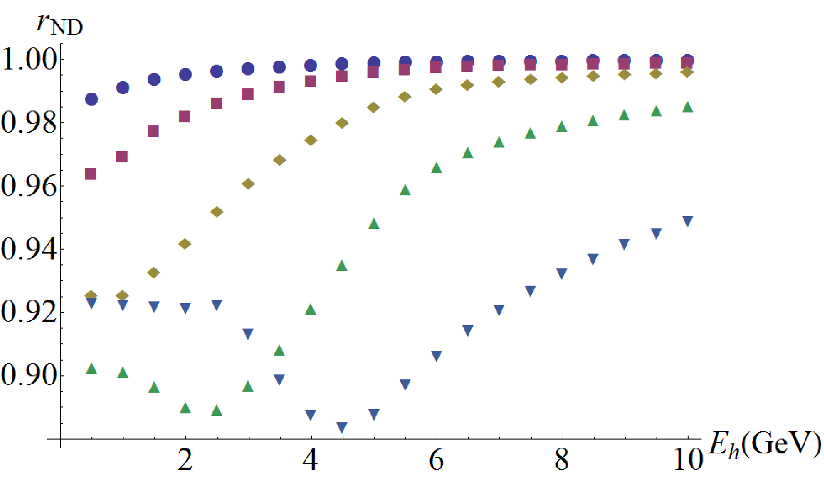
Let $N^{0}(E_{h})$ be the theoretical number of events computed according to Eq. (49) for $F_{\nu}=F_{\nu}^{0}$, i.e., as if there were no oscillations. We now define the ratio of events in the ND, with and without oscillations:

$$r_{ND}\equiv\frac{N(E_{h})}{N^{0}(E_{h})}\,.$$

(50)

The ratio $r_{ND}$ as a function of the hadron (“reconstructed”) energy is shown in Fig. 2. Its behaviour with varying $\Delta m_{42}^{2}$ can be separated in three regions:

1. 1.

   For $\Delta m_{42}^{2}<2\textrm{ eV}^{2}$ the peak of the spectrum of the incident neutrinos, $E_{\nu}\sim 3.3$ GeV, is in the region of small oscillation effect, (see Fig. 1), and $r_{ND}\sim 1$ for most of the $E_{h}$ range. The oscillation minimum is below $E_{\nu}\sim 2$ GeV and, therefore, there is some depletion of events with energy $E_{h}<2$ GeV. Nevertheless, $r_{ND}$ remains bigger than $\bar{P}$ for the whole energy range.

2. 2.

   For $2\textrm{ eV}^{2}<\Delta m_{42}^{2}<8\textrm{ eV}^{2}$ the dip in the oscillation probability falls in the region of energies for which the neutrino beam has maximum intensity. There is a considerable depletion of events for neutrino energies below $5$ GeV and $r_{ND}<\bar{P}$ in this region. We will see below that, in this case, an excess of events should be observed in the FD compared to MINOS simulations.

3. 3.

   For $\Delta m^{2}_{42}>8\textrm{ eV}^{2}$ the first oscillation minimum is above the peak of the neutrino spectrum and the averaging is substantial for low $E_{h}$. Still, for $\Delta m^{2}_{42}<15\textrm{ eV}^{2}$ there are noticeable deviation from $\bar{P}$ below $E_{h}=5$ GeV as MINOS becomes sensitive to higher oscillation minima.

The Monte Carlo prediction $N_{ND}^{0}$ for the number of events in the ND without oscillations, (see Fig. 1 in [1]), needs to be corrected when the oscillations into sterile neutrino are present as

$$N_{ND}=r_{ND}~N_{ND}^{0}\,.$$

(51)

At

$$\Delta m_{42}^{2}=(1-3)~{\rm eV}^{2},~~~\sin^{2}2\theta_{24}=0.15-0.20\,,$$

(52)

the oscillations can explain the deficit of events in the ND in the low energy bins (see Fig. 3). This deficit is not yet statistically significant and for ND it is below the systematic errors. However the oscillations at ND must be taken into account when oscillation effect “propagates” from ND to FD.

In Fig. 3 we show distributions of events over the reconstructed hadron energy $E_{h}$ in the ND for different values of $\Delta m^{2}_{42}$ (Eq. (53)). Also shown is the distribution without oscillations $N_{ND}^{0}$ from [1] and experimental points.

The MINOS collaboration predicts the number of events in the FD, $N_{FD}^{0}$, extrapolating the experimentally measured spectrum at the ND. In [1] it is assumed that oscillation effects are absent in the ND but the effect of the usual $3\nu$ oscillations at the FD is included (see Fig. 2 in [1]). The averaged $\nu_{\mu}-\nu_{s}$ oscillations in the FD modify this prediction: $N_{FD}^{0}\rightarrow\bar{P}N^{0}_{FD}$. However, when oscillations at the ND are taken into account, the latter must be corrected consistently with Eq. (51):

$$N_{FD}=\frac{\bar{P}}{r_{ND}}~N_{FD}^{0}\,.$$

(53)

Thus, the factor

$$R(E_{h})=\frac{\bar{P}}{r_{ND}}.$$

(54)

is the conversion factor for the flux predicted at the FD with and without of $\nu_{\mu}-\nu_{s}$ oscillations.

The behavior of $R(E_{h})$ can be straightforwardly inferred from Fig. 2. Again, there are three different cases:

1. 1.

   Averaged effect in ND: $R(E_{h})\approx 1$. This happens at low energies for large $\Delta m_{42}^{2}$ when one has the averaged oscillation effect in the ND. The MINOS prediction for the number of events at the FD is unchanged by $\nu_{\mu}-\nu_{s}$ oscillations.

2. 2.

   Strong suppression in ND: $R(E_{h})>1$. The neutrino energies in the peak of the neutrino flux are around the first oscillation minimum for $2\textrm{ eV}^{2}<\Delta m_{42}^{2}<8\textrm{ eV}^{2}$. In this case one predicts some excess of events in the FD in comparison to the MINOS extrapolation which can partially explain the observed excess (see Fig. 3)

3. 3.

   Weak effect in the ND: $R(E_{h})<1$. This regime is realized for neutrino energies above the first oscillation minimum for all mass squared differences. It corresponds to small or no oscillation effect at the ND.

In Fig 3 we show the distribution of events in the reconstructed hadron energy, $E_{h}$ in the FD for different values of $\Delta m^{2}_{42}$ (Eq. (55)) Also shown is the distribution without oscillations $N_{ND}^{0}$ from [1] and experimental points.

We consider next how the bounds on the $\nu_{\mu}-\nu_{s}$ mixing are modified for different $\Delta m_{42}^{2}$. For $\Delta m_{42}^{2}<0.5$ eV² the decoherence is negligible, the oscillation effects in ND are significant only at low energies and therefore the MINOS limit in Eq. (1) is approximately valid. For $\Delta m_{42}^{2}>0.5$ eV² the limit should be modified. The strongest modification is for $\Delta m_{42}^{2}=(2-8)$ eV², when the first oscillation minimum is at neutrino energies $E_{\nu}$ that correspond to the peak in the spectrum of events. Notice that Eq. (52) corresponds to $\theta_{24}\sim(11-13)^{\circ}$ which is substantially larger than the limit in Eq. (1).

We stress that the calculations performed in this section are meant for illustration purposes. For precise quantitative results one should perform a complete MC simulation of events without the simplifications we made.

In this work we considered the oscillation effects in the ND of the MINOS experiment. The MINOS setup realizes an interesting situation of partial decoherence of the neutrino state at the production, when the energy splitting of two mass eigenstates is comparable with the energy uncertainty of the initial state (the width of pion). Decoherence leads to suppression of the oscillation effect at high energies (above the oscillation minimum), to the shift of oscillation minimum (dip) to low energies and to suppression of the depth of oscillations. The suppression becomes stronger at low energies. In general, the effect of decoherence should be taken into account for all experiments that perform searches for sterile neutrinos with 1 eV mass using neutrino beams from pion decays.

The MINOS bounds, Eq. (1) remain valid for $\Delta m^{2}_{42}<0.5$ eV². For $\Delta m^{2}_{42}>0.5$ eV² the oscillation effect in the ND should be taken into account. It should noticeably weaken the bounds for $\Delta m^{2}_{42}>2$ eV². An estimation of this effect has been performed in this paper; a full quantitative analysis should be done by the MINOS collaboration. For $\Delta m^{2}_{42}>15$ eV² the bound disappears and MINOS is insensitive to the $\nu_{\mu}-\nu_{s}$ oscillations.

The MINOS data might actually provide a hint of oscillations with $\Delta m^{2}_{42}\sim(1-3)$ eV². The oscillations can explain some deficit of signal in the low energy bins of the ND as compared to the Monte Carlo prediction, and the excess of events in the FD.

The authors are grateful to E. Kh. Akhmedov for very useful discussions.

Using the Lorentz transformation to the laboratory frame we have for neutrino momenta:

$$p_{y}=p_{0}\sin\theta_{0},~~~p_{x}\approx p_{0}\gamma_{\pi}(\cos\theta_{0}+\beta_{\pi}),$$

(55)

where $\theta_{0}$ is the neutrino angle of emission in the pion rest frame; $\gamma_{\pi}\equiv E_{\pi}/m_{\pi}$ is the Lorentz factor of the pion and $\beta_{\pi}$ is the pion velocity. The neutrino energy in the laboratory frame, $E_{\nu}=\sqrt{p_{x}^{2}+p_{y}^{2}}$, in the aproximation of $\gamma_{\pi}\gg 1$ can then be written as

$$E_{\nu}\approx E_{0}\gamma_{\pi}(\cos\theta_{0}+\beta_{\pi})\approx E_{0}\gamma_{\pi}(\cos\theta_{0}+1).$$

(56)

Therefore,

$$\alpha\approx\frac{E_{0}}{m_{\pi}}(\langle\cos\theta_{0}\rangle+1).$$

(57)

To evaluate the effective value of the angle $\langle\cos\theta_{0}\rangle$ let us consider the real experimental setup. According to Eq. (55), the angle between the neutrino and pion in the laboratory frame equals

$$\tan\theta_{\nu}=\frac{\sin\theta_{0}}{\gamma_{\pi}(\cos\theta_{0}+1)}.$$

(58)

Consequently

$$\cos\theta_{0}=\frac{1-b}{1+b},~~~b\equiv\gamma_{\pi}^{2}\tan^{2}\theta_{\nu}.$$

(59)

The maximal value of $\tan\theta_{\nu}$ is given by

$$\tan\theta^{max}=\frac{r}{L-x}$$

(60)

with $r\approx 1$ m being the radius of the fiducial zone of the ND and $L$ is the distance from the target to the ND. It equals $2.5\times 10^{-3}$ for $x=l_{p}$ and and $10^{-3}$ for $x=L$. So, for the typical pion energy $E_{\pi}=10$ GeV we find the effective distance $\bar{x}=300$ m and $b=0.01$, and therefore $\cos\theta_{0}\sim 0.98$. We have checked that results do not change substantially for different values of $\alpha$.

References

- [1] P. Adamson et al. [ MINOS Collaboration ], [arXiv:1104.3922 [hep-ex]].
- [2] A. Aguilar et al. [ LSND Collaboration ], Phys. Rev. D64 (2001) 112007. [hep-ex/0104049].
- [3] A. A. Aguilar-Arevalo et al. [ The MiniBooNE Collaboration ], Phys. Rev. Lett. 105 (2010) 181801, [arXiv:1007.1150 [hep-ex]].
- [4] D. Meloni, J. Tang, W. Winter, Phys. Rev. D82 (2010) 093008. [arXiv:1007.2419 [hep-ph]].
- [5] P. Adamson et al. [The MINOS Collaboration], Phys. Rev. D 81 (2010) 052004 [arXiv:1001.0336 [hep-ex]].
- [6] Y. Farzan and A. Y. Smirnov, Nucl. Phys. B 805 (2008) 356 [arXiv:0803.0495 [hep-ph]].
- [7] E. K. Akhmedov and A. Y. Smirnov, Phys. Atom. Nucl. 72 (2009) 1363 [arXiv:0905.1903 [hep-ph]].
- [8] K. Kiers, S. Nussinov and N. Weiss, Phys. Rev. D 53 (1996) 537 [arXiv:hep-ph/9506271].
- [9] E. K. Akhmedov D. Hernandez and A. Yu. Smirnov, in preparation.
- [10] S. E. Kopp, AIP Conf. Proc. 967 (2007) 49-52.