Slow Dynamics of the High Density Gaussian Core Model
Abstract
We numerically study crystal nucleation and glassy slow dynamics of the one-component Gaussian core model (GCM) at high densities. The nucleation rate at a fixed supersaturation is found to decrease as the density increases. At very high densities, the nucleation is not observed at all in the time window accessed by long molecular dynamics (MD) simulation. Concomitantly, the system exhibits typical slow dynamics of the supercooled fluids near the glass transition point. We compare the simulation results of the supercooled GCM with the predictions of mode-coupling theory (MCT) and find that the agreement between them is better than any other model glassformers studied numerically in the past. Furthermore, we find that a violation of the Stokes-Einstein relation is weaker and the non-Gaussian parameter is smaller than canonical glassformers. Analysis of the probability distribution of the particle displacement clearly reveals that the hopping effect is strongly suppressed in the high density GCM. We conclude from these observations that the GCM is more amenable to the mean-field picture of the glass transition than other models. This is attributed to the long-ranged nature of the interaction potential of the GCM in the high density regime. Finally, the intermediate scattering function at small wavevectors is found to decay much faster than its self part, indicating that dynamics of the large-scale density fluctuations decouples with the shorter-ranged caging motion.
I Introduction
Essential aspects of the glass transition of the supercooled liquids remain still elusive despite of decades of study. Many theories and scenarios have been proposed to explain the dramatic slow down of the systems and the associated growing cooperative length scales near the glass transition point [1, 2, 3, 4]. They can explain the experimental results equally well or equally poorly but none of them have been proved to be decisively better than other. Even a satisfactory mean-field picture of the glass transition has not been established [5, 6]. Numerical simulation of simple model fluids is an ideal route to examine the competing theories. Considerable efforts have been put forward to gain insight from the dynamical behaviors of simple model glassformers in silico, but compelling answers are still lacking. There are several reasons why the simulation studies are not successful in sorting out numerous scenarios and theories. First, the model systems are more or less similar; the pair potentials of canonical glassformers studied in the past are exclusively characterized by short-ranged strong repulsions. Examples are Lennard-Jones, its WCA counterpart, soft-core, and the hard sphere potentials. Since the strong repulsion dominates thermodynamic and dynamic properties of dense fluids, it is hardly surprising that the results for these models are qualitatively similar [7, 8]. Studies of a completely different class of potential systems may potentially diversify our views and perspectives on the glass transition within the limited accessible time windows of the simulations. Secondly, the model systems are not clean enough. Even the simplest class of model glassformers (with a few exceptions [9, 10]) are inevitably bidisperse or polydisperse in order to avert the nucleation to the crystalline phase [7]. This complicates quantitative assessment of the simulation results. Finally, we still lack a realistic model glassformer which conforms to the mean-field picture in finite dimensions. Concept of the mean-field scenario of the structural glass transition is basically borrowed from the mean-field theory developed in the spin glass communities [11, Cavagna2009, 3, 4]. The replica theory [12, 13] and mode-coupling theory (MCT) [14] are believed to be the static and dynamic versions of the mean-field theory of the glass transition, simply because of their apparent resemblance to the spin-glass counterparts. The mosaic pictures of the random first order transition theory has been developed as the finite dimension version of this mean field pictures [11, 15, 3]. Accumulated simulation data are not inconsistent qualitatively from the prediction of the mean field theories but the quantitative agreement between simulation results and theoretical predictions are far from compelling. The best way to verify the mean-field scenario would be to take the mean-field limit by either going to higher dimensions or making the system’s interactions longer-ranged. Recently, simulations for four dimensional systems have been performed [16, 10]. Results therein hint that the dynamic heterogeneities are suppressed compared with three dimensional systems and agreement with MCT moderately improves [10]. However, considering the current computational abilities, it would be hard to simulate the system beyond four dimension, whereas the upper critical dimension of the glass transition is argued to be eight [17, 18]. On the other hand, few studies have been done for realistic liquids with long-ranged particle interactions [19, 20, 21].
The Gaussian core model (GCM) is a candidate to dispel all of the above-mentioned concerns and could be an ideal and clean bench to compare with various glass theories. The GCM consists of the point particles interacting with a Gaussian shaped repulsive potential [22, 23, 24, 25, 26, 27, 28, 29, 30, 31];
| (1) |
where is the interparticle separation, and are the parameters which characterize the energy and length scales, respectively. The GCM is one of the simplest models of the so-called ultrasoft potential systems which are characterized by the bounded and long-tailed repulsive potential [32]. Recently, we have reported that the one-component GCM vitrifies at very high densities [33]. The GCM or the ultrasoft particles in general have very distinct and exotic properties both thermodynamically and dynamically [22, 23, 24, 25, 26, 27, 28, 29, 30, 31, 33, 34], such as the re-entrant melting at high densities, negative thermal expansion coefficient, and anomalous density dependence of the diffusion coefficient. There are several studies on the glass transition of the ultrasoft particles [35, 36, 37, 38] and it was found that they exhibit rich dynamical behaviors different from conventional model glassformers [35, 36]. One of the advantages to study the glass transition of the ultrasoft particles is that, due to the mild repulsion tail of the potential, the density as well as the temperature can be used as a parameter to control the system. Exploring the wide range of density–temperature parameter space makes it easier to establish various scaling laws, to bridge the gaps between temperature-driven ordinary glasses and density-driven colloidal glasses, and to help unifying the concepts of the finite-temperature glass transition and the zero-temperature jamming transition [37, 38]. However, most studies in the past focused on the relatively low density regime, where the generic nature of the glass transition is not extremely different from that of the conventional model glassformers. The systems at low densities, including the GCM, also had to be either polydisperse or bidisperse in order to avoid crystallization.
The GCM at very high densities is very different [33]. First of all, the system vitrifies without poly(bi)dispersity. The nucleation rate systematically decreases as the density increases and the system starts exhibiting typical slow dynamics observed in supercooled fluids near the glass transition point. Furthermore, the dynamics is quantitatively well-described by MCT. Especially, the MCT nonergodic transition point extracted from the simulation unprecedentedly matches with the theoretical prediction. Besides, the violation of the Stokes-Einstein relation and the amplitude of the non-Gaussian parameter, both of which is the manifestation of the heterogeneous fluctuations of dynamics, are suppressed. We conjecture that these facts can be attributed to the long-ranged nature of the interaction potential at the high densities where particles are overlapped. These results suggest that the high density GCM is not only one of the cleanest model glassformers in silico, but also the closest to the mean-field model.
In this paper, we present thorough and complete numerical analysis of the nucleation and glassy dynamics of the high-density and one-component GCM. We not only present the exhaustive set of the numerical results but also provide with the new evidence which bolsters the validity of MCT. Detailed analysis of thermodynamic and structural properties of the high density GCM, such as the phase diagram and the static structure factors are discussed in Ref. [34]. In the previous study [33], we have attributed the weak violation of the SE relation and smaller non-Gaussian parameter to the suppression of the dynamic heterogeneities. We provide stronger and more direct evidence that intermittent heterogeneous motion is suppressed by monitoring the distribution of the particle displacement as a function of time. We also evaluate the correlation functions of single and collective density fluctuations. Surprisingly we find that dynamics of the collective density decouple from the single particle density at large length scales, where the former relaxes much faster than the latter. This is in stark contrast with the ordinary model glassformers for which the slow glassy dynamics set in over the whole length scales for both collective and single particle densities alike. We compare these simulation results with MCT predictions and find that MCT beautifully captures the decoupling of dynamics at the large length scales. However, we also find a subtle but noticeable disagreement of MCT from the simulation results at intermediate length scales, where the nonergodic parameter (the plateau height of the two step relaxation in the density correlators) predicted by MCT shows a weak shoulder which tends to grow as the density increases. This shoulder is reminiscent of those found for the -dimensional hard sphere glasses at large evaluated from MCT [5, 6] and may be a signal of breakdown of MCT at the mean field limit.
This paper is organized as follows. In Sec. II, we summarize the simulation method, theoretical background, and the setting of the system. The nucleation dynamics from fluid to crystalline phase is discussed in Sec. III. In Sec. IV, we present all simulation results on various static and dynamical observables. Detailed analysis and careful comparison of the simulation results with the MCT predictions are made. Suppression of the dynamic heterogeneities are also discussed. Finally, Sec. IV concludes the paper with a summary.
II Preliminaries
II.1 Simulation Methods

We investigate the dynamics of the one-component GCM using a molecular dynamics (MD) simulation in the ensemble with a Nosé thermostat. The system is a cubic cell and a periodic boundary condition is imposed. A time-reversible integrator, similar to the velocity-Verlet method, is used with a potential cut-off at [39]. Hereafter, , , and are taken as the units of the length, temperature, and time, respectively. The time step is fixed at 0.2, which is sufficiently small to conserve the Nosé Hamiltonian during the long simulation runs. We focus on the four densities, , , , and , and perform the MD simulations for various temperatures in the vicinity of the melting temperature . The state points which we performed simulation are shown in Fig. 1 along with the solid-fluid phase boundary line [26, 33, 34]. As discussed in detail in the previous study [34], the melting temperature, , at the high density regime obeys an asymptotic scaling which was originally conjectured by Stillinger [22]. For all densities which we study, thermodynamically stable crystalline structure is bcc [33, 34]. We run the simulations for the total run time always 50 times longer than the structural relaxation time. For example, the simulation time was for the lowest temperature at . This was confirmed to be sufficiently long to neglect aging effect. The first half of the simulation run was used for the equilibration and we used the trajectories of the second half for the analysis of the stationary dynamics. For each state point, five independent runs are performed and the results are obtained by averaging over those trajectories in order to improve the statistics. Configurations obtained from the high temperature simulation were used as the initial configurations. The system size is fixed at . The simulations for and confirmed that the finite-size effect is negligible.
II.2 Mode Coupling Theory
In this work, we compare our simulation results for dynamics of the high density GCM in the supercooled state with the prediction of MCT. In the context of the glass transition, MCT is commonly expressed as a set of the self-consistent nonlinear equations for correlation functions. These correlation functions are the intermediate scattering function (the correlation of the collective density), , where is the -dependent density fluctuation, and the self intermediate scattering function or the correlation of the single particle density, , where is the density of a single particle. The time evolution of is given by the generalized Langevin equation
| (2) |
where is the frequency term. is the static structure factor. is the memory kernel which, according to MCT, is approximated as
| (3) |
Here is the vertex, where is the direct correlation function. In Eq. (3), we neglect the short time contribution for the memory kernel, which does not affect the slow dynamics. MCT predicts that undergoes the ergodic-nonergodic transition at a finite temperature, , below which remains finite. is referred to as the nonergodic parameter. The nonergodic parameter and can be evaluated by taking of Eqs. (2) and (3), which is expressed as
| (4) |
where is the long time limit of the memory kernel. As the temperature approaches to from above, MCT first predicts that exhibits the two-step relaxation behavior characterized by a finite plateau and the slow structural relaxation. The height of the plateau is identical to at . The structural relaxation or the alpha relaxation time, , increases and eventually diverges at . MCT predicts that the increase of is given by a power law , where is a system-dependent parameter which can be evaluated from the MCT equation.
Likewise, the MCT equation for the self intermediate scattering function, , is written in the same form as Eq. (2), but with the frequency term instead of and the self memory kernel
| (5) |
instead of in Eq. (3). The MCT equation for undergoes the nonergodic transition exactly at the same temperature, , as for , at least for most model systems studied in the past (see Ref. [40] for exceptions). By taking the small -limit of the MCT equation for , we can also construct the self-consistent equation for the mean square displacement . MCT predicts that the self-diffusion coefficient follows the power law and vanishes at . Note that the power law exponent is identical with that for . In addition to the MCT nonergodic transition and power law of the transport coefficients, MCT predicts many important dynamical properties such as the dynamic scaling known as von Schweidler’s law at the plateau regime (the beta regime) and the time-temperature superposition at the alpha relaxation regime [41].
III Crystallization
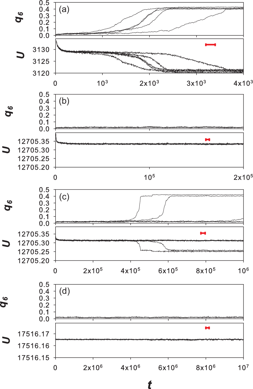
Ordinary simple atomic fluids nucleate to form crystals quickly as the temperature is lowered below the melting point. In this section, we analyze the crystal nucleation dynamics of the high density GCM and show that the nucleation rate systematically decreases as the density increases. In order to monitor the crystallization from the homogeneous fluid phase, we use the potential energy and the bond order parameter [42]. The bond order parameter is defined by
| (6) |
where is the -th bond order parameter of the -the particle defined by
| (7) |
Here is the complex bond parameter of the -th particle given by
| (8) |
where is the position of the -th particle, is the number of nearest neighbor particles around the -th particle, and is the spherical harmonic function of the degree and the order .
is zero in the fluid phase and for a perfect bcc crystal [42]. In Fig. 2, we show and of the five representative trajectories as a function of the lapse of time measured from the moment when the system is prepared. At a relatively low density and temperature just below the melting point (Fig. 2 (a)), one observes that ’s of all five trajectories abruptly increase from zero to a finite value and concomitantly ’s decrease. These behaviors are the hallmark of the crystal nucleation. This figure shows that the nucleation initiates only after the lapse of time several times longer than the structural relaxation time which is indicated by the short bold lines in the figures (the precise definition and compiled data set of are given in Sec. IV). The degree of supersaturation defined by at this state point is 0.43. Next, we look at the higher density . Five runs of and at are shown in Fig. 2 (b). Despite of the deeper supersaturation () and much longer simulation runs (over 40 ) than Fig. 2 (a), and do not show any sign of nucleation. Decreasing the temperature further to where (Fig. 2 (c)), one eventually observes the crystallization for the two out of five trajectories. Note that it takes decades of the structural relaxation time (which itself also increases with the degree of supersaturation) before the precipitous nucleation takes place. At even higher density , all five trajectories fail to nucleate even at a very low temperature with the similar degree of the supersaturation, , for the whole simulation runs.

In order to ensure that the nucleated samples are unambiguously the bcc crystal and that samples which failed to nucleate remain in the homogeneous fluid phase, we evaluate new parameters which were recently introduced by Lechner et al. [43]. They have used the two averaged bond order parameters and and demonstrated that the correlation map of them improves ability to determine the crystalline structures [43, 44]. The averaged bond order parameter is defined by replacing in Eq. (7) with the averaged value defined by
| (9) |
where is given by Eq. (8) and the sum runs from over all neighbors of the -th particles, including the -th particle itself ( in the sum). In Fig. 3, we placed all and () in the correlation map for the configurations obtained at the end of simulation runs of the two state points and . The four circles represent the characteristic areas for the bcc, hcp, fcc crystals, and fluid phase [43]. The results for show that the two trajectories remain in the fluid phase whereas the rest formed the bcc crystal. It is clear that no other structures are formed in the course of the simulations. Note that the results for the three trajectories which nucleated slightly deviate from the bcc region, which we presume is due to defects or imperfectness of the obtained crystalline structures. On the other hand, all the five trajectories for do not show any hint of crystal nucleation and the configurations remain completely disordered. Hereafter, we focus on the densities and 2.0 because the crystal nucleation is sufficiently slow that canonical glassy dynamics are observed.
IV Glassy Dynamics
IV.1 Structural functions

Before discussing the slow dynamics in the supercooled state, we summarize the fluid structures of the high density GCM to demonstrate the difference from those of conventional model glassformers. In Fig. 4, we plot the radial distribution functions and static structure factors of the GCM for and 2.0 near and below the melting temperatures. Both and show typical behaviors of dense fluids characterized by the prominent peaks near the position and the wavevector corresponding to the first coordination shell. Their peak heights increase as the temperature decreases. As density increases from to 2.0, the peak position of shifts from to 0.85 and for from to 8.4. The noticeable feature of the high density GCM is that the tail of the potential stretches beyond the first coordination shell, as demonstrated in Figs. 4 (a) and (c). This considerable overlap of particles imparts the character of the long-ranged interaction systems to the high density GCM. The long-ranged nature also appears as the anomalously small at small wavevectors. The insets of Figs. 4 (b) and (d) show that , or the compressibility, is far smaller than the other model fluids at compatible supersaturations, implying that the density fluctuations at large length scales are strongly suppressed. This is the common features of the long-range interacting systems. A well-known example is the one component classical plasma [45], where vanishes at . More detailed analysis of the simulation results for the structural functions and comparisons with the predictions of the liquid state theory have been reported in Ref. [34]. ’s obtained here are used in the MCT analysis discussed below.
IV.2 Mean square displacement and self intermediate scattering function


In this subsection, we evaluate various dynamic quantities and observe their slow dynamics, focusing on the trajectories which did not crystallize even when deeply supercooled. The mean square displacement , the self intermediate correlation function , and the intermediate correlation function are evaluated for the densities and 2.0. Fig. 5 shows and at several temperatures well below the melting temperature. These figures clearly display the canonical behaviors of the supercooled liquids near the glass transition point. For , we could not observe the glassy dynamics below because the crystallization intervened. At , all trajectories did not crystallize down to the lowest temperature which we accessed. In Figs. 5 (a) and (c), one observes that, as the temperature is lowered, develops the long plateau regimes followed by the usual diffusive behaviors at longer times. The appearance of the plateau signals the formation of a cage of a particle surrounded by its neighbors and is the hallmark of the supercooled fluid near the glass transition point. The value of at the plateau region is a measure of the sizes of the cages. They are about 0.17 for and 0.14 for . These values are slightly smaller than the values for conventional model glassformers. For example, for the Kob-Anderson Lennard-Jones mixture (KA model) [46].
In Fig. 5 (c) and (d), we plot for several temperatures, where is the wavevector where show the maximum peak. relaxes exponentially at high temperatures. As the temperature decreases, a plateau with a finite height appears and it stretches over longer times as the temperature decreases further, while the plateau height remains almost constant. This two-step relaxation behavior is another hallmark of the slow dynamic near the glass transition point. The terminal relaxation following the plateau is called the structural or alpha relaxation. We define the structural relaxation time by . In Fig. 6, we plot against the time scaled by . The result shows that relaxation curves are collapsed at the alpha relaxation regime. This is the universal property of the glassy systems known as the time-temperature superposition (TTS) [41]. Furthermore, the all curves where TTS holds are fitted by a stretched exponential function with the exponent . This value is comparable with that for the KA model [46] and for the hard sphere mixture [47].

In Fig. 7, the structural relaxation time and the self diffusion constant defined by are plotted against the inverse temperature. We plotted and adjusted its ordinate so that the data collapses with at high temperatures. For both densities, and , and drastically increase as the temperature is lowered. Both data almost collapse to each other for the whole temperatures except for the slight deviation at the lowest temperature. As we shall discuss later, this is the direct reflection of a weak violation of the Stokes-Einstein relation.
So far, all simulation data show no sign of peculiarity in the slow dynamics of the high density GCM at the qualitative level. They are all similar to conventional model glassformers. In order to assess the properties of the high density GCM more quantitatively, we compare the simulation results with the predictions of MCT. For this purpose, we solve the MCT equations Eqs. (2)–(5) by numerically integrating the equations in a self-consistent manner. As inputs, we used obtained numerically in the previous subsection. First, we compute the MCT transition temperature by solving Eq. (4). The results are and for and 2.0, respectively. Here, we denote the transition temperature as in order to emphasize that they are obtained by solving the MCT equations. The exponent is also obtained from the MCT solutions.
MCT predicts that both the self-diffusion coefficient and the structural relaxation time follow the power law with the same parameters and . We fitted and obtained by simulation with this MCT power law, using as a fitting parameter. We denote it as . By plotting and against , we found that they both vanish at the same temperature and we identified and for and 2.0, respectively (see the insets of Fig. 7). In Fig. 8, we replotted in Fig. 7 using instead of . The results for the KA model [46] are also plotted. These data are scaled by a time unit, , defined by a relaxation time at the short time scale, . This figure shows that the relaxation times for both the GCM and KA model ride on the MCT power law for the range of temperatures which the simulation can access. Collapse of the data of two systems on a single power law is a reflection that the values of ’s of both systems are close ( for the KA model [48]). This figure also demonstrates that is a good parameter to measure the distance from the onset of the glassy slow dynamics for different systems. Hereafter, we refer to as the reduced temperature. In Fig. 5 (c), we plotted the simulation data of for the KA model at by shifting the time unit in such a way that the long time diffusive regime collapses with the data for the GCM at and whose reduced temperature is about the same. Almost perfect collapse of the results for two distinct systems for the whole time window, including the short time ballistic behavior and the entry to the plateau regime, suggests that the slow diffusive behavior of the high density GCM is qualitatively similar to that of canonical glassformers at least above , where our MD simulation can access.
However, there are two noticeable differences between the high density GCM and conventional model glassformers. First, the MCT transition temperature obtained from fitting the simulation data, , is unprecedentedly close to the theoretical prediction for the GCM. The agreement improves as the density increases. The deviation of from are only 32 % for and 20 % for . It is in stark contrast with the KA model for which and with the deviation of more than 100% [49, 50]. The KA model at is still a high-temperature fluid and decays exponentially without a sign of two-step relaxation. Contrarily, the GCM at already lies deep in the region where the plateau of is well developed (see Fig. 5 (d)). Considerable deviation of from for conventional model glassformers is known as one of serious drawbacks of MCT. These deviations have been attributed to the effect of the activated processes in the ragged energy landscapes, which smears out the clear-cut dynamical transition [51, 52, 53, 54]. Second, the MCT parameters and obtained from fitting simulation data for match very well with that obtained from the data of . This is also in contrast with the model glassformers such as the KA model [46, 50] and poly(bi)disperse hard spheres [47, 55], for which (or the transition density ) and obtained from fitting the simulation data vary depending on the observables ( or ) and also on the components (large or small particles components of the binary systems). These variances are partly attributed to the presence of strong dynamic heterogeneities which decouple the diffusion from the structural relaxation time, as we shall discuss in the next subsection.

The direct evidence that MCT works better for the GCM than any other model glassformers is the remarkable agreement of the simulated with the MCT prediction. In Fig. 5 (b) and (d), we plotted the solutions of MCT for exactly the same reduced temperatures as the simulation data. Only free parameter is the time unit, which is determined solely from the short time dynamics. Long time behaviors of the MCT solution agree very well with the simulation results. MCT also correctly predicts the exponent of the stretched exponential relaxation . The agreement is striking given that for other model glassformers, (and sometimes the wavevectors as well) needs to be adjusted at each temperature to obtain a reasonable fit [49, 56] (an exception is the four-dimensional system [10]).

IV.3 Intermediate scattering function
Next, we look at the intermediate scattering function . For conventional model glassformers, it is known that behavior of is qualitatively the same as that of , except for the wiggly -dependence of the nonergodic parameter for the former, reflecting the wiggly profiles of the static structure factor (see the discussion below). Contrarily, for the high density GCM, and differ from each other considerably. Fig. 9 shows at two wavevectors. Fig. 9 (a) is the result at which is the peak position of . There, the relaxation behavior of is very similar to that of , suggesting the relaxations of both functions at the interparticle length scales are dictated by the same relaxation mechanism. Fig. 9 (b) is the result at , which corresponds to a slightly longer length scale than the interparticle distance. The relaxation of is very fast and shows no sign of two step relaxation. almost fully relaxed at , which is much shorter than the onset time of the caging where the plateau of appears (see Fig. 5). The quick decays are followed by the phonon-like oscillations and very weak tails persisting over the time scale of the structural relaxation time. This tail vanishes at smaller ’s. This behavior is in sharp contrast with the KA model, where the relaxation time at small wavevectors is comparable with that at the interparticle distance and the plateau heights remains finite down to very small wavevectors [57]. These results indicate that, in the high density GCM, the large scale density fluctuations are decoupled from the slow structural relaxation processes at the shorter length scales.

In order to see this qualitative difference of of the GCM more clearly, we plot the -dependence of the plateau heights, or the nonergodic parameter, and together with the MCT predictions obtained from Eq. (4). In Fig. 10, we show and at (filled circles) and the MCT predictions at the same density (solid lines). It beyond doubt demonstrates that MCT beautifully captures the vanishing plateau and the decoupling between the self and collective dynamics at small wavevectors. One observes that above remains compatible with that of , while keeping a wiggly behavior characteristic of the collective density fluctuations. Absence of slow dynamics at small ’s is a consequence of the anomalous structural properties inherent in the high density GCM. In the previous subsection, we discussed that the static structure factor at the small wavevectors, or the compressibility, is extremely small compared with those of ordinary model glassformers. This makes the amplitude of the memory kernel at small ’s negligibly small (see Eq. (3)). Consequently the large scale fluctuations decouple from the fluctuations at the length scales of the interparticle distance which trigger the glassy slow dynamics. We argue that this decoupling between small and long length scales should be commonly observed for the systems with small compressibilities which are an universal feature of the dense and long ranged interaction systems including the Coulomb interaction systems as predicted in the framework of MCT [58].
The nonergodic parameters in Fig. 10 exhibit another subtle but noticeable feature which may have relevance to fundamental problems of MCT as the mean field description of the glass transition. Although MCT reproduces the overall behaviors of the nonergodic parameters for both and , its prediction systematically overestimates the simulation results at the intermediate wavevectors (in the range of, say, ). As shown in Fig. 10 (b), we find that the simulation data for is well fitted by a Gaussian function, whereas the MCT nonergodic parameter has a small but non-negligible shoulder which the Gaussian function can not fit. This shoulder is reminiscent of those observed in the MCT solution for hard sphere glasses in large spatial dimensions [6, 5]. There, we have found that the deviation from the Gaussian function for increases as the dimension increases. This observation has lead us to conclude that MCT is not rigorously a bona fide mean field theory [5]. This glitch of MCT which we found in one of the mean field limits, i.e., the high limit, could also show up in another mean field limit, that is, the long-ranged interaction limit, which is realized in the high density limit of the ultrasoft potential systems such as the GCM. This may explain the shoulder of the in Fig. 10 (b). Remember that the anomalously small at small ’s is also due to the long-ranged interaction. Interestingly, this small may explain the anomalous shoulder of the MCT solution. By artificially enhancing the amplitude of at small ’s by a minute amount and plugging the modified into the MCT equation, we find that the nonergodic parameter at small ’s jumps from zero to finite values. At the same time, the shoulder of at the intermediate wavevectors disappears and MCT’s gets closer to the simulation results. This observation implies that the long range interaction affects the static properties of the large length scales, which eventually amplifies the putative non-Gaussian behaviors of the MCT solution. A subtle interplay between the long and short length fluctuations may be quite common for the glass or/and jamming transition: For example, the the hyper-uniformity (vanishing at small ) and diverging radial distribution function at the contact length are known to be the two facets of a universal character of the jamming transition [59].
IV.4 Violation of Stokes-Einstein relation

For many glassformers, the Stokes-Einstein (SE) relation , where is the shear viscosity, is violated near the glass transition point and the violation is believed to be the manifestation of spatially heterogeneous dynamics which grows as the temperature is lowered [60]. Indeed, MCT can not capture the SE violation due to its mean field character. In this section, we show that the SE violation for the high density GCM is suppressed. In Fig. 11 (a), we plot for and 2.0 normalized by the values at a high temperature, as a function of . Note that instead of has been plotted, because and are roughly proportional to each other. In the same figure, we have also plotted the results for the large and small particles for the KA model [46]. It is obvious that the variations of for the GCM is much weaker than that of the KA model. Similar suppression of the SE violation was observed in the four-dimensional hard sphere system [10].
was defined by at . In order to study the length scales which are relevant to the SE violation, we generalize the structural relaxation time to the -dependent form, , defined by . Note that . In the small wavevector limit, the self intermediate scattering function behaves as . Therefore, as . In the opposite limit, the system should behave as an ideal gas, so that . Thus, as [61]. Fig. 11 (b) shows as a function of for and several temperatures. Similar analysis for the KA model has been done by Flenner et al. [50]. At a high temperature where the two-step relaxation of is set off (see Fig. 5 (d)), is nearly constant and almost 1 at small wavevectors up to . It then decreases as increases further, followed by a turn over to a mildly increasing function. The decrease is a reflection of the vanishing of the cages at length scales shorter than the interparticle distance. The increase at larger is a crossover to the ideal gas limit where . The qualitative behavior remains unchanged at , but the drop at is more pronounced, reflecting the stronger cage effect at lower temperatures. At the lowest temperature which corresponds to about , the drop at is more dramatic. Furthermore, slight positive bump at is observed. This deviation corresponds to a weak SE violation observed in Fig. 11 (a). This behavior is noticeably different from that for the KA model for which significantly increases as increase before dropping near [50].
IV.5 Non Gaussian dynamics

Another good measure to monitor the extent of the departure from the mean field behavior is the non-Gaussianity of the dynamics. At high temperatures, or its real space expression, , also known as the van Hove function, becomes almost a Gaussian function. However, as the temperature is lowered to the supercooled regime, these function substantially deviates from the Gaussian. This deviation is also considered to be a manifestation of dynamic heterogeneities. To quantify this, it is common to introduce the non-Gaussian parameter defined by
| (10) |
where . In Fig. 12 (a), we plot for at several temperatures. It shows typical behaviors of the supercooled liquids, characterized by pronounced peaks at near or slightly before whose heights increase as the temperature decreases. However, the heights of the peaks are considerably lower than other model glassformers at the comparable reduced temperatures . Fig. 12 (b) shows the temperature dependence of the maximum value of the non-Gaussian parameter for both and 2.0. The results for the KA model are also plotted [46]. Similarly to the result for the SE violation, of the GCM is far smaller than that of the KA model. Furthermore, one observes that for is slightly smaller than that for . These results suggest that the dynamic heterogeneities are suppressed for the GCM and the suppression is stronger at higher densities. This is another collateral support that the high density GCM is more “mean-field-like” than other glassformers.

More direct evidence that the dynamics of the high density GCM is closer to a Gaussian process and dynamic heterogeneities are weaker can be obtained by monitoring the probability distribution of the particle displacement , denoted as . is related to the van Hove function by [62, 63, 50]
| (11) |
If the dynamics is purely a Gaussian process, also becomes a Gaussian function,
| (12) |
From Eqs. (11) and (12), becomes a function of solely ;
| (13) |
Thus, the shape of for a Gaussian process should be unchanged as is varied, but only shifted if plotted as a function of . The peak height should be a constant value of . In Fig. 13, we plotted the simulated for at the two temperatures; () and (). The high temperature result in Fig. 13 (a) shows that is almost given by Eq. (13); the shape of the function is almost Gaussian and the peak height remains very close to over the long time. On the other hand, the low temperature result in Fig. 13 (b) shows that the peak height of the function becomes lower and the width becomes slightly larger at . This non-Gaussian behavior at the beta to alpha relaxation time regime is a common properties of at a mildly supercooled state. Note that, however, the extent of the non-Gaussianity shown in Fig. 13 (b) is much weaker than that of other glassformers such as the KA model [50]. for typical model glassformers is known to split into the binodal shape at low temperatures, corresponding to a separation of the constituent particles into the mobile and immobile ones. This is one of the most salient feature of the dynamic heterogeneities. The peak of in Fig. 13 (b) does not show any hint to split into the binodal shape. of the KA model at ( in the LJ unit), a comparable reduced temperature as that of Fig. 13 (b), is completely separated to the two peaks, corresponding to the distribution of mobile and immobile particles. The decrease of the peak height of in Fig. 13 (b) is compatible with that of the KA model at much higher temperature, ( in the LJ unit) [50]. Above results strongly suggest that the dynamics of the high density GCM is more Gaussian-like than that of the conventional model glassformers and the dynamic heterogeneities are strongly suppressed.
V Summary and Outlook
In this paper, we presented the detailed analysis of dynamics of the high density GCM. The results are summarized below.
(i) The crystal nucleation becomes slower as the density increases. Analysis of the two orientational bond order parameters, and , reveals that the crystal structure is bcc at all densities beyond the reentrant point.
(ii) The system which failed to crystallize shows clear two-step and stretched exponential relaxation in the (both self and collective) intermediate scattering functions, which is the hallmarks of the supercooled fluid near the glass transition point. All dynamical properties which we have analyzed are well described by MCT. First, the temperature dependence of the diffusion coefficient and the structural relaxation time is well fitted by the MCT power law. The parameter used to fit the simulation data is unprecedentedly close to the theoretical prediction. The time dependence of the self intermediate scattering function is well fitted by MCT, using the reduced temperature as a sole parameter. Furthermore, the nonergodic parameters for both collective and self intermediate scattering functions, and , are well described MCT. Here we find two noticeable differences from the typical glassformers. First, the shape of is qualitatively different from at small wavevectors regime, where decays very fast and the nonergodic parameter vanishes, whereas decays very slowly and its nonergodic parameter remains finite down to . We conjecture that this decoupling of the collective density dynamics from the single particle dynamics is universal for the systems with the long-ranged interactions. This indicates that the large-scale density fluctuation is decoupled to the slow structural relaxation processes. Similar decoupling has been predicted from the MCT analysis of the systems with the power law interactions with small [58]. Second, the agreement between MCT and simulation for is satisfactory but conceivably worse than those for other model glassformers such as the KA model [57, 47]. We found a weak shoulder at the intermediate wavevectors. This shoulder is reminiscent of those found in the MCT analysis of the hard sphere glasses at the high dimensions [5]. We conjecture that the anomalous shoulders are the deficiency of MCT which appears only at the mean-field limit.
(iii) Dynamic heterogeneities are suppressed in the high density GCM. The SE violation is very weak and the peak height of the non-Gaussian parameter is much lower than the conventional model glassformers at the comparable reduced temperatures. The weak dynamic heterogeneities of the high density GCM was most obvious from the observation of the probability distribution of the particle displacement . We find no obvious change in the shape of which remains almost Gaussian, though the width slightly widens around the beta to alpha relaxation time regimes. Even at the lowest reduced temperature, at which the typical model glassformers exhibit the very clear binodal distribution of mobile and immobile particles, due to the growing dynamic heterogeneities, the probability distribution of the GCM remains to be a single peak function.
We conclude that the high density GCM is the ideal model system to study the glass transition. It is not only the cleanest glass model in that it is the one-component system. But it is also the closest to the “mean-field” model in that dynamic heterogeneities are strongly suppressed and the way how MCT predicts simulation results is synchronized with the way it does for the high dimensional systems. The mean-field nature comes from the long-range nature of the interaction potential, which is caused by the overlapping of the particles at the high densities. Both the excellent agreement with MCT and small deviation from MCT (the shoulder of ) also lead us to reconsider the validity of MCT as the the mean field theory of the glass transition. Mean-field models of the glass transition have been proposed and analyzed by taking the long-range limit of the interactions [20] but it has never been realized in the simulation box. The another mean field limit, i.e., the high dimension limit, is another interesting challenge but given the current CPU power, going beyond would be unrealistic. In this sense, the high density GCM might be the first realistic fluid model which may be able to bridge the gap between the finite dimensional system with the mean-field limit. It is tempting to consider the high density limit of the GCM where the small parameter may make the analytical treatment of especially the static/thermodynamic parameters tractable and leads us the exact mode-coupling theory (or alike).
Acknowledgements.
This work is partially supported by Grant-in-Aid for JSPS Fellows (AI), KAKENHI; # 21540416 (KM), and Priority Areas “Soft Matter Physics” (KM).References
- [1] P. G. Debenedetti and F. H. Stillinger, Nature 410, 259 (2001).
- [2] A. Cavagna, Phys. Rep. 476, 51 (2009).
- [3] G. Biroli and J. P. Bouchaud, arXiv:0912.2542.
- [4] L. Berthier, G. Biroli, J.-P. Bouchaud, L. Cipelletti, and W. van Saarloos, eds., Dynamical Heterogeneities in Glasses, Colloids, and Granular Media (Oxford University Press, Oxford, 2011).
- [5] A. Ikeda and K. Miyazaki, Phys. Rev. Lett. 104, 255704 (2010); ibid. 106, 049602 (2011b).
- [6] B. Schmid and R. Schilling, Phys. Rev. E 81, 041502 (2010); R. Schilling and B. Schmid, Phys. Rev. Lett. 106, 049601 (2011).
- [7] H. C. Andersen, Proc. Natl. Acad. Sci. U. S. A. 102, 6686 (2005).
- [8] L. Berthier and G. Tarjus, Phys. Rev. Lett. 103, 170601 (2009).
- [9] F. Sausset and G. Tarjus, Phys. Rev. Lett. 104, 065701 (2010).
- [10] P. Charbonneau, A. Ikeda, J. A. van Meel, and K. Miyazaki, Phys. Rev. E 81, 040501(R) (2010).
- [11] T. R. Kirkpatrick, D. Thirumalai, and P. G. Wolynes, Phys. Rev. A 40, 1045 (1989).
- [12] M. Mézard and G. Parisi, Phys. Rev. Lett. 82, 747 (1999).
- [13] G. Parisi and F. Zamponi, Rev. Mod. Phys. 82, 789 (2010).
- [14] W. Götze, ”Complex Dynamics of Glass-Forming Liquids” (Oxford University Press, Oxford, 2009).
- [15] V. Lubchenko and P. G. Wolynes, Annu. Rev. Phys. Chem. 58, 235 (2007).
- [16] J. D. Eaves and D. R. Reichman, Proc. Natl. Acad. Sci. U. S. A. 106, 15171 (2009).
- [17] G. Biroli and J.-P. Bouchaud, J. Phys.: Condens. Matter 19, 205101 (2007).
- [18] G. Biroli, J.-P. Bouchaud, K. Miyazaki, and D. R. Reichman, Phys. Rev. Lett. 97, 195701 (2006).
- [19] E. Zaccarelli, F. Andreev, Stefan Sciortino, and D. R. Reichman, Phys. Rev. Lett. 100, 195701 (2008).
- [20] V. S. Dotsenko, J. Stat. Phys. 115, 823 (2004); V. S. Dotsenko and G. Blatter, Phys. Rev. E 72, 021502 (2005).
- [21] R. Mari and J. Kurchan, arXiv:1104.3420.
- [22] F. H. Stillinger, J. Chem. Phys. 65, 3968 (1976); F. H. Stillinger and T. A. Weber, ibid. 68, 3837 (1978); F. H. Stillinger and T. A. Weber, ibid. 70, 4879 (1979); F. H. Stillinger, Phys. Rev. B 20, 299 (1979).
- [23] F. H. Stillinger and D. K. Stillinger, Physica A 244, 358 (1997).
- [24] A. Lang, C. N. Likos, M. Watzlawek, and H. Löwen, J. Phys.: Condens. Matter 12, 5087 (2000).
- [25] A. A. Louis, P. G. Bolhuis, and J. P. Hansen, Phys. Rev. E 62, 7961 (2000).
- [26] S. Prestipino, F. Saija, and P. V. Giaquinta, Phys. Rev. E 71, 050102(R) (2005a); S. Prestipino, F. Saija, and P. V. Giaquinta, J. Chem. Phys. 123, 144110 (2005b).
- [27] B. M. Mladek, D. Gottwald, G. Kahl, M. Neumann, and C. N. Likos, Phys. Rev. Lett. 96, 045701 (2006).
- [28] P. Mausbach and H.-O. May, Fluid Phase Equilibria 249, 17 (2006).
- [29] C. E. Zachary, F. H. Stillinger, and S. Torquato, J. Chem. Phys. 128, 224505 (2008).
- [30] W. P. Krekelberg, T. Kumar, J. Mittal, J. R. Errington, and T. M. Truskett, Phys. Rev. E 79, 031203 (2009a); W. P. Krekelberg, M. J. Pond, G. Goel, V. K. Shen, J. R. Errington, and T. M. Truskett, ibid. 80, 061205 (2009b); M. J. Pond, W. P. Krekelberg, V. K. Shen, J. R. Errington, and T. M. Truskett, J. Chem. Phys. 131, 161101 (2009);M. J. Pond, J. R. Errington, and T. M. Truskett, arXiv:1101.1982.
- [31] L. A. Shall and S. A. Egorov, J. Chem. Phys. 132, 184504131 (2010).
- [32] C. N. Likos, Phys. Rep. 348, 267 (2001); Soft Matter 2, 478 (2006).
- [33] A. Ikeda and K. Miyazaki, Phys. Rev. Lett. 106, 015701 (2011a).
- [34] A. Ikeda and K. Miyazaki, (unpublished).
- [35] G. Foffi, F. Sciortino, P. Tartaglia, E. Zaccarelli, F. L. Verso, L. Reatto, K. A. Dawson, and C. N. Likos, Phys. Rev. Lett. 90, 238301 (2003).
- [36] E. Zaccarelli, C. Mayer, A. Asteriadi, C. N. Likos, F. Sciortino, J. Roovers, H. Iatrou, N. Hadjichristidis, P. Tartaglia, H. Löwen, et al., Phys. Rev. Lett. 95, 268301 (2005); C. Mayer, E. Zaccarelli, E. Stiakakis, C. N. Likos, F. Sciortino, A. Munam, M. Gauthier, N. Hadjichristidis, H. Iatrou, P. Tartaglia, et al., Nature Materials 7, 780 (2008).
- [37] L. Berthier and T. A. Witten, Europhys. Lett. 86, 10001 (2009a); L. Berthier and T. A. Witten, Phys. Rev. E 80, 021502 (2009b).
- [38] L. Berthier, A. J. Moreno, and G. Szamel, Phys. Rev. E 82, 060501(R) (2010).
- [39] D. Frenkel and B. Smit, ”Understanding Molecular Simulation” (Academic Press, 2001).
- [40] T. Voigtmann, arXiv:1010.0440.
- [41] K. Binder and W. Kob, ”Glassy Materials and Disordered Solids” (World Scientific, Singapore, 2005).
- [42] P. J. Steinhardt, D. R. Nelson, and M. Ronchetti, Phys. Rev. B 28, 784 (1983).
- [43] W. Lechner and C. Dellago, J. Chem. Phys. 129, 114707 (2008).
- [44] T. Kawasaki and H. Tanaka, Proc. Natl. Acad. Sci. U. S. A. 107, 14036 (2010).
- [45] S. Ichimaru, Rev. Mod. Phys. 54, 1017 (1982).
- [46] W. Kob and H. C. Andersen, Phys. Rev. Lett. 73, 1376 (1994); Phys. Rev. E 51, 4626 (1995a); ibid. 52, 4134 (1995b).
- [47] G. Foffi, W. Götze, F. Sciortino, P. Tartaglia, and T. Voigtmann, Phys. Rev. E 69, 011505 (2004).
- [48] E. Flenner and G. Szamel, Phys. Rev. E 72, 031508 (2005a).
- [49] W. Kob, M. Nauroth, and F. Sciortino, J. Non-Cryst. Solids 307-310, 181 (2002), .
- [50] E. Flenner and G. Szamel, Phys. Rev. E 72, 011205 (2005b).
- [51] S. Sastry, P. G. Debenedetti, and F. H. Stillinger, Nature 393, 554 (1998).
- [52] Y. Brumer and D. R. Reichman, Phys. Rev. E 69, 041202 (2004).
- [53] P. Mayer, K. Miyazaki, and D. R. Reichman, Phys. Rev. Lett. 97, 095702 (2006).
- [54] S. M. Bhattacharyya, B. Bagchi, and P. G. Wolynes, Proc. Natl. Acad. Sci. U. S. A. 105, 16077 (2008).
- [55] S. K. Kumar, G. Szamel, and J. F. Douglas, J. Chem. Phys. 124, 214501 (2006).
- [56] T. Voigtmann, A. M. Puertas, and M. Fuchs, Phys. Rev. E 70, 061506 (2004).
- [57] T. Gleim, W. Kob, and K. Binder, Phys. Rev. Lett. 81, 4404 (1998).
- [58] S. Shiroiwa, A. Ikeda, and K. Miyazaki, unpublished .
- [59] S. Torquato and F. H. Stillinger, Phys. Rev. E 68, 041113 (2003); A. Donev, F. H. Stillinger, and S. Torquato, Phys. Rev. Lett. 95, 090604 (2005).
- [60] M. D. Ediger, Annu. Rev. Phys. Chem. 51, 99 (2000).
- [61] J. P. Hansen and I. R. McDonald, ”Theory of simple liquids” (Academic Press, 1986).
- [62] M. E. Cates, M. Fuchs, K. Kroy, W. C. K. Poon, and A. M. Puertas, J. Phys.: Condens. Matter 16, S4861 (2004).
- [63] D. R. Reichman and P. Charbonneau, J. Stat. Mech. P05013 (2005).