Quantum computational universality of the Cai-Miyake-Dür-Briegel 2D quantum state from Affleck-Kennedy-Lieb-Tasaki quasichains

Given the outcomes $\{a_{v}\}$ of POVMs at all center sites $\{v\}$, we know the post-POVM state is given by

where we have used the virtual-qubit version of $F$’s and in going from the first line to the second, we have used the fact that $\tilde{F}$’s projects into the symmetric subspace of three qubits as well and thus there is no need to keep the projectors $\Pi_{S,v}$’s. To understand what the post-POVM state is, we then employ the stabilizer formalism [19] and try to find its stabilizer operators. For a singlet state $|\phi\rangle_{12}=(|01\rangle-|10\rangle)/\sqrt{2}$ of two qubits $1$ and $2$, it is easy to see that there are stabilizer operators [20] $-\sigma_{a}^{[1]}\otimes\sigma_{a}^{[2]}$ with $a=x$, $y$, or $z$, namely,

The key ingredient of the stabilizer formalism applied to this example is that given two of the above commuting and independent operators, e.g., $-\sigma_{x}\otimes\sigma_{x}$ and $-\sigma_{z}\otimes\sigma_{z}$, the state $|\phi\rangle$ is uniquely determined. If operators such as the above commute with all $\tilde{F}$’s, they will remain the stabilizer operators for the post-POVM state.

Another type of stabilizer operators arises from the POVMs. For example, using the form given in Eq. (7), we see that there are operators (two of them being independent) that satisfy

Hence, these are stabilizer operators of the post-POVM state.

A third type of stabilizer operators that we shall identify below give rise to the graph-state stabilizer operators. These emerge from POVMs across a few sites. Once we identify all stabilizer operators, the state is uniquely determined if the number of independent stabilizer operators equals that of spins.

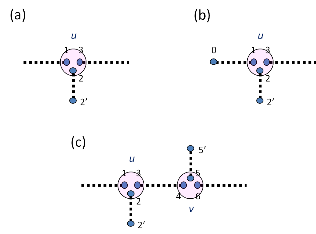
Suppose the POVM on one of the center spin-3/2 $u$ results in $a_{u}\in\{x,y,z\}$; see Fig. 3a. As seen from Eq. (7) or the stabilizer operators in Eq. (10), the three virtual qubits at $u$ are projected to the subspace spanned by $|000\rangle$ and $|111\rangle$, with $|0/1\rangle$ being the eigenstates of $\sigma_{a_{u}}$ (and the quantization axis being $a_{u}$). Furthermore, from the discussions above, there is a stabilizer operator for the post-POVM state, as $-\sigma_{a_{u}}^{[2]}\otimes\sigma_{a_{u}}^{[2^{\prime}]}$ commutes with $\tilde{F}_{u,a_{u}}$, where $2$ denotes the virtual spin-1/2 on site $u$ that connects $2^{\prime}$. Thus, the only two possibilities of the joint state of $u$ and the connected qubit $2^{\prime}$ can be only $|(000)_{u}1_{2^{\prime}}\rangle$ and $|(111)_{u}0_{2^{\prime}}\rangle$, as they satisfy

This means that the two physical spins $u$ and $2^{\prime}$ constitute the encoding of an effective qubit.

Now that we have identified the encoding of a qubit, we would like to seek the encoding of Pauli X and Z operators. Let us suppose $a_{u}=z$ and thus the two states $|\overline{0}\rangle\equiv|(000)_{u}1_{2^{\prime}}\rangle$ and $|\overline{1}\rangle\equiv|(111)_{u}0_{2^{\prime}}\rangle$ (with the basis $|0/1\rangle$ such that $\sigma_{z}|0/1\rangle=\pm|0/1\rangle$) constitute the basis states of a logical qubit. There are four equivalent choices of Pauli $Z$: (1) $\sigma_{z}^{[1]}$, (2) $\sigma_{z}^{[2]}$, (3) $\sigma_{z}^{[3]}$ and (4) $-\sigma_{z}^{[2^{\prime}]}$, as these satisfy that $Z|\overline{0}\rangle=|\overline{0}\rangle$ and $Z|\overline{1}\rangle=|\overline{1}\rangle$. The four choices are equivalent, as any two of them are connected by a stabilizer operator, e.g., $\sigma_{z}^{[2]}=\sigma_{z}^{[1]}(\sigma_{z}^{[1]}\otimes\sigma_{z}^{[2]})$. To obtain the effective Pauli X, which has action that takes $|\overline{0}\rangle$ to $|\overline{1}\rangle$ and vice versa, we can check the following combination works,

On the other, when $a_{u}=x$, the two basis states are $|\overline{0}\rangle\equiv|(+++)_{u}(-)_{2^{\prime}}\rangle$ and $|\overline{1}\rangle\equiv|(---)_{u}(+)_{2^{\prime}}\rangle$, where $\sigma_{x}|\pm\rangle=\pm|\pm\rangle$. The four equivalent choices of effective Pauli $Z$ are: (1) $\sigma_{x}^{[1]}$, (2) $\sigma_{x}^{[2]}$, (3) $\sigma_{x}^{[3]}$ and (4) $-\sigma_{x}^{[2^{\prime}]}$, as these satisfy that $Z|\overline{0}\rangle=|\overline{0}\rangle$ and $Z|\overline{1}\rangle=|\overline{1}\rangle$. The effective Pauli X can be chosen to be

as $X|\overline{0}\rangle=|\overline{1}\rangle$ and $X|\overline{1}\rangle=|\overline{0}\rangle$. Effectively, the POVM outcome $a_{u}$ indicates the new quantization axis for the effective qubit. For a summary of stabilizer generators, effective Pauli $X$ and $Z$ operators, please refer to Table 1, which also includes the case of $a_{u}=y$ outcome.

As exemplified in Fig. 3b, if the center spin-3/2 is located at either end, it has two virtual spin-1/2’s connected to it. The three sites form the basis of the qubit encoding: $|(000)_{u}1_{0}1_{2^{\prime}}\rangle$ and $|(111)_{u}0_{0}0_{2^{\prime}}\rangle$.

Now suppose the POVM’s on several consecutive sites of center spin-3/2 result in a same outcome; see the example in Fig. 3c for two sites with $a=a_{u}=a_{v}$. Those spin-3/2’s and the connected virtual spin-1/2’s together form the encoding of a logical qubit. This is due to additionally that there is a stabilizer operator $-\sigma_{a}^{[3]}\otimes\sigma_{a}^{[4]}$ for the virtual qubits on the two of the neighboring center sites $u$ and $v$ with the same POVM outcome $a$ and that $-\sigma_{a}^{[3]}\otimes\sigma_{a}^{[4]}$ commutes with both $\tilde{F}_{u,a}$ and $\tilde{F}_{v,a}$. Therefore, the two blocks that consists of two spin-3/2’s ($u$ and $v$) and two spin-1/2’s ($2^{\prime}$ and $5^{\prime}$) altogether only encode one qubit with two basis states being $|(000)_{u}1_{2^{\prime}}(111)_{v}0_{5^{\prime}}\rangle$ and $|(111)_{u}0_{2^{\prime}}(000)_{v}1_{5^{\prime}}\rangle$. This result generalizes to any number of consecutive center sites having the same POVM outcome [14]. When all spin-3/2 sites along a chain has been performed of POVM, there is a sequence of POVM outcomes, e.g., $xxyzxzzzy\cdots.$ Consecutive sites of the same outcome (e.g., $xx$ and $zzz$) are grouped into what we call a domain.

We remark that by single-spin measurements, the encoding of a logical qubit by a domain can be reduced to a single site. For example, if one measures the spin at site $v$ in the basis $|\pm\rangle\equiv(|0\rangle\pm|1\rangle)/\sqrt{2}$, a state $\alpha|(000)_{u}1_{v}\rangle+\beta|(111)_{u}0_{v}\rangle$ will be reduced to $\alpha|(000)_{u}\rangle\pm\beta|(111)_{u}\rangle$, depending on the outcome of the measurement. Similarly, if one measures the spin at site $u$ in the basis $(|000\rangle\pm|111\rangle)/\sqrt{2}$, which is, in terms of spin-3/2 language, $(|+3/2\rangle\pm|-3/2\rangle)/\sqrt{2}$, the post-measurement state becomes $\alpha|0_{v}\rangle\pm\beta|1_{v}\rangle$. Thus, an encoded cluster state can thus be reduced by local measurement to a cluster state, where each site is effectively a qubit. For simplicity, from now on we shall focus on cases where no neighboring sites sharing the same outcome for illustration.

To show that the post-POVM CMDB state is an (encoded) cluster state, let us take the example shown in Fig. 4. Let us labels the three center sites in blocks $U$, $V$ and $W$ by the lower-case symbols $u$, $v$ and $w$ respectively. Suppose the POVM outcomes on these sites are $a_{u}=x$, $a_{v}=z$, and $a_{w}=x$, respectively. First note that $-\sigma_{x}^{[3]}\sigma_{x}^{[4]}$ commutes with $\tilde{F}_{u,x}$ and $-\sigma_{x}^{[6]}\sigma_{x}^{[7]}$ commutes with $\tilde{F}_{u,x}$. Note also that $-\sigma_{x}^{[5]}\sigma_{x}^{[5^{\prime}]}$ is a stabilizer operator of the singlet between $5$ and $5^{\prime}$, but it does not commute with $\tilde{F}_{v,z}$. However, if we multiply all the above operators, we obtain

Because $K_{V}$ commutes with $\tilde{F}_{v,z}$, due to the identity

it is a stabilizer operator of the post-measurement state. In terms of logical Pauli operators ${Z}_{U}\equiv\sigma_{x}^{[3]}$ , ${Z}_{W}\equiv\sigma_{x}^{[7]}$, ${X}_{V}\equiv\sigma_{x}^{[4]}\sigma_{x}^{[5]}\sigma_{x}^{[6]}\sigma_{x}^{[5^{\prime}]}$ (see the examples given in the previous section for the effective Pauli operators), we arrive at the stabilizer operator $K_{V}=-{Z}_{U}{X}_{V}{Z}_{W}$. This is (up to a sign) the stabilizer operator defining a linear cluster state [4]. We note that for completeness of the qubit encoding for blocks $U$, $V$ and $W$, the corresponding conjugate operators $Z$ or $X$ can be chosen as follows: ${X}_{U}\equiv\sigma_{z}^{[3]}$, ${X}_{W}\equiv\sigma_{z}^{[7]}$ and ${Z}_{V}\equiv\sigma_{z}^{[4]}$ and that they satisfy the required anticommutation with their conjugate operators.

Note that the choice of three consecutive sites (or domains) is arbitrary. Furthermore, if the above example is changed to a four-site problem, e.g., with the POVM outcomes being $xzzx$, i.e., with middle two sites having the same $z$ outcome. These two sites form a single logical qubit, as discussed earlier in Sec. IV.2, and the encoded Pauli $X$ operators will span across the two sites. The above example can be straightforwardly generalized to a general proof that the state after the POVM is, under local unitary transformation, equivalent to an encoded cluster state, similar to the case of 2D AKLT state on the honeycomb lattice [14]. (The encoding of logical qubits can be reduced to single sites by suitable local measurements, as remarked earlier.) As a further illustration, let us consider another example of three sites in Fig. 4 but with $a_{u}=x$, $a_{v}=z$, and $a_{w}=y$, i.e., the last site has a different outcome $a_{w}=y$ than the above example. Because of this, one now considers $-\sigma_{y}^{[6]}\sigma_{y}^{[7]}$ instead of $-\sigma_{x}^{[6]}\sigma_{x}^{[7]}$ and can show that the follow operator is a stabilizer generator:

Now, one can choose ${Z}_{W}\equiv\sigma_{y}^{[7]}$, ${Z}_{U}\equiv\sigma_{x}^{[3]}$ , ${Z}_{W}\equiv\sigma_{y}^{[7]}$, ${X}_{V}\equiv\sigma_{x}^{[4]}\sigma_{x}^{[5]}\sigma_{x}^{[6]}\sigma_{x}^{[5^{\prime}]}$, and $Z_{V}\equiv\sigma_{z}^{[6]}$ (see Table 1) and obtain

Although the stabilizer operator $K_{V}$ is not of the canonical form of the cluster-state stabilizer ${Z}_{U}{X}_{V}{Z}_{W}$ , they are related by local unitary transformation that leaves $Z_{V}$ invariant.

The hidden cluster state in the ground state of the AKLT quasichain is hence revealed by the POVM (5) or equivalently (6). The original 1D spin-1 AKLT state has previously been shown to be locally converted to a 1D cluster state by a similar spin-1 POVM [14] and by a different alternating POVM [21].

In the case of a disconnecter, the two virtual spin-1/2 particles (of the single spin $B$) are each applied an effective Pauli X gate $X=|0\rangle_{a}\langle 1|+|1\rangle_{a}\langle 0|$ [22] before being measured in the basis of respective $|\pm\rangle_{a}$, where the axis label $a$ can be either $x$, $y$, or $z$ (depending on the POVM outcome on the neighboring spin-3/2 particle) and $|\pm\rangle_{a}\equiv(|0\rangle_{a}\pm|1\rangle_{a})/\sqrt{2}$ with $\sigma_{a}|0/1\rangle_{a}=\pm|0/1\rangle_{a}$; see Fig. 5. Suppose the outcome of the measurement on the spin-1/2 connected to the spin-3/2 $u$ is labeled by $(-1)^{m_{1}}$ with $m_{1}=0/1$, and similarly for the one connected to $v$: $(-1)^{m_{2}}$. (Together, $m_{1}$ and $m_{2}$ characterize the measurement outcome of the merged spin-3/2 $B$.) Then the effect of measuring the spin $B$ on neighboring $u$ and $v$ is that single-qubit gates $Z_{u}^{m_{1}}\otimes Z_{v}^{m_{2}}$ have been applied to $u$ and $v$, where $Z_{u}=|3/2\rangle_{a_{u}}\langle 3/2|-|-3/2\rangle_{a_{u}}\langle-3/2|$ and similarly for $Z_{v}$. Note that in the three-virtual-qubit picture, $|+3/2\rangle_{a_{u}}=|000\rangle_{a_{u}}$ and $|-3/2\rangle_{a_{u}}=|111\rangle_{a_{u}}$. Furthermore, the measurement on 1 and 2 corresponds to a local measurement on the spin-3/2 $B$. The logical qubits on neighboring chains evolve independently, i.e., no entangling gate has been applied to $u$ and $v$.

In the case of a connecter, the two spin-1/2 particles are first applied effective Pauli X gates: $X=|0\rangle_{a}\langle 1|+|1\rangle_{a}\langle 0|$ and then a control-phase (CP) gate: ${\rm CP}_{12}=|0\rangle_{{a_{u}}}\langle 0|^{[1]}\otimes\openone^{[2]}+|1\rangle_{a_{u}}\langle 1|^{[1]}\otimes Z_{a_{v}}^{[2]}$, where $Z_{a_{v}}=|0\rangle_{a_{v}}\langle 0|-|1\rangle_{a_{v}}\langle 1|$. These operations correspond a single-spin unitary transformation on the merged $B$ spin. Then, a measurement in their respective $|\pm\rangle_{a}$ basis is made as in the previous case, and the effect is that an entangling gate has acted on the two associated spin-3/2 particles $u$ and $v$ (which are effectively two qubits), up to Pauli gates. Using the measurement labels $m_{1}$ and $m_{2}$, the entangling gate that has been applied is $Z_{u}^{m_{1}}\otimes Z_{v}^{m_{2}}\,{\rm CP}_{uv}$, where

where $I^{[v]}_{a_{v}}=|3/2\rangle_{a_{v}}\langle 3/2|+|-3/2\rangle_{a_{v}}\langle-3/2|$ is the effective qubit identity operator and $Z_{a_{v}}=|3/2\rangle_{a_{v}}\langle 3/2|-|-3/2\rangle_{a_{v}}\langle-3/2|$ is the effective Pauli Z operator. The logical qubits on neighboring chains have thus undergone a control-phase gate up to Pauli Z’s.

We remark that the approach of the joint measurement on the two virtual qubits has also been used recently in Refs. [13] and [23] and was employed earlier in Ref. [24]. In summary, an entangling gate can indeed be applied on two logical qubits residing on the two neighboring quasichains. Thus, we see that CMDB state is a universal resource for MBQC.

The whole system can be further converted to a 2D cluster state on a honeycomb lattice. First, a structure which is topologically equivalent to a honeycomb (or brick-wall) lattice can be identified. Second, by suitable disconnecting or connecting measurements on $B$ sites and then Pauli measurements on $A$ sites, the structure can be reduced to a honeycomb lattice. Shown in Fig. 6 is the example of five quasichains. In Fig. 6a, the shaded boxes enclose sites that share the same POVM outcomes on $A$ sites. The $B$ sites are not shown explicitly and only vertical dashed lines are used to indicate the possible connecter/disconnecter roles by $B$ spins. In Fig. 6b, the solid vertical lines denote the choice of a connecter (and the remaining dashed vertical lines in Fig. 6a denote disconnecters) and hence a control-phase gate acts on two neighboring $A$ sites connected by solid vertical lines. The dangling spin-1/2’s sites are omitted. Those boxes with a ‘Y’ represent a subsequent Pauli-Y measurement to remove the qubit on the sites and to link its two neighboring blocks, resulting in a graph state that has the brickwall structure, as shown in Fig. 6c. This illustrates and generalizes to a proof that a 2D cluster state can be distilled from the CMDB state.

References

- [1] M. Nielsen and I. Chuang, Quantum Computation and Quantum Information (Cambridge Univ. Press, 2000).
- [2] R. Raussendorf and H. J. Briegel, Phys. Rev. Lett. 86, 5188 (2001).
- [3] H. J. Briegel, D. E. Browne, W. Dür, R. Raussendorf, and M. Van den Nest, Nature Phys. 5, 19 (2009).
- [4] H. J. Briegel and R. Raussendorf, Phys. Rev. Lett. 86, 910 (2001).
- [5] M. Hein, J. Eisert, and H.-J. Briegel, Phys. Rev. A 69, 062311 (2004).
- [6] M. Van den Nest, A. Miyake, W. Dür, and H. J. Briegel, Phys. Rev. Lett. 97, 150504 (2006).
- [7] D. Gross, S. T. Flammia, and J. Eisert, Phys. Rev. Lett. 102, 190501 (2009); M. Bremner, C. Mora, and A. Winter, ibid 102, 190502 (2009).
- [8] D. Gross and J. Eisert, Phys. Rev. Lett. 98, 220503 (2007); D. Gross, J. Eisert, N. Schuch, and D. Perez-Garcia, Phys. Rev. A 76, 052315 (2007); D. Gross and J. Eisert, Phys. Rev. A 82, 040303(R) (2010).
- [9] F. Verstraete and J. I. Cirac, Phys. Rev. A 70 060302(R) (2004).
- [10] Measurement-based quantum computation with these new resource states take place in the so-called “correlation space” rather than the Hilbert space of physical qubits; see Ref. [8].
- [11] S. D. Bartlett and T. Rudolph, Phys. Rev. A 74, 040302(R) (2006).
- [12] X. Chen, B. Zeng, Z.-C. Gu, B. Yoshida, and I. L. Chuang, Phys. Rev. Lett. 102, 220501 (2009).
- [13] J.-M. Cai, A. Miyake, W. Dür, and H. J. Briegel, Phys. Rev. A 82, 052309 (2010).
- [14] T.-C. Wei, I. Affleck, and R. Raussendorf, Phys. Rev. Lett. 106, 070501 (2011); T.-C. Wei, I. Affleck, and R. Raussendorf, e-print arXiv:1009.2840.
- [15] A. Miyake, Ann. Phys. (Leipzig) 326, 1656 (2011).
- [16] M. A. Nielsen, Rep. Math. Phys. 57, 147 (2005).
- [17] I. Affleck, T. Kennedy, E. H. Lieb, and H. Tasaki, Phys. Rev. Lett. 59, 799 (1987); I. Affleck, T. Kennedy, E. H. Lieb, and H. Tasaki, Comm. Math. Phys. 115, 477 (1988).
- [18] G. K. Brennen and A. Miyake, Phys. Rev. Lett. 101, 010502 (2008).
- [19] D. Gottesman, Stabilizer Codes and Quantum Error Correction, Ph.D. Thesis, Caltech (1997).
- [20] Stabilizer operators in the stabilizer are unitary operators that commute with one another. is a stabilizer operator of the state if it satisfies . One important property of qubit stabilizer operators is that when the number of independent stabilizer operators equals that of the total number of qubits in , the state is uniquely determined. If there is one independent stabilizer less, then the state is only determined up to a subspace of an effective qubit. For details, see Ref. [19].
- [21] X. Chen, R. Duan, Z. Ji, and B. Zeng, Phys. Rev. Lett. 105, 020502 (2010).
- [22] The reason to apply a Pauli X is to flip the encoding states of the and its assocaite particles from and [see Eq. (11)] to and , respectively, is for convenience of later analysis. One then investigates the effect on and due to the measurement on the associated and in the basis. In the case of a connecter, an additional control-phase gate is applied to and before measurement.
- [23] Y. Li, D. E. Browne, L. C. Kwek, R. Raussendorf, and T.-C. Wei, Phys. Rev. Lett. 107, 060501 (2011).
- [24] D. Gottesman and I. Chuang, Nature 402, 390 (1999).
- [25] M. Van den Nest, W. Dür, A. Miyake, and H. J. Briegel, New J. Phys. 9, 204 (2007).
- [26] J.-M. Cai, W. Dür, M. Van den Nest, A. Miyake, and H. J. Briegel, Phys. Rev. Lett. 103, 050503 (2009).