Non-standard antineutrino interactions at Daya Bay
Abstract
We study the prospects of pinning down the effects of non-standard antineutrino interactions in the source and in the detector at the Daya Bay neutrino facility. It is well known that if the non-standard interactions in the detection process are of the same type as those in the production, their net effect can be subsumed into a mere shift in the measured value of the leptonic mixing angle . Relaxing this assumption, the ratio of the antineutrino spectra measured by the Daya Bay far and near detectors is distorted in a characteristic way, and good fits based on the standard oscillation hypothesis are no longer viable. We show that, under certain conditions, three years of Daya Bay running can be sufficient to provide a clear hint of non-standard neutrino physics.
I Introduction
The past and ongoing neutrino oscillation experiments provide a firm evidence that the neutrino flavour is changing throughout the neutrino propagation. Except for some recent signals reported by MINOS [1] and MiniBooNE [2] (and also previously by LSND [3]) the vast majority of the data is consistent with the hypothesis of neutrino flavour oscillations driven by a pair of mass-squared differences: (or if an inverse neutrino mass hierarchy is realized), often called the atmospheric mass-squared difference, and the solar mass-squared difference , together with a pair of the corresponding mixing angles: (or the inverse hierarchy case) and [4]. This, however, requires at least two of the oscillating neutrinos to be massive.
By construction, neutrinos are massless in the Standard Model (SM). Thus, a lot of effort has been spent on devising SM extensions that could not only accommodate the unprecedented smallness of the light neutrino mass scale and all the peculiarities of the leptonic mixing pattern, but also provide specific new physics signals, thus admitting for a further experimental scrutiny. In some cases, such new physics effects could even be expected to be within the reach of near future experimental facilities. In this respect, the seesaw approach [8, 12, 6, 9, 11, 7, 10, 5], in which the smallness of the absolute neutrino mass scale is usually linked to a very specific type of high energy dynamics, represents a particularly plausible model-building paradigm.
Each dynamical realization of the seesaw picture makes some kind of new physics effects appear, at least at a certain level. This, in turn, makes the neutrino sector an ideal probe to physics beyond the SM. For instance, the Majorana nature of the light neutrinos inherent to the seesaw framework provides characteristic lepton-number-violating signals at low energies like, e.g., the neutrinoless double beta decay, or, if kinematically accessible, same-sign di-lepton production at colliders, see, e.g., [13]. Similarly, besides neutrino oscillations, the flavour structure of the lepton sector can be tested in lepton-flavour-violating processes such as or, for example, trilepton collider events, c.f., [14].
A full exploration of such new physics signals generally requires a very good knowledge of the leptonic flavour mixing angles governing the neutrino oscillation phenomena. In particular, the smallest mixing angle , which plays a central role in the leptonic CP violation, is still to be determined (with a current C.L. upper bound of reported by the CHOOZ collaboration [15] and first indications of its non-zero value obtained by T2K [16] and MINOS [17] experiments).
The Daya Bay neutrino oscillation experiment [18] is designed to perform a precision determination of with a potential to improve the CHOOZ limit by one order of magnitude. More specifically, the -sensitivity of Daya Bay is anticipated to reach 0.01 at confidence level over the entire allowed range of , see Fig. 3.12. in [18]. At the assumed best fit point the expected sensitivity is around 0.008 with 3 years of data. Such a highly ambitious goal relies on a very good control over the systematics, which is achieved by employing a unique set of eight identical detectors deployed at three different locations optimized for monitoring the antineutrino rates from the six reactors. A similar experimental setup is also adopted by the upcoming Double Chooz experiment [19] and RENO [20] experiments.
In combination with the large statistics due to the huge flux of antineutrinos produced in the nearby nuclear reactors, the unprecedented accuracy of this new generation of reactor experiments can make them sensitive to the new physics effects, at least at a certain level. For instance, if the new physics sector couples to hadrons and the relevant scale is not very high, one can expect non-standard interactions (NSI’s) in the antineutrino production and detection processes as well as non-standard matter effects the antineutrinos experience throughout the propagation process. Similarly, new neutral fermions can mix with the three SM active neutrinos, which would result in an effective non-unitarity of the leptonic mixing matrix entering the relevant oscillations probabilities.
The NSI’s in reactor neutrino experiments have been discussed previously in, e.g., [21, 22], especially when the production and detection processes (and the corresponding non-standard effects) are assumed to be just inverse of each other. In particular, it has been shown that in such a case the NSI effects can be subsumed into a mere shift in the measured value of the effective mixing angle .
In this work, we study the NSI’s in reactor antineutrino experiments in a general case when the assumption that the source and at the detector processes including the non-standard effects are just inverse of each other is dropped. This, in turn, leads to a specific distortion in the ratio of the antineutrino spectra measured in the far and in the near detectors which can not be entirely transformed away by mere shifts in the relevant oscillation parameters, i.e., and . We show that, under certain conditions, three years of Daya Bay running can be sufficient to provide a clear hint of non-standard neutrino physics.
The remainder of the manuscript is organized as follows: In Sec. II, we present the general formalism and derive the relevant antineutrino survival probability formulas used in the subsequent analysis. Two basic scenarios corresponding to qualitatively different shapes of NSI’s are specified in Sect. III, and a detailed analysis of the observability of such effects at Daya Bay is performed in Sect. IV. Finally, we conclude in Sect. V.
II Non-standard interactions in reactor antineutrino oscillations
II.1 Non-standard interactions in the antineutrino sources and detectors
In what follows, we adopt the standard SPD (source, propagation, and detector) approach [23] to consider the antineutrino oscillation process in a reactor antineutrino experiment. In the presence of NSI’s, the antineutrino states produced in the source as well as those observed in the detector can be treated as superpositions of pure orthonormal flavour states
| (1) |
where the superscripts ‘’ and ‘’ denote the source and the detector, respectively. Note that there is no need to include the appropriate normalization factors in expressions (1) because we are going to be interested only in ratios of the survival probabilities in the near and far detectors where such factors cancel.
The current experimental bounds on the NSI parameters mainly come from the lepton flavour violating decays , the universality test of weak interactions and the invisible decay width of the -boson. Model-independent studies indicate that the upper limits on the NSI parameters are typically in the ballpark of to , see e.g. [24] and references therein.
To keep the analysis as general as possible, in what follows we shall consider two basic physical situations, namely, (to be called case I, cf. Section III.1) and also (case II, see Section III.2) and provide a detailed performance analysis of the Daya Bay experimental setting in each case.
Few comments are worth here: First, it is not very common to assume as, in such a case, given the inverse microscopic nature of the relevant source and detection processes in standard reactor neutrino experiments, one usually concludes that these two quantities should be equal, see e.g. [21]. This, however, is based on several implicit assumptions, in particular: 1) exact CPT (and Lorentz) invariance and 2) factorizability of the source, propagation and detection processes. As for the former, CPT violation (implying also the Lorentz invariance breakdown), for instance, makes it possible to have masses and mixings different for neutrinos and antineutrinos. Hence, the mixing matrix entering the detection process can be different from the one governing the antineutrino production and, thus, the standard oscillation formula is not valid even if all the NSI parameters are set to zero. Nevertheless, at least to the leading order in and , such an effect can be still accounted for within the standard SPD formalism by a suitable redefinition of the NSI parameters, thus generating an effective departure from the assumed case, cf. formula (8) in Section II.3. An interested reader can find further comments in, e.g., the recent work [25] and references therein. Needless to say, these considerations became especially relevant with the recent claims of observation of possibly superluminal neutrinos in the OPERA experiment [26]. Concerning 2), it is clear that as long as the antineutrino is produced in the source by the classical SM charged current interaction no departure from the basic case I setting can be expected because all the flavour-blind standard nuclear effects such as, e.g., the enhancement of scalar and/or tensor modes etc., simply factorize out and, hence, contribute only to the change of normalization of the total neutrino fluxes. In this respect, the case can be viewed as a model-independent parametrization of non-factorizable flavour-dependent new physics effects which, at low energies, can correspond to higher-dimensional terms in the effective lagrangian such as, e.g., (which can be relevant also to other processes such as neutron star cooling, see, e.g., [27]) etc. Therefore, though possibly marginal from the perspective of the conventional extensions of the SM, we still find this setting worth a closer look, the more that Daya Bay can perform very well in this case, see Sections IV.4.2 and IV.4.3.
II.2 Non-standard interactions in the antineutrino propagation
The propagation of antineutrino flavour eigenstates from the sources to the detectors is governed by the effective Hamiltonian
| (2) |
where is a Hermitian matrix parametrizing the NSI’s throughout the antineutrino propagation and arises due to effects of the coherent forward scattering in matter (with denoting the electron number density along the antineutrino trajectory). Barring the irrelevant Majorana phases, the vacuum leptonic mixing matrix is conveniently parametrized by three mixing angles , and and one Dirac CP phase [28]
| (3) |
with and (for , and ). The full effective Hamiltonian (2) is diagonalized via a unitary transformation
| (4) |
where () denote the effective masses of neutrinos and is the effective leptonic mixing matrix in matter.
The size of the matter effect driven by the term amounts to around eV2/MeV for Earth crust with density of 2.8 g/cm3. Even for the highest values of reactor antineutrino energies of around 10 MeV, this number is about 40 times smaller than the value of eV2/MeV and about 1100 times smaller than eV2/MeV. This indicates that Earth matter effects are very small and can be safely neglected. Hence, we take or, equivalently, set in Eq. (2).
II.3 The antineutrino survival probability
With the NSI effects at play, the electron antineutrino survival probability amplitude is given by
| (5) |
where is the propagation distance and is a coherent sum over the contributions of all the mass eigenstates
| (6) |
The antineutrino survival probability is then given by . For completeness, let us remark that a corresponding neutrino oscillation amplitude can be readily obtained from (5) with a substitution . It should also be stressed that only the first row of and the first column of are relevant to the -type transition amplitude. Namely, the NSI parameters and involved in reactor neutrino experiment contain at least one flavour index .
Inserting formula (6) into Eq. (5) one arrives at the full antineutrino oscillation probability
| (7) |
where , and
| (8) |
In the limit, Eq. (7) reduces to the standard survival probability.
In this study, the quantity of our main interest is the third term in Eq. (7) which, being linear in the sine of , does not play any role in the standard oscillation case. In this respect, a potential deviation from the “standard” quadratic-sine dependence in an oscillation experiment can be interpreted as a hint of non-standard antineutrino interactions, in particular if such an anomaly exhibits the characteristic linear-sine shape.
II.4 Series expansion of the antineutrino survival probability
In practice, given the finite precision of the experimental inputs, it is very convenient to expand the survival probability (7) around the standard oscillation formula in terms of the relevant small parameters, in particular which are all expected to be at most at the few per-cent level, c.f. [24] and references therein. In addition, is small compared to the other mixing angles (with the current CHOOZ upper limit of ) and, hence, it amounts to another useful expansion parameter. Moreover, for the Daya Bay far detector, also the oscillation term turns out to be at the level of to and, as such, it can also be viewed as a small quantity.
Taking all this into account, we obtain the following expanded form of the relevant electron antineutrino survival probability
| (9) | |||||
where corresponds to the standard oscillation probability, i.e., the one without NSI’s which is approximately given by
| (10) |
Inspecting Eq. (9) one can recognize three qualitatively different non-standard contributions to : In the first two lines there is a CP-even term quadratic in sine of which, as expected, may affect the determination of the mixing angle . The remaining three lines denote the CP-odd NSI effects corresponding to two different kinematical regimes characterized by and , respectively. Notice that in the standard parametrization (3), the Dirac CP-violating phase groups only with the former factor. It is also worth noticing that the term proportional to tends to be further suppressed in the “flavour-blind” setting (with ) because of the proximity of and .
It shall be noted that both the standard and the NSI transition probabilities depend on the neutrino mass hierarchy. For the standard oscillations, the hierarchy-sensitive terms are of the order of and thus can be consistently neglected in Eq. (10). The NSI-dependent terms in Eq. (9), however, contain a term linear in sine of which, indeed, differs in sign in the normal and in the inverted hierarchy schemes, respectively. Since, however, we do not expect any distinctive NSI features to be large enough to discriminate among these two settings (although they would certainly differ in details), in what follows, we shall deliberately stick to the normal hierarchy case, i.e., assume .
II.5 Notation and conventions
In what follows we shall adopt the following parametrization:
| (11) |
where the universal index was dropped for simplicity. It is also convenient to define the source and detector phase averages and differences , respectively:
| (12) |
The latter has a clear physical meaning: indeed, for all (together with ) one recovers a limit in which the non-standard antineutrino interactions in the detection process are of the same kind as those in the production.
III Specific settings
In what follows, we shall discuss two simple but phenomenologically interesting shapes of NSI’s and discuss the relevant effects in the reactor antineutrino experiments.
III.1 Case I:
We start with the simplest case characterized by the assumption which corresponds to the situation where the production and the detection processes (including the associated non-standard interactions) are just inverse of each other. The relevant antineutrino survival probability (9) is then reduced to
| (13) | |||||
Remarkably, the linear sine-dependent term in Eq. (9) vanishes and the NSI effects enter the survival probability as a mere global shift of the oscillation amplitude. This amounts to a shift in the “effective” reactor mixing angle
| (14) | |||||
Namely, the oscillation probability is given by the standard formula (10) with replaced by the effective mixing angle . Thus, there is no way to discriminate such an NSI effect from standard oscillations in reactor antineutrino experiments. It is also worth noting that the CP phase differences enter Eq. (14) via cosines only which is, indeed, justified by the CP properties of the survival probability in the setting under consideration.
In Fig. 1, we display the standard and the modified oscillation probability in the NSI presence as a function of the antineutrino energy in a detector at the “ideal” distance km (optimized for the highest count rate at MeV) from the source.

The ‘‘depth’’ of the first oscillation minimum (the solid line for the standard oscillations) changes significantly if the NSI effects are turned on (dashed line); however, the energy of the minimum determined by the neutrino mass-squared differences remains essentially unchanged.11 1 Let us remark that the energies corresponding to the two relevant minima are not exactly the same due to the presence of the sub-leading terms proportional to in Eqs. (9) and (10).
Nevertheless, though the reactor antineutrino experiments in this case cannot distinguish the NSI’s from a true mixing angle on their own, they can still provide a useful piece of information in combination with other types of experiments such as, e.g., accelerator experiments, superbeams, beta-beams, neutrino factories, etc. In particular, if these searches report different values of , NSI’s could be responsible for the mismatch.
III.2 Case II:
As already mentioned in Section II.1, we do not intend to confine ourselves entirely to the “canonical” case with , but rather prefer to keep the mind open also to the intriguing possibility. Indeed, the distortion of the shape of the detected antineutrino spectra with respect to the standard oscillation picture expected with such a choice of the NSI parameters in the effective quantum-mechanical SPD picture can mimic (at the leading order) a wide class of new physics effects such as, e.g., a net CPT violation or, for instance, non-factorizable beyond-Standard-Model effects in the production processes, cf. Section II.
As a consequence, the terms linear in sine in formula (9) are exposed and the relevant NSI effects can no longer be completely subsumed into a shift of the effective mixing angle . This, besides the change of the “depth” of the first oscillation minimum (c.f. Figure 1), leads also to a shift in its energy, as illustrated in Figure 2.

In particular, the dip can be shifted by as much as one in both directions, depending on the specific choice of the NSI parameters.
In what follows we shall focus on two specific realizations of this setting, namely, the case when the magnitude of the NSI parameters differs between the production and detection processes (Case IIa) and the case when the relevant NSI parameters are of the same size but differ by their phases (Case IIb). Both these cases are studied numerically in Sect. IV.
III.2.1 Case IIa: Non-standard interactions in source only
Let us exemplify the first option on a specific setting where the NSI’s exhibit themselves only in the production processes, i.e., taking . Given that, the general formula (9) simplifies into
| (15) | |||||
where we used and . It is worth noting that the genuine NSI effect (due to the last two terms) is proportional to sines of differences of the Dirac CP phase and the CP phases of the NSI parameters , as expected for a CP-violating effect beyond the standard oscillation picture.
III.2.2 Case IIb: Same-size source and detector effects with different phases: ,
An interesting complementary setting is obtained if the magnitude of the source and detector effects are assumed to be equal so that the NSI effects can only be distinguished due to the mismatch between the corresponding CP phases and . With , the general formula (9) receives a rather symmetric form22 2 Note that the coefficient of the last term in Eq. (16) is optically different from the same in Eq. (9) which is due to the utilized goniometric identity for a difference of two sines and the definition of .
| (16) | |||||
where the notation specified in Eq. (12) has been used. Again, the relevant phase differences in the genuine NSI terms enter in sines. Furthermore, the formula above can be simplified to a yet more compact form
| (17) | |||||
which does expose the “kinematic” role of the phase differences and the “amplitude modulation” role of their averages .
Let us also remark that for (when the symmetric setting with is recovered) the last term vanishes and, as expected, the other terms conspire to yield a mere shift in the effective mixing angle identical to that given in formula (14). This provides a nice consistency check of the results. A simple numerical analysis of both Case-IIa and Case-IIb settings is given in Sect. IV.
IV Non-standard antineutrino interactions at Daya Bay
IV.1 Experimental setting
The Daya Bay neutrino experiment [18] is designed to perform a precision measurement of using antineutrinos produced by the reactors of the Daya Bay Nuclear Power Plant (NPP) and the Ling Ao NPP. In the detectors, antineutrinos from the reactors are captured via the inverse beta-decay process, and the deficit from the expected dependence is to be interpreted as a signature of neutrino oscillations. In particular, near and far detectors are employed in order to suppress the systematic uncertainties related to the antineutrino flux from the reactors.
The Daya Bay measurement of is expected to reach the sensitivity of the order of , an order of magnitude better than the current CHOOZ limit . Besides a high-quality determination of the relevant standard neutrino oscillation parameters, Daya Bay can be rather efficient in improving some of the current constraints on physics beyond the SM.
In order to estimate the NSI effects possibly observable at Daya Bay, we perform a basic numerical analysis making use of a simple model of the detected neutrino spectra. There are three pairs of nuclear reactor cores of a total thermal power of 17.4 GW at the experiment site, namely, Daya Bay (DYB), Ling Ao (LA) and Ling Ao II (LAII), providing electron antineutrinos to three detectors, two near ones called Daya Bay (DYB) and Ling Ao (LA) with 40 tons and a far detector (FAR) with 80 tons of a Gadolinium-doped liquid scintillator, respectively. A more detailed breakdown of the relevant Daya Bay parameters can be found in TABLE 1.
| DYB layout | geometry | expected daily event rates | |||
|---|---|---|---|---|---|
| DetectorsCores | DYB 22.9 GW | LA 22.9 GW | LAII 22.9 GW | mods.DR [18] | simulated |
| DYB (40 t) | 363 | 1347 | 1985 | ||
| LA (40 t) | 857 | 481 | 1618 | ||
| FAR (80 t) | 1307 | 526 | 1613 | ||
IV.2 A simple model of the spectra
For the sake of simplicity, we shall assume that each pair of neighboring cores constitute a single point source. The average energy release per one fission is anticipated to be around 200 MeV [18] so the estimated number of fissions per second in each reactor site is
| (18) |
where the extra factor 2 counts the number of reactor cores per site and stands for the thermal power of each core. For the spectrum of the antineutrino flux per fission we shall use the approximate formula given in Ref. [29] (for in MeV):
| (19) |
Antineutrinos interact with the free protons in the scintillator via the inverse beta decay process . The cross-section of this reaction has been calculated in Ref. [30] to be
| (20) |
with the energy threshold MeV. There are free protons in a cm3 of the scintillator of density g/cm3 [31]. Therefore the number of targets per one ton of the scintillator is ton-1.
The antineutrino survival probability is a function of energy, propagation distance, oscillation parameters and, in general, also the NSI parameters. The expected total number of antineutrino events in the detector (with DYB,LA,FAR) with mass after three years of running can be estimated as
| (21) |
where s is the duration of a three-years’ run. We sum over three reactor sites and use for the distance between the detector and the reactor site , c.f. TABLE 1. In addition, we adopt a detection efficiency coefficient [18]. As an example, we depict in Figure 3 the expected spectrum of antineutrinos detected in the DYB detector. It is worth noting that the highest event rate corresponds to .

The quantity of our main interest is the ratio of the antineutrino energy spectra between the considered far and near detectors, which can be obtained readily from Eq. (21). It is expected that, due to a similar design of the far and near detectors, the systematic uncertainties associated to, e.g., the absolute flux determination, can be greatly reduced in the ratio of the energy spectra. However, in order to fully account for all the systematic uncertainties, e.g., the backgrounds, energy miscalibration, detection efficiencies etc., a complex simulation of the Daya Bay experiment is necessary. This, however, is a formidable task in general, so in what follows we shall consider mainly the statistical uncertainties (Sections IV.3 and IV.4) and only later on (in Section IV.5) we demonstrate that the changes due to the (leading-order) systematical effects do not inflict any significant changes on these results.
IV.3 The analysis
To assess the observability of NSI’s at Daya Bay in practice, we perform a simple numerical analysis along the following lines: we choose 15 energy bins from 1.8 MeV to 8 MeV in order to have approximately the same statistics in all bins which are 1-4 times wider than the energy resolution [18]. In each bin, we use Eq. (21) to calculate the ratio of the antineutrino energy spectra between the far and near detectors (for sake of illustration, from now on we shall focus in particular onto the FAR and the DYB detectors). In the case of the standard neutrino oscillations, the expected shape of this ratio between the FAR and the DYB detectors is depicted in Figure 4.

Since the uncertainties of , and are not expected to play any significant role in the ratio of our interest, we shall fix these parameters to their central values. This is not the case of because the uncertainty in this parameter (quantified by ) mimics the effects of the NSI’s, namely, it also shifts the position of the first minimum in . However, with the increasing precision of the determination, these effects become less important. Therefore, in what follows, we shall mainly focus on two specific situation corresponding to different choices of : in one case we take [4] as the current experimental value while in the other “ideal case”, we push down to , respectively (which can be viewed as an optimistic expectation for the uncertainty in the atmospheric mass-squared difference in several years from now).
For each specific choice of the relevant NSI parameters there are only two unknown parameters left in , namely, and , c.f., Eq. (10). Denoting the -th bin value of (as a function of , , and ) by , we attempt to fit the simulated data by the NSI null-hypothesis corresponding to the case when is calculated for standard oscillations with some effective values of the relevant oscillation parameters, namely, . This is done by minimization of the function
| (22) |
with respect to and , where denotes the three-years’ run statistical error(s). The parameter has been left free (to be determined by Daya Bay) whereas should obey the existing experimental constraints. The value of in the minimum () then quantifies the likelihood that the Daya Bay data could be fitted by the standard oscillation formula. For two fitted parameters, and corresponds to and C.L., respectively.
IV.4 Results
For the sake of simplicity, in what follows we shall consider only the “flavourless” versions of the oscillation probability formulas relevant to the three cases of our interest, namely Eqs. (13), (15) and (17). This amounts to setting and everywhere. Let us recall that, besides the standard oscillation parameters, in Case I and Case IIa the relevant input NSI parameters are, namely, the (universal) magnitude of the NSI effects and the corresponding CP phase (more precisely, the phase difference where denotes the leptonic Dirac CP phase) while in Case IIb the NSI parameters entering the survival probability are , (again, it is rather ) and .
Let us also reiterate that only the statistical errors have been taken into account in the current analysis. A complete study including also the systematic uncertainties would require a complex simulation of the Daya Bay experiment. This, however, is beyond the scope of the present study.
IV.4.1 Case I


As we argued in Sect. III.1, in the symmetric setting with , the NSI effects cannot be distinguished from the pure standard oscillations. Even if the underlying mixing angle is zero, one can still fit the data with a standard oscillation curve corresponding to a nonzero value of the effective mixing angle given by formula (14). A pair of representative plots depicting the expected ratio between the FAR and the DYB antineutrino spectra in this situation are given in Figure 5. One can see that the data are well fitted by the standard oscillation formula with just the effective mixing angles different from their “true” values.
IV.4.2 Case IIa
In the “flavourless” setting, the relevant Case-IIa formula (15) simplifies into
| (23) | |||||
where . Note that in most cases the last term can be neglected due to the experimental proximity of to .
We also stress that for or the leading NSI contribution corresponding to the sine-squared term above essentially mimics the effects of standard oscillations with a shifted mixing angle because, besides the last negligible term, there is no net NSI induced CP-violating effect. One can see this on the left panel in Figure 6 where, indeed, the data can be fitted by the standard oscillation formula with just a shifted effective mixing angle .
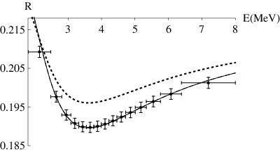

However, the change is still proportional to and thus no shift is induced if the underlying happens to be zero33 3 As we shall see, this is different from the Case IIb setting studied in Sect. IV.4.3 where a nonzero value of the effective mixing angle can be generated even for ..
However, for non-trivial , the NSI effects can no longer be subsumed into a pure shift in and the standard oscillation formula no longer fits the data even if one admits for a certain variation in , see the right panel in Figure 6. Thus, in this case, one can in principle attempt to constrain the and parameters, at least in some parts of their parameter space.
In Figure 7 we present the relevant exclusion regions for these parameters.

Therein, one can observe an interesting -periodicity in , which can be understood from the shape of the second correction in formula (23). Remarkably enough, even with variable and as low as 0.02, in some cases the NSI effects can be distinguished from the standard oscillation at C.L.
IV.4.3 Case IIb
In the more general case when both the source and detector effects are present there is an extra set of parameters at play associated to , i.e., the relevant magnitudes and also the extra detector NSI phases which combine with the source ones into the phase averages and the phase differences , c.f. Eq. (12). As before, we will assume a “flavourless” form of NSI’s and deliberately put in order to simplify the numerical analysis. Then formula (16) reduces to
| (24) | |||||
where, again, . As before, the last term is negligible for close to .
For the sake of illustration, in Figure 8 we show two specific examples of the -fits obtained in Case IIb. There, the data are fitted by the standard oscillations, first with variable and (solid lines) and then also with only as a free parameter (dashed lines).
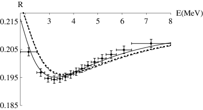

In Figure 9, the exclusion plots for the and parameters are given for and two specific choices of .


The sensitivity in is similar to that observed in Figure 8 for Case IIa. Notice, however, that the two leading corrections in Eq. (16) have a very different -periodicity. The former is -periodic in while the latter is -periodic in . The reason is easily seen from the analytic shape of the relevant survival probability (24). Indeed, for , the second correction in formula (24) dominates over the first one while it is the other way round for .
Regions in the plane where Daya Bay experiment could distinguish non-standard effects from standard oscillations (at and C.L.) are shown in Figure 10 for different values of and .


If the value of the underlying is close to the CHOOZ limit () and then the region is relatively large, see the upper-left panel in Figure 10. With decreasing (from left to right) or (from up to down), the observability domains become naturally smaller.
The possible NSI effects in an independent Daya Bay determination of the standard oscillation parameters and are illustrated in Figure 11. One can see that, at least in some cases, the corresponding global best fit point can differ significantly from the “true” values of these parameters, potentially leading to a tension between Daya Bay and other experiments.

Yet another comment is in order here. As we have seen in Case IIa (c.f., Sect. IV.4.2), with source effects only there is no way to end up with a significant effective if the underlying was zero, while here one still gets even for due to the first term in Eq. (24). Such a qualitative difference in the behavior of these two settings can be heuristically understood as follows: In the former case, there are effectively only two small parameters (with their corresponding CP phases) at play, namely and while there are three such quantities in the latter case, in particular , and . In Case IIa, there is thus only a single relevant phase difference governing the CP-even effects [due to the first correction in Eq. (23)] which, however, becomes ill defined in the limit, and thus its effect can be “rotated away”. Remarkably, this is not so in Case IIb since there is an observable phase difference left even in the limit and the corresponding contribution to the effective due to the first term in Eq. (24) cannot be transformed out.
IV.5 Effects of leading-order systematics
Finally, let us argue that the leading systematical effects do not change the results obtained in the previous sections in any significant way.
The main sources of systematical uncertainties in the Daya Bay setting are related to the reactors (power, spent fuel, location), detectors (energy miscallibration, target mass, detector efficiency) and, of course, backgrounds (accidental signals, 8He 9Li, fast neutrons) [18]. Taking the full advantage of the “near+far” detector setting one can approximate the leading-order systematic uncertainties (namely, the neutrino flux uncertainty and the uncertainty in the detector masses) as a relative change of the measured far-to-near ratio of the detected antineutrino energy spectra , cf. Section IV.3. For the sake of simplicity we shall assume that this change (to be denoted by ), as well as its uncertainty , are energy-independent at the leading order. Following the detailed discussion given in [18] we shall adopt a conservative value of for the calculation.
The argument above makes it possible to implement the leading-order systematics by simply extending the original formula (22) into
| (25) | |||||
and marginalizing over , and . With three degrees of freedom at play the 68% C.L. and 90% C.L. values now correspond to and , respectively.
Let us illustrate the smallness of the changes inflicted by the variation of on, e.g., the situation of Case IIb studied in detail in Section IV.4.3. In Figure 12 we demonstrate the shift in the solid contours displayed previously in Figure 9 (where these were obtained for with only statistical uncertainties taken into account) due to the systematic effects. The dashed lines in Figure 12 demonstrate the slightly reduced sensitivity of the Daya Bay if the leading systematics is taken into account. To conclude, the systematics does not hinder the Daya Bay’s sensitivity of to the new physics effects and the discovery reach remains safely statistics-dominated.


V Summary and outlook
In this work, we have performed a detailed analysis of the non-standard antineutrino interaction effects in the Daya Bay short-baseline reactor antineutrino experiment.
The NSI’s in reactor antineutrino experiments can exhibit themselves in various ways depending on the character of the underlying physics. If, for instance, the non-standard interactions in the production and detection processes happen to be exactly the same, i.e., , the net effect consists in a shift in the depth of the oscillation dip in the measured ratio of the far and near detector antineutrino spectra corresponding to the extracted value of the mixing angle . Thus, in this case, the NSI effects can not be distinguished from the standard oscillations [22].
If, however, this assumption is relaxed, owing to, e.g., non-standard multi-body interactions in the source, the measured antineutrino spectra are distorted in a specific way and become incompatible with the standard oscillation interpretation – besides the change of the depth of the first dip, also its energy position is shifted. This can be only partially accounted for by the standard oscillation formula if the extracted values of the mixing angle and, in particular, the corresponding mass-squared difference , are both allowed to differ significantly from their genuine values. However, in practice, the effect can not be entirely subsumed into a shift in the plane due to the strict constraints on these parameters from other measurements.
In Sect. II, we have derived general formulas for the oscillation probabilities including the non-standard effects in the antineutrino production and detection processes, arguing that the matter effects throughout the antineutrino propagation do not play any significant role in short baseline reactor neutrino experiments such as Daya Bay.
In Sect. III we specified the setting of our main interest corresponding to three different configurations of the NSI parameters. In Sect. IV we performed an illustrative numerical analysis of these settings based on an empirical model of the reactor antineutrino spectrum at Daya Bay assuming for simplicity that the NSI effects are flavour blind. Taking into account the statistical uncertainties corresponding to three years of running, we have studied how the NSI’s could modify the antineutrino energy spectra and the measured values of the neutrino mixing parameters in practice. We observe that, under certain conditions, the Daya Bay experiment can provide hints of such non-standard effects at more than C.L. The leading-order systematics has been discussed in brief and it has been shown that it does not play any decisive role in the expected Daya Bay new-physics sensitivity.
We should also stress the important complementary role the long baseline experiments, such as, e.g., accelerator experiments, superbeams, beta-beams or a neutrino factory, could play. Namely, if or as determined by Daya Bay differ significantly from the other results, one would have to take the NSI effects seriously as one of the possible sources of such a discrepancy. In that case, a combined analysis of the Daya Bay data together with the data from the other experiments, including the NSI’s of the kind considered in this study, would be of utmost importance.
Acknowledgements.
The work is supported by projects ME08076 and MSM0021620859 of Ministry of Education, Youth and Sports of the Czech Republic (R.L. and B.R.), by the Marie Curie Intra European Fellowship within the 7th European Community Framework Programme FP7-PEOPLE-2009-IEF, contract number PIEF-GA-2009-253119, by the EU Network grant UNILHC PITN-GA-2009-237920, by the Spanish MICINN grants FPA2008-00319/FPA and MULTIDARK CAD2009-00064 (Con-solider-Ingenio 2010 Programme) and by the Generalitat Valenciana grant Prometeo/2009/091 (M.M.), as well as the ERC under the Starting Grant MANITOP and the Deutsche Forschungsgemeinschaft in the Transregio 27 “Neutrinos and beyond – weakly interacting particles in physics, astrophysics and cosmology” (H.Z.). R.L. and B.R. acknowledge the hospitality of the Elementary particle theory group of the Theoretical physics department of KTH Stockholm during the initial stage of the project. H.Z. and M.M. are grateful to the Institute for Particle and Nuclear Physics of the Faculty of Mathematics and Physics at the Charles University in Prague for the warm hospitality during their visits. We are indebted to Dmitry V. Naumov and Marin Hirsch for their insightful comments.References
- [1] MINOS collaboration, P. Adamson et al., Phys.Rev.Lett. (2011), arXiv:1104.0344.
- [2] MiniBooNE collaboration, A. A. Aguilar-Arevalo et al., Phys. Rev. Lett. 105, 181801 (2010), arXiv:1007.1150.
- [3] LSND, A. Aguilar et al., Phys. Rev. D64, 112007 (2001), arXiv:hep-ex/0104049.
- [4] T. Schwetz, M. Tortola, and J. Valle, (2011), arXiv:1103.0734.
- [5] R. Foot, H. Lew, X. G. He, and G. C. Joshi, Z. Phys. C44, 441 (1989).
- [6] M. Gell-Mann, P. Ramond, and R. Slansky, Complex spinors and unified theories, in Supergravity, edited by P. van Nieuwenhuizen and D. Freedman, p. 315, 1979.
- [7] G. Lazarides, Q. Shafi, and C. Wetterich, Nucl. Phys. B181, 287 (1981).
- [8] P. Minkowski, Phys. Lett. B67, 421 (1977).
- [9] R. N. Mohapatra and G. Senjanović, Phys. Rev. Lett. 44, 912 (1980).
- [10] R. N. Mohapatra and G. Senjanovic, Phys. Rev. D23, 165 (1981).
- [11] J. Schechter and J. W. F. Valle, Phys. Rev. D22, 2227 (1980).
- [12] T. Yanagida, Horizontal gauge symmetry and masses of neutrinos, in Proc. Workshop on the Baryon Number of the Universe and Unified Theories, edited by O. Sawada and A. Sugamoto, p. 95, 1979.
- [13] T. Han and B. Zhang, Phys. Rev. Lett. 97, 171804 (2006), arXiv:hep-ph/0604064.
- [14] F. del Aguila and J. A. Aguilar-Saavedra, Nucl. Phys. B813, 22 (2009), arXiv:0808.2468.
- [15] CHOOZ, M. Apollonio et al., Eur. Phys. J. C27, 331 (2003), arXiv:hep-ex/0301017.
- [16] T2K, K. Abe et al. Phys. Rev. Lett. 107 (2011) 041801 [arXiv:1106.2822 [hep-ex]].
- [17] MINOS, P. Adamson et al. Phys. Rev. Lett. 107 (2011) 181802 [arXiv:1108.0015 [hep-ex]].
- [18] Daya-Bay, X. Guo et al., (2007), arXiv:hep-ex/0701029.
- [19] Double Chooz, F. Ardellier et al., (2006), arXiv:hep-ex/0606025.
- [20] RENO Collaboration, S.-B. Kim, Prog.Part.Nucl.Phys. 64, 346 (2010).
- [21] J. Kopp, M. Lindner, T. Ota, and J. Sato, Phys. Rev. D77, 013007 (2008), arXiv:0708.0152.
- [22] T. Ohlsson and H. Zhang, Phys. Lett. B671, 99 (2009), arXiv:0809.4835.
- [23] P. Huber, T. Schwetz, and J. W. F. Valle, Phys. Rev. D66, 013006 (2002), arXiv:hep-ph/0202048.
- [24] C. Biggio, M. Blennow, and E. Fernandez-Martinez, JHEP 08, 090 (2009), arXiv:0907.0097.
- [25] S. Antusch, E. Fernandez-Martinez, Phys. Lett. B665 (2008) 190-196. [arXiv:0804.2820 [hep-ph]].
- [26] T. Adam et al. [ OPERA Collaboration ], [arXiv:1109.4897 [hep-ex]].
- [27] S. Stoica, V. P. Paun, A. G. Negoita, Phys. Rev. C69 (2004) 068801.
- [28] Particle Data Group, C. Amsler et al., Phys. Lett. B667, 1 (2008).
- [29] P. Vogel and J. Engel, Phys.Rev. D39, 3378 (1989).
- [30] P. Vogel and J. F. Beacom, Phys.Rev. D60, 053003 (1999), arXiv:hep-ph/9903554.
- [31] I. Nemchenok, Liquid scintillator on the base of the linear alkybenzene, Daya Bay internal report.