Performance Acceleration of Kernel Polynomial Method
Applying Graphics Processing Units

Shixun Zhang and Shinichi Yamagiwa Affiliation: School of Information
Kochi University of Technology/
JST PRESTO
Kami, Kochi 782-8502 Japan Masahiko Okumura and Seiji Yunoki Affiliation: Computational Condensed Matter Physics Laboratory
RIKEN ASI
Wako, Saitama, 351-0198 Japan,
JST CREST
Kawaguchi, Saitama 332–0012, Japan, and
Computational Materials Science Research Team
RIKEN AICS
Kobe, Hyogo, 650-0047 Japan

Abstract

The Kernel Polynomial Method (KPM) is one of the fast diagonalization methods used for simulations of quantum systems in research fields of condensed matter physics and chemistry. The algorithm has a difficulty to be parallelized on a cluster computer or a supercomputer due to the fine-gain recursive calculations. This paper proposes an implementation of the KPM on the recent graphics processing units (GPU) where the recursive calculations are able to be parallelized in the massively parallel environment. This paper also illustrates performance evaluations regarding the cases when the actual simulation parameters are applied, the one for increased intensive calculations and the one for increased amount of memory usage. Finally, it concludes that the performance on GPU promises very high performance compared to the one on CPU and reduces the overall simulation time.

Index Terms:

GPGPU, Kernel Polynomial Method, Condensed Matter Physics, CUDA

I Introduction

Today’s technological achievement in our everyday life is based on years of fundamental research for a wide variety of materials with fascinating functionalities such as semiconductors, magnets, and superconductors. Researchers in condensed matter physics revealed long ago that those different properties of materials result from different behaviors of electrons, which are described by quantum mechanical equation of motion. Although it has been more than 80 years since quantum mechanics was established, there are still many properties of matters whose origins are yet to be understood. Such examples include copper based high temperature superconductors [1] and some of magnetic insulators of organic compounds [2]. The common feature of these systems is a strong quantum correlation between electrons, which is turned out to be crucial for determining their properties. It is precisely this strong correlation that makes it difficult to treat these systems analytically without introducing any bias in theory.

The best way to treat the strong quantum correlations is to solve quantum mechanical equation of motion numerically exactly. Because of exponential increase of degrees of freedom with the number of electrons $\sim O(10^{23})$ , we must still resort some sort of approximations. However, unlike analytical treatments, numerical simulations can handle the strong correlation effects with controllable approximations. Among many, well established numerical methods thus far are exact diagonalization method [3, 4], quantum Monte Carlo method [5], density-matrix renormalization group method [6, 7, 8, 9], and kernel polynomial method (KPM) [10]. Each method is suited to particular sets of problems and at the same time each has severe limitations. For instance, the exact diagonalization method is able to evaluate the ground state (and low energy excited states) in high accuracy, but it is limited to a small size of systems.

The simulation evaluates various physical quantities such as density of states (DoS) and Green’s functions for electrons, which are necessary to study electronic structures. In particular, a straightforward method to calculate the DoS by diagonalizing a Hamiltonian matrix requires computational complexity $O(D^{3})$ , where $D$ is the system size. This complexity is a performance bottleneck to evaluate higher energy excited states. In this respect, the KPM has an exceptional advantage because the KPM reduces the complexity of diagonalization to $O(D)$ at most by truncating polynomial expansions, which in turn controls the accuracy of the approximation. Thus, this paper focuses on the KPM which appropriately evaluates the DoS and Green’s function including higher energy excited states [10].

The KPM is an approximation method based on polynomial expansions from which physical quantities are evaluated. In particular, the Chebyshev expansion is the most common and useful polynomial to be applied. To avoid the Gibbs phenomenon due to truncated polynomial expansions with a finite order, modified kernel polynomials are preferably used. For example, the Dirac’s delta function is well approximated by truncating Chebyshev expansion with the Jackson kernel [10]. Moreover, in quantum statistical mechanics, it is required to evaluate the trace of large-dimensional Hamiltonian matrices. This trace is efficiently approximated by using random vectors [10] (we call it “stochastic trace method” in this paper). Therefore, combining these two methods, truncated polynomial expansions and random vector bases, allows us to evaluate the DoS and other physical quantities with significantly reduced complexity.

The computational cost inevitably increases with system sizes considered, and with the number of polynomials kept and random vectors generated to meet the desired accuracy. It is therefore expected to reduce the simulation latency drastically by implementing the KPM in parallel platform.

Regarding computer hardware, the graphics processing units (GPU) have become available to be used for acceleration platform as a substitute of CPU. This is due to the recent drastic performance growth of GPU. The recent GPU has already achieved the performance up to TFLOPS order. Therefore, it is applied to various scientific fields to solve the grand challenge applications under a personal computing environment [11].

The program on GPU is called stream-based program which processes each data unit contained in input data streams, and generates the corresponding data unit forming output data streams. This computing style has benefits of 1) eliminating memory access bottleneck, which is seen in the von Neumann style architecture, and 2) data parallelism because each data unit does not have any dependency in the data streams. The recent challenges to speedup intensive computations enforce algorithms to be redesigned to fit to GPU and to receive the benefit of especially the data parallelism characteristics assigning small operations to the enormous number of the stream processors. This computing style would become a typical computing style in the next supercomputing generation.

This paper focuses on a GPU-based implementation of the KPM applying the stream-based computing style. We propose an effective implementation of the KPM on GPU to accelerate its performance faster than the recent CPU. As seen in the next section, vectors (higher order polynomials) are generated recursively. This characteristic is suffered to parallelize the KPM effectively in a CPU-based large system. Applying GPU resources and a stream-based programming style, this paper will challenge to overcome the performance limitation caused by the recursive operation.

This paper is organized as follows. Section II describes the detailed explanation of KPM and the overview of the general purpose computing on GPU. Section III proposes the design and implementation of KPM on GPU. Section IV analyzes the performances of typical sets of input parameters used in condensed matter physics and discusses the program behaviors when the parameters change to increase resource usage regarding processor and memory. Finally, section V concludes this paper.

II Background and definitions

II-A Kernel polynomial method

II-A1 Definition

The basis of KPM is the following (Chebyshev) polynomial expansion of a function $f(x)$ defined in $[-1,1]$ ,

f(x)=\frac{1}{\pi\sqrt{1-x^{2}}}\left[\mu_{0}+2\sum_{n=1}^{\infty}\mu_{n}T_{n}(x)\right]\,,

(1)

where

\mu_{n}=\int_{-1}^{1}\!dx\,f(x)T_{n}(x)\,,

(2)

and $T_{n}(x)$ is the Chebyshev polynomial defined as

T_{n}(x)=\cos\left[n\arccos(x)\right]\,.

(3)

It should be mentioned that the Chebyshev polynomials satisfies the following recursion relations,

	$\displaystyle T_{0}(x)$	$\displaystyle=1\,,\quad T_{1}(x)=x\,,$		(4)
	$\displaystyle T_{n+2}(x)$	$\displaystyle=2xT_{n+1}(x)-T_{n}(x)\,.$		(5)

KPM is defined as

f_{\rm KPM}(x)=\frac{1}{\pi\sqrt{1-x^{2}}}\left[g_{0}\mu_{0}+2\sum_{n=1}^{N-1}g_{n}\mu_{n}T_{n}(x)\right]\,,

(6)

where the additional coefficients $g_{n}$ given by a kernel which satisfies the limit

|\!|f-f_{\rm KPM}|\!|\xrightarrow{N\rightarrow\infty}{}0\,,

(7)

where $|\!|\cdot|\!|$ is suitable well-defined norm.

II-A2 Application to quantum systems

In quantum physics, we need to expand functions of the Hamiltonian matrix. In this paper, we focus on the density of state (DoS). Then, we show an example of application of KPM for calculation of DoS.

We consider the system described by the Hamiltonian matrix $H$ . First, we apply the following linear transformation in order to fit the spectrum of $H$ to $[-1,1]$ ,

\tilde{H}=(H-\alpha_{+})/\alpha_{-}\,,

(8)

where

\alpha_{\pm}=(E_{\rm upper}\pm E_{\rm lower})/2\,,

(9)

The parameters $E_{\rm upper}$ and $E_{\rm lower}$ are the upper and lower limits of the eigenvalues of $H$ obtained by the Gerschgorin theorem.

The density of state (DoS) $\rho(\omega)$ of the $D$ -dimensional Hamiltonian matrix $H$ is defined by

\rho(\omega)=\frac{1}{D}\sum_{k=0}^{D-1}\delta(\omega-E_{k})\,,

(10)

where $E_{k}$ is the $k$ -th eigenvalue and $\delta(x)$ is the delta function. We apply the linear transformation (8) and obtain the equation

\rho(\tilde{\omega})=\frac{1}{D}\sum_{k=0}^{D-1}\delta(\tilde{\omega}-\tilde{E}_{k})\,,

(11)

where

\tilde{\omega}=(\omega-\alpha_{+})/\alpha_{-}\,.

(12)

In order to obtain the approximated DoS using KPM, the coefficients $\mu_{n}$ (2) in this case is obtained as

$\displaystyle\mu_{n}$	$\displaystyle=\int_{-1}^{1}\!d\tilde{\omega}\,\rho(\tilde{\omega})T_{n}(\tilde{\omega})$
	$\displaystyle=\frac{1}{D}\sum_{k=0}^{D-1}T_{n}(\tilde{E}_{k})$
	$\displaystyle=\frac{1}{D}\sum_{k=0}^{D-1}\langle k\|T_{n}(\tilde{H})\|k\rangle=\frac{1}{D}{\rm Tr}[T_{n}(\tilde{H})]\,,$	(13)

where $|k\rangle$ is the $k$ -th eigenvector and $\langle k|=|k\rangle^{\dagger}$ .

II-A3 Stochastic evaluation of traces

In order to evaluate the trace in Eq.(13), we introduce the stochastic evaluation method of traces, which estimates $\mu_{n}$ by average over only a small number $R\ll D$ of randomly chosen vector.

First, we introduce an arbitrary basis $\{|i\rangle\}$ a set of independent identically distributed random variables $\{\xi_{r,i}|\xi_{r,i}\in\mathbb{R}\}$ which in terms of the statistical average $\langle\!\langle\cdot\rangle\!\rangle$ fulfill

\langle\!\langle\xi_{r,i}\rangle\!\rangle=0\,,\quad\langle\!\langle\xi_{r,i}\xi_{r^{\prime},i^{\prime}}\rangle\!\rangle=\delta_{rr^{\prime}}\delta_{ii^{\prime}}\,,

(14)

a random vector is defined through

|r\rangle=\sum_{i=0}^{D-1}\xi_{r,i}|i\rangle\,.

(15)

Using them, we can approximately evaluate the trace as follows,

$\displaystyle\mu_{n}$	$\displaystyle=\frac{1}{D}{\rm Tr}\left[T_{n}(\tilde{H})\right]$
	$\displaystyle=\frac{1}{D}\sum_{i=0}^{D-1}\left[T_{n}(\tilde{H})\right]_{ii}$
	$\displaystyle\simeq\frac{1}{D}\frac{1}{R}\sum_{i,j=0}^{D-1}\sum_{r=0}^{R-1}\langle\!\langle\xi_{r,i}\xi_{r,j}\rangle\!\rangle\left[T_{n}(\tilde{H})\right]_{ij}$
	$\displaystyle=\biggl\langle\!\!\!\biggl\langle\frac{1}{D}\frac{1}{R}\sum_{r=0}^{R-1}\langle r\|T_{n}(\tilde{H})\|r\rangle\biggr\rangle\!\!\!\biggr\rangle\,.$	(16)

In order to make $\langle r|T_{n}(\tilde{H})|r\rangle$ , we use the following recursive relations for the vectors $|r_{n}\rangle:=T_{n}(\tilde{H})|r\rangle$ derived from the relations (4) and (5),

	$\displaystyle\|r_{0}\rangle$	$\displaystyle=\|r\rangle\,,\quad\|r_{1}\rangle=\tilde{H}\|r_{0}\rangle\,,$		(17)
	$\displaystyle\|r_{n+2}\rangle$	$\displaystyle=2\tilde{H}\|r_{n+1}\rangle-\|r_{n}\rangle\,.$		(18)

Then $\mu_{n}$ is expressed by this expression as

\mu_{n}\simeq\biggl\langle\!\!\!\biggl\langle\frac{1}{D}\frac{1}{R}\sum_{r=0}^{R-1}\langle r_{0}|r_{n}\rangle\biggr\rangle\!\!\!\biggr\rangle\,.

(19)

II-A4 Numerical complexity

The numerical complexity of the KPM is $O(SRND)$ if the $\tilde{H}$ is sparse matrix, where $S$ is the number of the realization of the set of random variables $\{\xi_{r,i}\}$ . The process costing $O(D)$ is the making part of $|r_{n}\rangle$ shown in Eq. (18), which is the heaviest part in KPM. When the $\tilde{H}$ is considered as a dense matrix, the complexity of the part becomes $O(D^{2})$ .The $O(SR)$ comes from the average and summation in Eq. (19) and $O(N)$ from the summation in Eq. (6). This numerical cost $O(SRND)$ is very effective against the full diagonalization which costs $O(D^{3})$ if $S,R,N\ll D^{2}$ , and the $\tilde{H}$ is a sparse matrix. However, it is a dense matrix, the numerical cost becomes $O(SRND^{2})$ due to all multiplications for all elements in the $\tilde{H}$ and the $|r_{n}\rangle$ must be performed straightly without considering the CRS (Compressed Row Storage) format for a sparse matrix. This paper considers the simple case when the CRS format is not applied to the memory maintenance for the $\tilde{H}$ . Therefore, all the elements in the $\tilde{H}$ matrix are applied to all the calculations in the KPM.

II-B General purpose computing on GPUs

II-B1 GPU architecture

A video adapter that includes a GPU and a Video RAM (VRAM) is connected to a CPU’s peripheral bus such as PCI Express. The video adapter works as a peripheral device of the CPU, and its GPU is controlled by the CPU to help a part of visualization tasks in the system. To utilize the GPU as a computing resource for GPGPU applications, the CPU downloads application program to the GPU’s instruction memory and also prepares input data for the program. The program fetches the data and generates the result to the memory areas. The GPU reads/writes the VRAM directly to execute the calculation for the program. In this case, the original data is prepared in the main memory. The CPU copies the data to the VRAM. During the execution of the program, the GPU generates the results to the VRAM. The CPU copies the results from the VRAM to the main memory.

The recent GPUs have only a kind of processor called the stream processor. The processor works for general purpose processes in any kind of calculation. However, the computing style must be followed in the stream-based one distributing elements included in streams into multiple stream processors. GPU uses two types of memory called global and shared memories. The global memory is provided by the memory placed outside of GPU such as DDR3 VRAM. The shared memory is placed besides of the stream processor that works as if a cache.

Refer to caption — Fig. 1: A GPU architecture.

II-B2 CUDA

The Compute Unified Device Architecture (CUDA) has been proposed by NVIDIA corporation [12]. The tools and APIs for programming on CUDA environment is now provided by the company’s website.

The CUDA assumes an architecture model as illustrated in Figure 2 (a). The model defines a GPU which is connected to a CPU’s peripheral bus. A VRAM (the global memory) that maintains data used for calculation on the GPU is connected to the GPU. The data is copied from the host memory before the CPU commands to execute a program on the GPU. The program is executed as a thread in a thread block. The thread blocks are tiled in a matrix of from one to three dimensions. In the figure, thread blocks are tiled in two dimensions which size is $n_{grid}\times m_{grid}$ . Each thread block has multiple threads in a matrix which size is varied from one to three dimensions. The figure also shows a thread block that includes $n_{block}\times m_{block}$ threads. Each thread block has individual shared memory space where shared valuables accessed among threads in the block are stored temporally. Thus, the program targeted to GPU in the CUDA environment is invoked as threads. The threads are grouped by the unit of the thread block. Therefore, obtaining a large parallelism, a large number of threads are invoked concurrently.

In the program on the CUDA environment, the threads are described as a stream-based function written in C called a kernel function as shown in Figure 2 (b). The program has two parts of the codes targeted to CPU and GPU, which is initially invoked by the CPU; a main program for CPU and a kernel function called as the thread on GPU. The kernel function is defined with the __global__ directive so that it is executed on GPU. In the function, the global variables named gridDim, blockDim, blockIdx, threadIdx, implicitly declared by the CUDA runtime, are available to be used to specify the size of the grid and the thread block, the indices of the thread block and of the thread respectively. For example, using these global valuables, Figure 2 (b) performs a summation of arrays A and B assigning each summation of the elements in those arrays to a thread and returns the result to the array C. The function is called by the main program specifying the sizes of the grid and the thread block with <<< >>>. Finally, reading data from the VRAM transferred by the main program, the kernel function is assigned to GPU, and runs as multiple threads. Thus, because programmer can just simply consider the stream-based kernel function and the calling code for the function in the main program, using the conventional C language manner, the CUDA provides an easy and transparent interface for GPGPU.

According to the backgrounds we have mentioned above, it is important for the simulation in the quantum physics to apply a fast diagonalization method to reach the goal of the simulation quickly. However, the KPM has difficulty of fine-grain parallelization in large scale computers such as cluster computers or supercomputers due to the recursive calculation performed in the Eq. (18). Therefore, it is worth for us to implement the KPM on a GPU where the massively parallel environment is equipped with a large number of stream processors. Thus, this paper focuses on design and implementation of the KPM on GPU that challenges to achieve the advanced performance with applying the stream-based computing style on the massively parallel environment.

III Kernel polynomial method applying GPUs

III-A Design for massively parallel platform

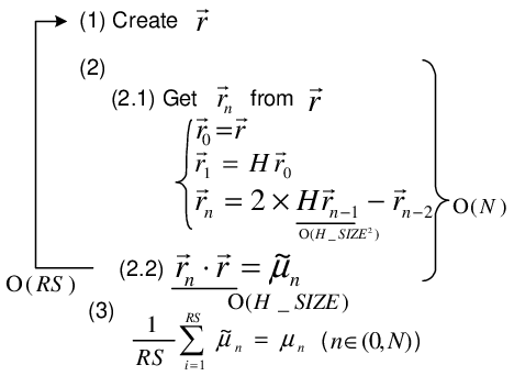
Figure 3 summarizes the KPM algorithm. The step (1) generates randomly a vector $\overrightarrow{r}$ that the number of elements is $H\_SIZE$ (this equals to the $D$ in section II-A). The step (2) gets $\overrightarrow{r}_{n}$ from $\overrightarrow{r}_{n-1}$ and $\overrightarrow{r}_{n-2}$ recursively calculating a matrix multiply of $H$ and $\overrightarrow{r}_{n-1}$ in the step (2.1). This multiplication is very hard to parallelize using MPI or OpenMP because of the dependencies due to the recursive iteration although the part needs the most intensive calculation. Then a dot product is calculated using $\overrightarrow{r}_{n}$ again with $\overrightarrow{r}$ at the step (2.2) and generates $\tilde{\mu}_{n}$ . Then the generation of the $\tilde{\mu}_{n}$ is iterated for $RS$ times. This means each generation of $\tilde{\mu}_{n}$ can be massively parallelized on GPUs. Finally, the average of all the $\tilde{\mu}_{n}$ s is generated at the step (3). N $\mu_{n}$ s are finally generated from the RS-time iterations of the step (1) and (2). This generation of the moments achieves the objective of the KPM. This summation to generate $\tilde{\mu}_{n}$ can be parallelized on GPU. Therefore, implemented on GPUs, two parallel processing parts are entirely performed during the evaluation of the moments using KPM: a) generation of $\tilde{\mu}_{n}$ and b) generation of $\mu_{n}$ . The maximum number of parallelism at the both a) and b) parts becomes the $SR$ because the total number of threads executed in the stream processors is $SR$ . Here, GPU has an architectural restriction to the number of threads in a thread block referred as BLOCK_SIZE in this paper. Therefore, the number of thread blocks becomes $RS/BLOCK\_SIZE$ . Considering the parallelization techniques above, let us explain the implementation of a kernel program on CUDA that invokes both the a) and b) parts.

III-B Implementation

We have implemented a kernel program for GPU using CUDA. The kernel receives the $H\_SIZE$ , $N$ that is the number of moments and $RS$ as the arguments. All calculations are performed based on double precision. The kernel includes two important concepts. One is how to keep high parallelism. Another is an effective memory management for the parallelism.

III-B1 Parallelization of calculations

As we discussed in the last section, two heavy calculation parts (the a) and the b)) should be parallelized and it would give the largest impact for the speedup.

Figure 4 a) shows the generation part for the $\overrightarrow{r}_{n}$ . $\overrightarrow{r}_{n}$ needs $\overrightarrow{r}_{n-1}$ , $\overrightarrow{r}_{n-2}$ and $\overrightarrow{r}$ that is randomly generated. These four vectors are obtained in the global memory and each block will write those vectors swapping the pointers. Here the number of blocks is $RS/BLOCK\_SIZE$ . In each block, $BLOCK\_SIZE$ stream processors are concurrently working to generate a part of those vectors including the random number generation for $\overrightarrow{r}$ . Therefore, this part will be fully parallelized into the total number of stream processors equipped on GPUs. This part will generate $\tilde{\mu}_{1}$ , $\tilde{\mu}_{2}$ … $\tilde{\mu}_{N}$ using $\overrightarrow{r}$ and $\overrightarrow{r}_{n}$ for $N$ time iteration.

Figure 4 b) depicts the parallelization of generation for $\mu_{n}$ . It performs just parallel summations for generating a scalar $\mu_{n}$ where all blocks works in parallel.

III-B2 Memory consumption

Let us consider the required memory amount for the operations in Figure 4 in the case of double precision. For the operation a), because four $\overrightarrow{r}$ vectors are stored in the global memory for a block. Each $\overrightarrow{r}$ vector has $H\_SIZE$ elements. Therefore, this part consumes $Number~of~Blocks\times 4\times H\_SIZE\times 8$ bytes. The operation b) is parallelized into the number of blocks. Each block performs a part of summation using N $\tilde{\mu}$ s. The length of $\tilde{\mu}$ s is $H\_SIZE$ . Therefore, it needs totally $Number~of~Blocks\times N\times H\_SIZE\times 8$ bytes.

The operation a) writes $\tilde{\mu}_{n}$ into the global memory. This needs to be kept with $\overrightarrow{r}$ vectors simultaneously. Therefore, the total number of memory is $Number~of~Blocks\times H\_SIZE\times(8\times N+32)$ .

Due to the recursive relationships among $\overrightarrow{r}_{n}$ , $\overrightarrow{r}_{n-1}$ and $\overrightarrow{r}_{n-2}$ , the KPM is treated generally as one of very hard parallelized algorithms. However, as we can see in this section, on the GPU, a massively parallel environment, the KPM is fully parallelized due to the stream-based computing concept. Thus, we can expect an effective speedup that will be proportional to the number of stream-processors.

IV Experimental performance analysis

This section shows performance evaluations of the KPM implemented on GPU. The performance based on GPU is compared with the one based on CPU. The experimental environment is a PC that consists of an Intel’s Core i7 930 processor at 2.80GHz with 12GB DDR3 memory, and the NVIDIA Tesla C2050 with 3GB Memory is connected to the PCI Express bus. The configuration of the cache in the GPU is set to 16KB and the shared memory size is 48KB. The OS of the PC is the Cent OS of the Linux Kernel 2.6.18. The driver version of the GPU is 3.0. All KPM calculations are performed with double precision floating point. The CPU version is compiled with GCC 4.4.1 with O3 option.

We perform three kinds of performance analysis: (1) evaluation using actual sets of parameters, (2) the one with increasing calculation size and (3) the one with increasing memory usage. The first evaluation hires sets of parameters used in actual simulations of the meaningful model applied to the condensed matter physics field. The second evaluation analyses the behavior of the performances when the parameter $N$ is increased. This means that more intensive calculation is loaded to the CPU and the GPU following the increase of $N$ . The last evaluation shows the performance impacts when the $H\_SIZE$ is increased. This case needs the square sized memory to store the $H$ matrix that is increased by the impact of $H\_SIZE^{2}$ .

IV-A Performance analysis using actual simulation parameters

In the field of the computational condensed matter physics, the KPM is applied to a simulation to evaluate the DoS in a three dimensional lattice model. Let us consider a lattice model made of cubes in $10\times 10\times 10$ where an electron is placed in each corner. This model needs a Hamiltonian matrix sized in $1000\times 1000$ due to the presentations of correlations among the electrons at each corner. The significant characteristics of the matrix include that 1) it is sparse and symmetric and 2) any row contains seven non-zero elements with the condition where all diagonal ones are zeros and the other non-zero ones are $-1$ s.

We evaluate the DoS in the case of the lattice that we assumed above using the fixed parameters of the KPM with $S=14$ and $R=128$ . Varying $N$ from 128 to 1024 in the steps of $2^{n}$ , Figure 5 shows the execution times and the speedup comparing the performances on the CPU with the ones on the GPU. The speedup keeps 3.5 times for all the cases. This means that the simulation can be accelerated by the GPU and the execution time becomes almost 40% faster than the one on CPU at most.

We shall pickup two DoS data combinations from the parameter sets of Figure 5 and plot it to a graph as depicted in Figure 6. The graph shows the DoS when $N=256$ and $N=512$ . When $N$ is the smaller number, the truncation reduces to the resolution of the DoS. However, the processing time is smaller than the case of a large $N$ . Therefore, although the case of $N=512$ shows higher resolution of the DoS, it takes longer calculation time.

IV-B Performance analysis with increased intensive calculations

Obtaining the fixed parameters of $H\_SIZE=128$ , $R=14$ and $S=128$ , we measure the performances with varying the $N$ from 128 to 2048. The graph of the performances is illustrated in Figure 7. The graph shows the execution times with bars and the speedups (i.e. the CPU time is divided by the corresponding GPU time) with a line. As increasing the $N$ , that is, as increasing the calculation amount, the speedup increases to almost 4 times. This means that the performance with the higher intensive calculations affected by the larger $N$ causes higher effective data parallelism on GPU when the calculation amount is increased without changing the size of the memory usage. Thus, our implementation on GPU clearly achieves higher performance than the CPU-based KPM as increasing the calculation amount.

IV-C Performance analysis with increased memory usage

This analysis fixes $N=128$ , $R=14$ and $S=128$ . We vary $H\_SIZE$ from 512 to 4096 with the step of $2^{n}$ . The performance presents effects caused by increasing the memory usage. The graph of the performance is depicted in Figure 8. When the amount of memory usage increases, the number of memory accesses increases. Therefore, the CPU version needs to read/write the memory as increased the size of $\tilde{H}$ matrix. On the other hand, because the GPU can cache a part of the matrix into very fast shared memory and accesses the memory in the stream-based manner. Thus, the execution time of the GPU version does not increase more than the complexity ( $O(H\_SIZE^{2})$ ). This causes almost four times faster performance than the CPU version.

As we discussed in three kinds of evaluations above, the performances on GPU achieve better performances than the ones on CPU due to the highly parallelism caused by the GPU-based implementation explained in this paper. The implementation achieves the advanced performance even if it is applied to the actual examples from the condensed matter physics or the cases with hard conditions virtually when the amounts of the computation and the memory usage are increased. Thus, we have confirmed that the KPM is a suitable algorithm that fits well to the GPU environment and the performance acceleration accomplishes amazingly the high performance.

V Conclusions

This paper has proposed an implementation of the KPM widely used in the physics and the chemistry field to simulate various quantum states. Our GPU version shows about 4 times faster than the CPU one. Therefore, using a GPU, productivity of the moments for a quantum state is accelerated to four times. Therefore, the GPU version is expected to be used for various grand challenge simulations to find a new quantum state that resolves unknown physical theories in the natural phenomenon.

For the future plans, we are considering to quest a method to find the best block size used in the GPU that defines the size of the stream processors’ block. Moreover, the parallelization of the KPM on a message passing and a shared memory paradigm is also challenging because the recursive reference to get $\overrightarrow{r}_{n}$ becomes a bottleneck to be parallelized in fine-grain. Moreover, we are also planning to extend the GPU-based implementation to a GPU cluster for its parallelization.

Acknowledgment

This work is partially supported by the Japan Science Technology Agency (JST) PRESTO program.

References

[1] J. G. Bednorz and K. A. Müller, “Possible high ${T}_{c}$ superconductivity in the Ba-La-Cu-O system,” Zeitschrift für Physik B Condensed Matter, vol. 64, no. 2, pp. 189–193, 1986.
[2] M. Yamashita, N. Nakata, Y. Senshu, M. Nagata, H. M. Yamamoto, R. Kato, T. Shibauchi, and Y. Matsuda, “Highly mobile gapless excitations in a two-dimensional candidate quantum spin liquid,” Science, vol. 328, no. 5983, pp. 1246–1248, June 2010.
[3] E. Dagotto, “Correlated electrons in high-temperature superconductors,” Review of Modern Physics, vol. 66, no. 3, pp. 763–840, July-September 1994.
[4] S. Yamada, T. Imamura, T. Kano, Y. Ohashi, H. Matsumoto, and M. Machida, “Ultra large-scale exact-diagonalization for confined fermion-hubbard model on the earth simulator: Exploration of superfluidity in confined strongly correlated systems,” Journal of the Earth Simulator, vol. 7, no. , pp. 23–35, June 2007.
[5] W. Foulkes, L. Mitas, R. Needs, and G. Rajagopal, “Quantum monte carlo simulations of solids,” Review of Modern Physics, vol. 73, no. 1, pp. 33–83, January 2001.
[6] S. White, “Density matrix formulation for quantum renormalization groups,” Physical Review Letters, vol. 69, no. 19, pp. 2863–2866, November 1992.
[7] ——, “Density-matrix algorithms for quantum renormalization groups,” Physical Review B, vol. 48, no. 14, pp. 10 345–1035, October 1993.
[8] U. Schollwöck, “The density-matrix renormalization group,” Review of Modern Physics, vol. 77, no. 1, pp. 259–315, January 2005.
[9] S. Yamada, M. Okumura, and M. Machida, “Direct extension of density-matrix renormalization group to two-dimensional quantum lattice systems: Studies of parallel algorithm, accuracy, and performance,” Journal of the Physical Society of Japan, vol. 78, no. 9, p. 094004, September 2009.
[10] A. Weiße, G. Wellein, A. Alvermann, and H. Fehske, “The kernel polynomial method,” Review of Modern Physics, vol. 78, no. 1, pp. 275–306, January 2006.
[11] J. D. Owens, D. Luebke, N. Govindaraju, M. Harris, J. Kruger, A. E. Lefohn, and T. J. Purcell, “A survey of general-purpose computation on graphics hardware,” in Eurographics 2005, State of the Art Reports, Aug. 2005, pp. 21–51.
[12] NVIDIA Corporation, “CUDA: Compute Unified Device Architecture programming guide, http://developer.nvidia.com/cuda.”

	$\displaystyle\|r_{0}\rangle$	$\displaystyle=\|r\rangle\,,\quad\|r_{1}\rangle=\tilde{H}\|r_{0}\rangle\,,$		(17)
	$\displaystyle\|r_{n+2}\rangle$	$\displaystyle=2\tilde{H}\|r_{n+1}\rangle-\|r_{n}\rangle\,.$		(18)

Performance Acceleration of Kernel Polynomial Method Applying Graphics Processing Units

Abstract

Index Terms:

I Introduction

II Background and definitions

II-A Kernel polynomial method

II-A1 Definition

II-A2 Application to quantum systems

II-A3 Stochastic evaluation of traces

II-A4 Numerical complexity

II-B General purpose computing on GPUs

II-B1 GPU architecture

II-B2 CUDA

III Kernel polynomial method applying GPUs

III-A Design for massively parallel platform

III-B Implementation

III-B1 Parallelization of calculations

III-B2 Memory consumption

IV Experimental performance analysis

IV-A Performance analysis using actual simulation parameters

IV-B Performance analysis with increased intensive calculations

IV-C Performance analysis with increased memory usage

V Conclusions

Acknowledgment

References

Performance Acceleration of Kernel Polynomial Method
Applying Graphics Processing Units