Strong-coupling effective action(s) for $SU(3)$ Yang-Mills Thanks: Presented at Excited QCD 2011 - February 20–25, Les Houches

Among the possible approaches to the study of Lattice QCD, effective theories play an important rôle, sometimes opening the way to subjects otherwise inaccessible, giving a deeper understanding of the physics at play, or even simply reducing the computational efforts involved. A desirable condition is that the effective theory is motivated by first principles and retains the original symmetries. The history of QCD effective theories is rather long; this work aims at providing the final results for the strong-coupling approach presented in [1].

The effective theories considered in this work re-express the partition function of a $(3+1)$-dimensional Yang-Mills $SU(N)$ lattice theory (all explicit calculations refer to $N=3$) as a three-dimensional model with complex numbers as per-site degrees of freedom, the (traced) Polyakov loops in the 4D system $L_{x}\equiv\mathrm{Tr}\prod_{\tau=1}^{N_{\tau}}U_{0}(x,\tau)$:

The effective models will exhibit various spin-like interaction terms $S_{n}$, each with a specific coupling $\lambda_{n}$ which is a function of the imaginary-time extent $N_{\tau}$ of the 4D lattice and its (bare) coupling $\beta$. The strong-coupling series for the $\lambda_{n}(\beta,N_{\tau})$ employs a character expansion and then the moment-cumulant formalism [1, 2]; here we only report the final formulae.

Of the (infinitely many) interaction terms, we consider the three featuring the lowest order in $\beta$ (or in $u\equiv a_{f}(\beta)\simeq\beta/18+\mathcal{O}(\beta^{2})$, see e. g. [2]): nearest- and next-to-nearest-neighbour fundamental representation ($\lambda_{1}S_{1}$, $\lambda_{2}S_{2}$), and nearest-neighbour adjoint interaction ($\lambda_{a}S_{a}$). We study three different effective theories: one with only the $\lambda_{1}$ interaction, one with $(\lambda_{1},\lambda_{2})$, and the last with the $(\lambda_{1},\lambda_{a})$ terms. We parametrise $L$ as:¹¹ 1 We note that the measure used in [1] contains an error corrected here.

The effective theories studied numerically are given by:²² 2 $<\hskip-3.50006pti,j\hskip-3.50006pt>$ denotes nearest-neighbours and $[k,l]$ next-to-nearest-neighbours. $Z_{(1)}\equiv Z_{(1,2)}|_{\lambda_{2}=0}$,

In [1] we presented the mappings $\lambda_{n}\leftrightarrow\beta$ for even $N_{\tau}$; here we provide in addition $N_{\tau}=1,3$: $\lambda_{1}(u;1)=u$, $\lambda_{2}(u;1)=0$ and $\lambda_{a}(u;1)=v$; for $N_{\tau}=3$ the $\lambda_{a}$ map follows the general formula, while:

All three models were simulated on cubic systems with $N_{s}^{3}$ sites and periodic boundary conditions via a Metropolis accept/reject procedure. Looking at the expressions in Eq. 4, one realises that at sufficiently high couplings a “sign problem” might occur for negative values of $\mathrm{Re}(L_{i}L^{*}_{j})$: to take care of this, the simulations uses weights $|(1+2\lambda_{1}\mathrm{Re}L_{i}L^{*}_{j})|$ (and similarly for the other terms) and folds the sign into the observable, which is subsequently reweighted to get the correct answer. It turns out that, within the range of couplings of interest, this problem is very mild and the average sign of a configuration never drops below 0.999.

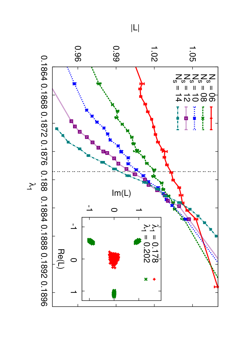
One-coupling model. A first inspection of the distribution of $L_{x}$ at different couplings confirms the existence of a phase transition at some finite $\lambda_{1,c}^{(1)}$ (fig. 1). More quantitatively, we use as basic observable

We measure the Binder cumulant and the susceptibility:

the minimum of the former and the maximum of the latter (see fig. 1) are used as size-dependent criticality estimators $\lambda_{B,\chi}(N_{s})$, and a finite-size scaling fit is then attempted on both, with first-order scaling law

Data from systems of side $N_{s}=6,8,10,12,14$ allowed for two independent and consistent estimates of the infinite-volume critical point, averaged to $\lambda_{1,c}^{(1)}=0.187885(30)$. Further evidence in support of the first-order nature of the transition comes from the scaling of the $y$-coordinates of the extrema of the observables in Eq. 7: we found for both (fig. 2)

with $y_{\chi}^{\infty}>0$ and $y_{B}^{\infty}=0.66277(7)$: the latter, as required, is lower than $2/3$, and consistent with the estimate $y_{B,\infty}^{*}=0.6617(15)$ coming from locating the two maxima $|L|_{1,2}$ in the distribution of $|L|$ at criticality [3].

Two-coupling model $(\lambda_{1},\lambda_{2})$. In the two-parameter cases, the $\beta_{c}$ of the original gauge theory is found by intersecting the critical line of the models per se and one-dimensional manifolds encoding the original theory at $N_{\tau}$. Ten values of $\lambda_{2}\leq 0.01$ were fixed and the approach of the previous case was applied to all of them: a polynomial fit to $\lambda_{1}=a_{0}+a_{1}\lambda_{2}+a_{2}\lambda_{2}^{2}$ gives the curve in fig. 3, compatible with the value for $\lambda_{2}=0$, with $a_{i}=\{0.18787(2),-3.375(8),12.8(7)\}$.

Two-coupling model $(\lambda_{1},\lambda_{a})$. The same procedure led to a parametrisation of the critical line in the $(\lambda_{1},\lambda_{a})$ plane, with 13 sampled values of $\lambda_{a}\leq 0.12$. In this case the fitted function was $\lambda_{1}=c_{0}+c_{1}\lambda_{a}+c_{2}\lambda_{a}^{2}+c_{3}\lambda_{a}^{3}$ (fig. 3), with coefficients $c_{i}=\{0.18783(8),-0.50(2),-6.9(7),30.4(5.7)\}$.

The 4D data were taken from [4, 5], except the $N_{\tau}=1$ critical point which was determined with a dedicated set of standard $SU(3)$ Wilson action simulations. The values for $\beta_{c}(N_{\tau})$ are summarised in Table 1 and plotted in fig. 4, along with a plot of the ratio between the effective-theory result and the full 4D Yang-Mills outcome.

The discrepancy never exceeds $\sim 7$–$8$%; it is noteworthy that the one-coupling action seems to provide the best estimates at $N_{\tau}=1,2$. At low $N_{\tau}$, where $\beta$ is smaller, we expect the series expansion to show a better convergence; on the other hand, the particular shape of the mappings $\lambda_{i}(\beta)$ is such that, as $N_{\tau}$ increases, only the $\lambda_{1}$ coupling is important, which is the reason why the various results tend to converge one onto another.

It must be stressed that the present results, able to reproduce the critical points with some accuracy, are obtained with a rather small computational effort (3D instead of 4D and complex numbers instead of matrices), measurable in the range of a few days with an ordinary desktop PC. This is in contrast with the “inverse Monte Carlo” approach [6], which requires simulating the full theory in order to fix the coefficients; on the other hand, the latter technique is able to reproduce the theory on both sides of the transition.

An extension of the present work is currently being carried on, with the introduction of massive fermions in the effective formulation via a hopping-parameter expansion.

References

- [1] J. Langelage, S. Lottini, O. Philipsen, JHEP02 (2011) 057, [arXiv:arXiv:1010.0951v2 [hep-lat]].
- [2] I. Montvay, G. Münster, Quantum fields on a lattice, Cambridge, UK: Univ. Pr. (1994) 491 p. (Cambridge monographs on mathematical physics).
- [3] J. Lee, J. M. Kosterlitz, Phys. Rev. B43 (1991) 3265.
- [4] J. Kogut, M. Stone, H. W. Wyld, Phys. Rev. Lett. 50 (1983) 393.
- [5] J. Fingberg, U. M. Heller, F. Karsch, Nucl. Phys. B 392 (1993) 493.
- [6] C. Wozar, T. Kaestner, A. Wipf, T. Heinzl, Phys. Rev. D 76 (2007) 085004 [arXiv:0704.2570 [hep-lat]].