First hyperfine resolved far-infrared OH spectrum from a star-forming regionThanks: Herschel is an ESA space observatory with science instruments provided by European-led Principal Investigator consortia and with important participation from NASA.

S. F. Wampfler Affiliation: Institute for Astronomy, ETH Zurich, 8093 Zurich, Switzerland S. Bruderer Affiliation: Max Planck Institut für Extraterrestrische Physik, Giessenbachstrasse 1, 85748 Garching, Germany L. E. Kristensen Affiliation: Leiden Observatory, Leiden University, PO Box 9513, 2300 RA Leiden, The Netherlands L. Chavarría Affiliation: Université de Bordeaux, Observatoire Aquitain des Sciences de l’Univers, F-33271 Floirac Cedex, France Affiliation: CNRS, UMR 5804, Laboratoire d’Astrophysique de Bordeaux, 2 rue de l’Observatoire, BP 89, F-33271 Floirac Cedex, France E. A. Bergin Affiliation: Department of Astronomy, The University of Michigan, 500 Church Street, Ann Arbor, MI 48109-1042, USA A. O. Benz Affiliation: Institute for Astronomy, ETH Zurich, 8093 Zurich, Switzerland E. F. van Dishoeck Affiliation: Max Planck Institut für Extraterrestrische Physik, Giessenbachstrasse 1, 85748 Garching, Germany Affiliation: Leiden Observatory, Leiden University, PO Box 9513, 2300 RA Leiden, The Netherlands G. J. Herczeg Affiliation: Max Planck Institut für Extraterrestrische Physik, Giessenbachstrasse 1, 85748 Garching, Germany F. F. S. van der Tak Affiliation: SRON Netherlands Institute for Space Research, PO Box 800, 9700 AV, Groningen, The Netherlands Affiliation: Kapteyn Astronomical Institute, University of Groningen, PO Box 800, 9700 AV, Groningen, The Netherlands J. R. Goicoechea Affiliation: Departamento de Astrofísica, Centro de Astrobiología (CSIC-INTA), 28850, Madrid, Spain S. D. Doty Affiliation: Department of Physics and Astronomy, Denison University, Granville, OH, 43023, USA F. Herpin Affiliation: Université de Bordeaux, Observatoire Aquitain des Sciences de l’Univers, F-33271 Floirac Cedex, France Affiliation: CNRS, UMR 5804, Laboratoire d’Astrophysique de Bordeaux, 2 rue de l’Observatoire, BP 89, F-33271 Floirac Cedex, France

accepted May 25, 2011

Abstract

OH is an important molecule in the H₂O chemistry and the cooling budget of star-forming regions. The goal of the Herschel key program ‘Water in Star-forming regions with Herschel’ (WISH) is to study H₂O and related species during protostellar evolution. Our aim in this letter is to assess the origin of the OH emission from star-forming regions and constrain the properties of the emitting gas. High-resolution observations of the OH ${}^{2}\Pi_{1/2}\penalty\ J=3/2-1/2$ triplet at $1837.8\penalty\ \mathrm{GHz}$ ( $163.1\penalty\ \mu$ m) towards the high-mass star-forming region W3 IRS 5 with the Heterodyne Instrument for the Far-Infrared (HIFI) on Herschel reveal the first hyperfine velocity-resolved OH far-infrared spectrum of a star-forming region. The line profile of the OH emission shows two components: a narrow component (FWHM $\approx 4-5\penalty\ \mathrm{km}\penalty\ \mathrm{s}^{-1}$ ) with partially resolved hyperfine structure resides on top of a broad (FWHM $\approx 30\penalty\ \mathrm{km}\penalty\ \mathrm{s}^{-1}$ ) component. The narrow emission agrees well with results from radiative transfer calculations of a spherical envelope model for W3 IRS 5 with a constant OH abundance of $x_{\mathrm{OH}}\approx 8\times 10^{-9}$ . Comparison with H₂O yields OH/H₂O abundance ratios of around $10^{-3}$ for $T\gtrsim 100\penalty\ \mathrm{K}$ and around unity for $T\lesssim 100\penalty\ \mathrm{K}$ , consistent with the current picture of the dense cloud chemistry with freeze-out and photodesorption. The broad component is attributed to outflow emission. An abundance ratio of OH/H₂O $\gtrsim 0.028$ in the outflow is derived from comparison with results of water line modeling. This ratio can be explained by a fast J-type shock or a slower UV-irradiated C-type shock.

Key Words.

Astrochemistry — Stars: formation — ISM: molecules — ISM: jets and outflows — ISM: individual objects: W3 IRS 5

1 Introduction

Newly-formed stars inject large amounts of energy into the ambient interstellar material through shocks and radiation, heating the surrounding gas and dust. In these warm regions, H₂O becomes one of the most abundant gas-phase molecules because water ice evaporates from the grain mantles and gas-phase formation routes become available. The hydroxyl radical (OH) is closely linked to both the H₂O formation and destruction through OH + H₂ $\Leftrightarrow$ H₂O + H as well as a byproduct of the H₂O photodissociation process in the presence of UV photons. A significant fraction of the gas cooling occurs through line emission in the far-infrared, including lines of $[$ O i $]$ , $[$ C ii $]$ , CO, H₂O, and OH (Giannini et al., 2001; van Kempen et al., 2010).

Observations of the OH far-infrared transitions first became possible with the Kuiper Airborne Observatory (e.g. Storey et al., 1981; Betz & Boreiko, 1989; Melnick et al., 1990, and references therein). OH was frequently detected in star-forming regions with ISO (Giannini et al., 2001; Goicoechea et al., 2006, e.g.) and with PACS (Wampfler et al., 2010) on board the Herschel Space Observatory (Pilbratt et al., 2010). Previously, OH was mainly observed through maser lines at cm wavelengths (Gaume & Mutel, 1987, for models see e.g. Cesaroni & Walmsley 1991). Observations carried out with ISO and PACS lack the spectral resolution needed to distinguish between OH emission from the quiescent envelope and the outflow, since no information on the line shape is obtained. Furthermore, the hyperfine structure of the OH lines remaines unresolved. The Heterodyne Instrument for the Far-Infrared (de Graauw et al., 2010, HIFI, ) on Herschel offers an adequate spectral resolution to resolve the 1837.8 GHz triplet of OH. Thus, optical depths and line widths to constrain the temperature and density of the emitting gas can be derived. A blended OH triplet was previously detected with HIFI from Orion KL (Crockett et al., 2010).

This letter presents the first hyperfine velocity resolved observations of OH obtained using HIFI from the well-studied high-mass star-forming region W3 IRS 5 located at a distance of 2 kpc (Hachisuka et al., 2006) with a total luminosity of $\sim 10^{5}\penalty\ \mathrm{L}_{\sun}$ (Helmich & van Dishoeck, 1997; Boonman et al., 2003; van der Tak et al., 2005; Chavarría et al., 2010; Benz et al., 2010, e.g. ).

2 Observations and data reduction

The OH triplet at 1837.747, 1837.817 and 1837.837 GHz from W3 IRS 5 ( $\alpha_{2000}=02^{\mathrm{h}}25^{\mathrm{m}}40\aas@@fstack{s}60$ , $\delta_{2000}=+62\degr 05\arcmin 51\aas@@fstack{\prime\prime}0$ ) was observed with HIFI on Herschel. The observations were carried out as part of the ‘Water in Star-Forming Regions with Herschel’ (WISH) key program (van Dishoeck et al., 2011). W3 IRS 5 was observed on July 29^th 2010 (obsid 1342201666) in dual beam switch mode with an on-source integration time of 17 min. The beam size (HPBW) at 1837 GHz is about $12\arcsec$ . The average system temperature was 1245 K. The wide band spectrometer (WBS) offers a nominal resolution of 1.1 MHz, corresponding to a velocity resolution of about $0.18\penalty\ \mathrm{km}\penalty\ \mathrm{s}^{-1}$ at 1837 GHz. The OH triplet at 1834.7 GHz was not observed.

HIFI data were reduced using the Herschel interactive processing environment (Ott, 2010, HIPE v4.0.0, ) and the GILDAS-CLASS¹¹ 1 http://www.iram.fr/IRAMFR/GILDAS software. The H and V polarizations were combined, reaching $T_{\mathrm{rms}}\approx 0.1\penalty\ \mathrm{K}$ . We subtracted a first order polynomial from the spectra and calibrated to $T_{\mathrm{mb}}$ scale using a main beam efficiency of 0.70. Molecular data (Table 1) are taken from the Leiden atomic and molecular database LAMDA²² 2 http://www.strw.leidenuniv.nl/ $\sim$ moldata/ (Schöier et al., 2005) with data from the JPL catalog³³ 3 http://spec.jpl.nasa.gov (Pickett et al., 1998) and collisional rate coefficients by Offer et al. (1994).

The calibration uncertainty of band 7b is currently estimated to $\lesssim 32\%$ and is mainly caused by the unknown side band gain ratio. The uncertainty reduces to about 10% for a ratio close to unity. The errors on the integrated intensities are only fitting errors and do not include the calibration uncertainty. The velocity calibration is uncertain by $\sim 0.2\penalty\ \mathrm{km}\penalty\ \mathrm{s}^{-1}$ and could partially explain the $\sim 0.5\penalty\ \mathrm{km}\penalty\ \mathrm{s}^{-1}$ offsets of the line peaks from the source velocity of $\varv_{\mathrm{lsr}}=-38.4\penalty\ \mathrm{km}\penalty\ \mathrm{s}^{-1}$ (van der Tak et al., 2000).

3 Results

HIFI clearly detects the OH triplet at around 1837.8 GHz ( $163.1\penalty\ \mu$ m) towards W3 IRS 5 (Fig. 1). For the first time, the hyperfine components of the line triplet are spectrally resolved.

Two components dominate the line shape: the line profile shows narrow components residing on top of a broad emission feature, similar to that found by Chavarría et al. (2010) for H₂O lines in W3 IRS 5 and Kristensen et al. (2010) in low-mass YSOs. The narrow components with full widths at half maximum (FWHM) of $\sim 4-5\penalty\ \mathrm{km}\penalty\ \mathrm{s}^{-1}$ are centered close to the positions expected from the hyperfine pattern. The lines are split by $20.2\penalty\ \mathrm{MHz}$ ( $3.3\penalty\ \mathrm{km}\penalty\ \mathrm{s}^{-1}$ ) towards the blue and $70.2\penalty\ \mathrm{MHz}$ ( $11.5\penalty\ \mathrm{km}\penalty\ \mathrm{s}^{-1}$ ) towards the red relative to the middle line. Therefore, the ( $F=2+\rightarrow 1-$ ; Tab. 1) and ( $F=1+\rightarrow 0-$ ) transitions are blended, while the ( $F=1+\rightarrow 1-$ ) transition is resolved. The underlying broad component with a FWHM of $\sim 30\penalty\ \mathrm{km}\penalty\ \mathrm{s}^{-1}$ consists of the three blended hyperfine components, each with $\Delta{\rm\varv}\sim 20$ km s^-1. The hyperfine pattern is unresolved in the broad component.

Gaussian fits to the narrow components are presented in the online appendix (Sec. A). The derived hyperfine intensity ratios (1: $3\pm 0.5$ : $1.5\pm 0.3$ ) deviate from the prediction of LTE in the optically thin limit ( $\sim A_{\mathrm{ul}}g_{\mathrm{u}}$ , 1:5:2). Pumping by far-infrared dust continuum radiation, line overlap, and optical depth may all contribute to the observed hyperfine anomaly. Modeling results (Sec. 3.1) indicate that at least the $2+\rightarrow 1-$ line is optically thick. Based on comparison with spherical envelope models (Sec. 3.2), we attribute the narrow components to OH emission from the hot parts of the envelope.

The broad component in OH is most likely associated with outflow emission. Its integrated intensity is around $37\penalty\ \mathrm{K}\penalty\ \mathrm{km}\penalty\ \mathrm{s}^{-1}$ (Sec. A). A similar component can also be identified in the line profiles of other species like CO and H₂O (Sec. B) from recent Herschel results and ground-based observations (Hasegawa et al., 1994; Boonman et al., 2003; Chavarría et al., 2010, e.g. ).

Table 1: Molecular data of the observed OH transitions between the

{}^{2}\Pi_{1/2}

3/2 and 1/2 excited states.

Transition	Frequency	$A_{\mathrm{ul}}$	$g_{u}$	$g_{l}$	Shift
F, P	[GHz]	[s^-1]			[km s^-1]
$1+\rightarrow 1-$	1837.7466	2.1(-2)	3	3	11.5
$2+\rightarrow 1-$	1837.8168	6.4(-2)	5	3	0.0
$1+\rightarrow 0-$	1837.8370	4.3(-2)	3	1	-3.3

$A(B)\equiv A\times 10^{B}$ . The last column denotes the velocity shift relative to the component with the largest Einstein A coefficient.

Refer to caption — Figure 1: HIFI spectrum of the OH triplet at 1837.8 GHz with half the dual-sideband continuum. The expected positions of the lines and the source velocity are labeled. The blue lines show the best fit from the slab models and the outflow component separately.

3.1 Slab Models

As a first modeling step to derive OH column densities, the slab method outlined in Bruderer et al. (2010, appendix B) is used. This method calculates the molecular spectrum from two slabs – one representing the envelope and one the outflow – in front of a continuum source, determined from the observed continuum flux. The slabs are assumed to cover the entire continuum source. The free parameters describing each slab are the OH column density $N_{\mathrm{OH}}$ , the excitation temperature $T_{\mathrm{ex}}$ (assumed to be equal for all hyperfine transitions), the line width $\Delta{\mathrm{\varv}}$ , and the position of the line center ${\mathrm{\varv}}_{\mathrm{lsr}}$ . Overlap between different hyperfine components of OH is taken into account. To constrain the free parameters ( $N_{\rm OH}$ , $T_{\rm ex}$ , $\Delta{\rm\varv}$ and ${\rm\varv}_{\rm lsr}$ ), the $\chi^{2}$ between observation and model is minimized using an uncertainty of $T_{\mathrm{rms}}\sim 0.1\penalty\ \mathrm{K}$ .

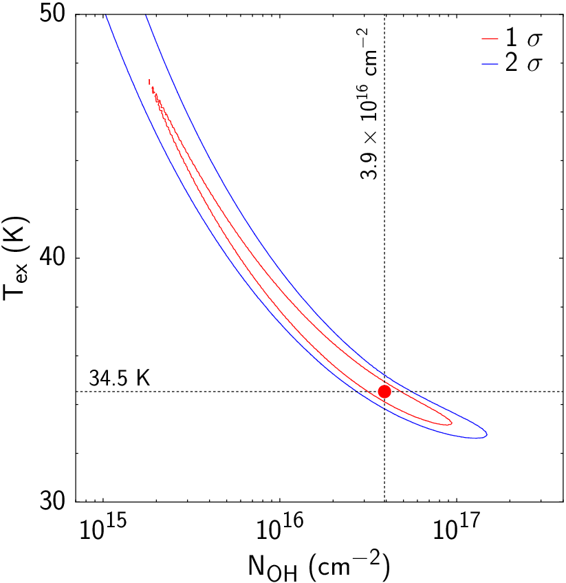
The resolved hyperfine triplet structure of the narrow (envelope) component allows us to constrain the column density and the excitation temperature of the emitting gas simultaneously. Results of the best fitting slab models for the narrow component with a reduced $\chi^{2}=1.2$ are presented in Table 2. A peak line opacity of $\tau=1.8$ is reached ( $2+\rightarrow 1-$ transition) and the $1+\rightarrow 0-$ and $1+\rightarrow 1-$ peaks have optical depths of $\tau=0.8$ and $\tau=0.4$ , respectively. Figure 4 of the online appendix shows the $1\sigma$ and $2\sigma$ contours for the column density and excitation temperature. The OH column densities within the $1\sigma$ interval range from $N_{\rm OH}=2\times 10^{15}-1\times 10^{17}$ cm^-2, depending on $T_{\mathrm{ex}}$ , and thus vary by almost two orders of magnitude.

A broad (outflow) component can be clearly identified in the spectrum, but its hyperfine components are not resolved. Thus, it is not possible to determine an excitation temperature of the broad emission from the spectrum. Assuming $T_{\rm ex}=100$ K, a column density of $N_{\rm OH}=2.0\times 10^{14}$ cm^-2 is obtained by fitting the line wings only. A lower limit on the OH column density of $N_{\rm OH}\geq 7.2\times 10^{13}$ cm^-2 is derived by assuming that the excitation temperature is equal to the upper level energy (270 K) of the transition. Both fits yield a line width of $\Delta\varv=21.9$ km s^-1 and a line position $\varv_{\rm lsr}=-35.7\penalty\ \mathrm{km}\penalty\ \mathrm{s}^{-1}$ . The line optical depth is $\tau<0.01$ for these excitation temperatures. An optical depth of $\tau=1$ is reached for $T_{\rm ex}<34$ K and no good fit can be obtained for $T_{\rm ex}\lesssim 32$ K. In the following, $T_{\rm ex}=270\penalty\ \mathrm{K}$ is assumed.

Table 2: Beam-averaged column density

N_{\rm OH}

, excitation temperature

T_{\rm ex}

, line width

\Delta\varv

, and line position

\varv_{\rm lsr}

of the best fit slab model.

	$N_{\rm OH}$	$T_{\rm ex}$	$\Delta\varv$	$\varv_{\rm lsr}$	fit range
	[cm^-2]	[K]	[km/s]	[km/s]	[km/s]
O	$\geq$ 7.2(13)	270.0^a	21.9	-35.7	[-60,-47.5], [-22,-10]
E	3.9(16)	34.5	3.3	-37.7	[-43,-35], [-30,-23]

^a fixed (see text). $A(B)\equiv A\times 10^{B}$ . O = outflow, E = envelope.

To convert the column density into an OH abundance in the outflow, the ¹²CO(3-2) observation of Hasegawa et al. (1994) was used to derive $N_{\mathrm{H}_{2}}=1.3\times 10^{21}\penalty\ \mathrm{cm}^{-2}$ with RADEX (van der Tak et al., 2007), assuming a CO/H₂ abundance ratio of $10^{-4}$ , a density of $10^{5}\penalty\ \mathrm{cm}^{-3}$ , and a temperature of $60\penalty\ \mathrm{K}$ , as derived in their paper. This H₂ column density converts the lower limit of $N_{\rm OH}\geq 7.2\times 10^{13}$ cm^-2 into a lower limit on the OH abundance of $x_{\mathrm{OH}}=N_{\mathrm{OH}}/N_{\mathrm{H}_{2}}\geq 5.5\times 10^{-8}$ .

3.2 Spherical model of the envelope

In addition to the slab modeling, the narrow emission component is compared to the results from full radiative transfer models using the ‘RATRAN’ code (Hogerheijde & van der Tak, 2000). The physical structure of W3 IRS 5 is taken from van der Tak et al. (2000) with a power-law density profile ranging from $n=10^{5}-10^{8}\penalty\ \mathrm{cm}^{-3}$ and temperatures $50\lesssim T\lesssim 950\penalty\ \mathrm{K}$ within the Herschel beam at $1837\penalty\ \mathrm{GHz}$ . Dust and gas temperatures are assumed to be equal. Far-infrared excitation by the dust continuum for $T_{\mathrm{dust}}$ is included. We also adopt their distance (2.2 kpc) for consistency. Dust opacities based on grains with thin ice mantles are assumed (Ossenkopf & Henning, 1994, table 1, column 5). The molecular abundance is assumed to be constant throughout the envelope, because this is the simplest structure yielding a good fit to the line profiles. Figure 2 shows the comparison between model and data, where the best fitting slab model for the broad component (cf. Sec. 3.1) is subtracted from the observation, leaving only the narrow component for a simpler comparison.

Models assuming an OH abundance of $x_{\mathrm{OH}}=(0.5-1)\times 10^{-8}$ agree reasonably well with the observed narrow components. RATRAN does not treat line overlap and overlap effects can therefore not be treated accurately for optically thick lines. Thus, we have simply added the intensities of the components as would be appropriate in the optically thin limit.

The spherical envelope models are also consistent with the $79,84$ and $119\penalty\ \mu\mathrm{m}$ lines being in absorption, as observed in the unpublished spectral scan obtained with PACS on Herschel. The $79$ and $119\penalty\ \mu\mathrm{m}$ transitions are connected to the ground ${}^{2}\Pi_{3/2}$ level and therefore prone to absorption. A quantitative analysis is not possible because the central spatial pixel of the detector is saturated.

4 Discussion

Insight into the water chemistry can be gained by comparing OH and H₂O abundances, because these species are linked through the OH + H₂ $\Leftrightarrow$ H₂O + H reactions. Chavarría et al. (2010) identify broad and narrow components in H₂O line profiles from W3 IRS 5 similar to OH. OH/H₂O abundance ratios can be derived separately for gas of the envelope and the outflow.

From the spherical non-LTE envelope models, which do not consider overlap of hyperfine components, we find an OH abundance of $x_{\mathrm{OH}}\approx 8\times 10^{-9}$ for W3 IRS 5. New calculations of the H₂O abundance $x_{\mathrm{H}_{2}\mathrm{O}}$ in the envelope, based on the work by Chavarría et al. (2010) but recalculated using the same physical structure as for OH, yield $x_{\mathrm{H}_{2}\mathrm{O}}=10^{-5}$ for $T\geq 100\penalty\ \mathrm{K}$ and $x_{\mathrm{H}_{2}\mathrm{O}}=10^{-8}$ for $T<100\penalty\ \mathrm{K}$ . This allows us to estimate the OH/H₂O abundance ratios: H₂O is about three orders of magnitude more abundant in the inner envelope ( $T\geq 100\penalty\ \mathrm{K}$ ), while the OH/H₂O ratio is around unity in the outer part ( $T<100\penalty\ \mathrm{K}$ ). The same conclusion is reached in the best fit H₂O abundance structure of Boonman et al. (2003) to ISO and SWAS data, which was derived with the same physical model as adopted here.

The inferred OH/H₂O ratios in the envelope are consistent with the current picture of the water chemistry in dense clouds (Hollenbach et al., 2009; van Dishoeck et al., 2011, for detailed discussion of processes see). Different paths can increase the gas-phase H₂O abundance in the inner part of protostellar envelopes. At $T\geq 100\penalty\ \mathrm{K}$ , H₂O starts to evaporate from the ice mantles of dust grains. When temperatures of $T\gtrsim 230\penalty\ \mathrm{K}$ are reached, which are typical for the innermost parts of high-mass protostellar envelopes, H₂O can be rapidly formed in the gas phase through OH + H₂ $\Rightarrow$ H₂O + H. In this case, OH is only a transient step of the H₂O formation process and thus OH/H₂O $\ll 1$ in the absence of UV photons. In the outer envelope, low-temperature gas-phase chemistry provides $x_{\mathrm{OH}}\approx 10^{-8}$ (Doty et al., 2002, Fig. 11). At the outer edge, H₂O and OH can be released into the gas phase by photodesorption from grain mantles. Öberg et al. (2009) and Andersson & van Dishoeck (2008) find from laboratory data and theoretical calculations that roughly equal amounts of OH and H₂O are released at low temperatures. Depending on the optical depth of the lines, this outer layer may dominate the emission.

The slab model method outlined in Sec. 3.1 is also used to estimate the H₂O abundance in the outflow component. Availability of HIFI para-H₂O $2_{0,2}-1_{1,1}$ (Chavarría et al., 2010, from ) and unpublished $2_{1,1}-2_{0,2}$ (Chavarria et al. in prep.) and $3_{3,1}-4_{0,4}$ data allow us to constrain $N_{\mathrm{p-H}_{2}\mathrm{O}}$ and the para-H₂O excitation temperature in the outflow simultaneously. We find $N_{\mathrm{p-H}_{2}\mathrm{O}}=6.4\times 10^{14}$ cm^-2 and thus $N_{\mathrm{H}_{2}\mathrm{O}}=2.6\times 10^{15}$ cm^-2 for an assumed ortho- to para-H₂O ratio of 3:1. The water abundance is calculated to be $2.1\times 10^{-6}$ with $N_{\mathrm{H}_{2}}=1.25\times 10^{21}\penalty\ \mathrm{cm}^{-2}$ . Under the assumption that the OH and H₂O emission arise from the same gas, we can calculate a lower limit of 0.028 on the OH/H₂O abundance ratio in the outflow of W3 IRS 5. This limit is consistent with the emission originating in either a fast ( $\varv>60\penalty\ \mathrm{km}\penalty\ \mathrm{s}^{-1}$ ), dissociative J-type shock (Neufeld & Dalgarno, 1989) or a slower UV-irradiated C-type shock (Wardle, 1999, $\varv\sim$ 20–30 km s^-1,). Standard C-type shocks underproduce the observed column density ratio by one order of magnitude or more (Kristensen et al. in prep.). It is not possible to distinguish between the two types of shocks with the current data and availability of model results.

5 Conclusions

The OH lines at $1837.8\penalty\ \mathrm{GHz}$ from W3 IRS 5 detected with HIFI consist of two components: a broad component, where the triplet components are blended because of the large individual line widths, and a narrow component with velocity resolved hyperfine structure on top. These results indicate that OH emission observed at a lower spectral resolution, e.g. with PACS, can be a blend of envelope and outflow contributions. Low-mass sources reach lower temperatures than the high-mass counterparts at the projected distance of the Herschel beam. From RATRAN models of low-mass sources we thus find a lower excitation, resulting in a weaker envelope contribution to the OH $1837\penalty\ \mathrm{GHz}$ lines than from W3 IRS 5, consistent with the results for HH 46 in Wampfler et al. (2010). Because the broad component also appears in the line profiles of other species from W3 IRS 5, in particular those of CO and H₂O, the outflow is the most likely origin of the emission. Comparison with H₂O yields a lower limit on the OH/H₂O abundance ratio of 0.028, consistent with an origin from a fast J-type shock or a slower UV-irradiated C-type shock. The narrow emission agrees well with spherical envelope models with a constant OH abundance of $x_{\mathrm{OH}}\approx 8\times 10^{-9}$ . Comparison with new H₂O results based on Chavarría et al. (2010) give OH/H₂O $\approx 1$ for $T<100\penalty\ \mathrm{K}$ and OH/H₂O $\approx 10^{-3}$ at $T\gtrsim 100\penalty\ \mathrm{K}$ , consistent with the current picture of the dense cloud chemistry with freeze-out.

References

Andersson & van Dishoeck (2008) Andersson, S. & van Dishoeck, E. F. 2008, A&A, 491, 907
Benz et al. (2010) Benz, A. O., Bruderer, S., van Dishoeck, E. F., et al. 2010, A&A, 521, L35+
Betz & Boreiko (1989) Betz, A. L. & Boreiko, R. T. 1989, ApJ, 346, L101
Boonman et al. (2003) Boonman, A. M. S., Doty, S. D., van Dishoeck, E. F., et al. 2003, A&A, 406, 937
Bruderer et al. (2010) Bruderer, S., Benz, A. O., van Dishoeck, E. F., et al. 2010, A&A, 521, L44+
Cesaroni & Walmsley (1991) Cesaroni, R. & Walmsley, C. M. 1991, A&A, 241, 537
Chavarría et al. (2010) Chavarría, L., Herpin, F., Jacq, T., et al. 2010, A&A, 521, L37+
Crockett et al. (2010) Crockett, N. R., Bergin, E. A., Wang, S., et al. 2010, A&A, 521, L21+
de Graauw et al. (2010) de Graauw, T., Helmich, F. P., Phillips, T. G., et al. 2010, A&A, 518, L6+
Doty et al. (2002) Doty, S. D., van Dishoeck, E. F., van der Tak, F. F. S., & Boonman, A. M. S. 2002, A&A, 389, 446
Gaume & Mutel (1987) Gaume, R. A. & Mutel, R. L. 1987, ApJS, 65, 193
Giannini et al. (2001) Giannini, T., Nisini, B., & Lorenzetti, D. 2001, ApJ, 555, 40
Goicoechea et al. (2006) Goicoechea, J. R., Cernicharo, J., Lerate, M. R., et al. 2006, ApJ, 641, L49
Hachisuka et al. (2006) Hachisuka, K., Brunthaler, A., Menten, K. M., et al. 2006, ApJ, 645, 337
Hasegawa et al. (1994) Hasegawa, T. I., Mitchell, G. F., Matthews, H. E., & Tacconi, L. 1994, ApJ, 426, 215
Helmich & van Dishoeck (1997) Helmich, F. P. & van Dishoeck, E. F. 1997, A&AS, 124, 205
Hogerheijde & van der Tak (2000) Hogerheijde, M. R. & van der Tak, F. F. S. 2000, A&A, 362, 697
Hollenbach et al. (2009) Hollenbach, D., Kaufman, M. J., Bergin, E. A., & Melnick, G. J. 2009, ApJ, 690, 1497
Kristensen et al. (2010) Kristensen, L. E., Visser, R., van Dishoeck, E. F., et al. 2010, A&A, 521, L30+
Melnick et al. (1990) Melnick, G. J., Stacey, G. J., Lugten, J. B., Genzel, R., & Poglitsch, A. 1990, ApJ, 348, 161
Neufeld & Dalgarno (1989) Neufeld, D. A. & Dalgarno, A. 1989, ApJ, 340, 869
Öberg et al. (2009) Öberg, K. I., Linnartz, H., Visser, R., & van Dishoeck, E. F. 2009, ApJ, 693, 1209
Offer et al. (1994) Offer, A. R., van Hemert, M. C., & van Dishoeck, E. F. 1994, J. Chem. Phys., 100, 362
Ossenkopf & Henning (1994) Ossenkopf, V. & Henning, T. 1994, A&A, 291, 943
Ott (2010) Ott, S. 2010, in ASP Conference Series, Astronomical Data Analysis Software and Systems XIX, Y. Mizumoto, K.-I. Morita, and M. Ohishi, eds., in press
Pickett et al. (1998) Pickett, H. M., Poynter, I. R. L., Cohen, E. A., et al. 1998, J. Quant. Spec. Radiat. Transf., 60, 883
Pilbratt et al. (2010) Pilbratt, G. L., Riedinger, J. R., Passvogel, T., et al. 2010, A&A, 518, L1+
Schöier et al. (2005) Schöier, F. L., van der Tak, F. F. S., van Dishoeck, E. F., & Black, J. H. 2005, A&A, 432, 369
Storey et al. (1981) Storey, J. W. V., Watson, D. M., & Townes, C. H. 1981, ApJ, 244, L27
van der Tak et al. (2007) van der Tak, F. F. S., Black, J. H., Schöier, F. L., Jansen, D. J., & van Dishoeck, E. F. 2007, A&A, 468, 627
van der Tak et al. (2005) van der Tak, F. F. S., Tuthill, P. G., & Danchi, W. C. 2005, A&A, 431, 993
van der Tak et al. (2000) van der Tak, F. F. S., van Dishoeck, E. F., Evans, II, N. J., & Blake, G. A. 2000, ApJ, 537, 283
van Dishoeck et al. (2011) van Dishoeck, E. F., Kristensen, L. E., Benz, A. O., et al. 2011, PASP
van Kempen et al. (2010) van Kempen, T. A., Kristensen, L. E., Herczeg, G. J., et al. 2010, A&A, 518, L121+
Wampfler et al. (2010) Wampfler, S. F., Herczeg, G. J., Bruderer, S., et al. 2010, A&A, 521, L36+
Wardle (1999) Wardle, M. 1999, ApJ, 525, L101

Acknowledgements.

The authors are grateful to an U.A. Yıldız for maintaining the WISH database and to C. Dedes, T. Giannini, G. Melnick, and R. Visser for useful discussions. We thank the anonymous referee for constructive comments. The work on star formation at ETH Zurich is partially funded by the Swiss National Science Foundation (grant nr. 200020-113556). This program is made possible thanks to the Swiss HIFI guaranteed time program. HIFI has been designed and built by a consortium of institutes and university departments from across Europe, Canada and the United States under the leadership of SRON Netherlands Institute for Space Research, Groningen, The Netherlands and with major contributions from Germany, France and the US. Consortium members are: Canada: CSA, U.Waterloo; France: CESR, LAB, LERMA, IRAM; Germany: KOSMA, MPIfR, MPS; Ireland, NUI Maynooth; Italy: ASI, IFSI-INAF, Osservatorio Astrofisico di Arcetri- INAF; Netherlands: SRON, TUD; Poland: CAMK, CBK; Spain: Observatorio Astronómico Nacional (IGN), Centro de Astrobiología (CSIC-INTA). Sweden: Chalmers University of Technology - MC2, RSS & GARD; Onsala Space Observatory; Swedish National Space Board, Stockholm University - Stockholm Observatory; Switzerland: ETH Zurich, FHNW; USA: Caltech, JPL, NHSC.

Appendix A Gaussian fitting

Table 3: Gaussian fit results to the OH line components using the velocity range [-100,30] and first order baselines. The

\varv-\varv_{\rm lsr}

velocity scale is given relative to the laboratory frequency of the

2+\rightarrow 1-

component (

\varv_{\mathrm{lsr}}=-38.4\penalty\ \mathrm{km}\penalty\ \mathrm{s}^{-1}=1837.817\penalty\ \mathrm{GHz}

Component	$\int{T_{\mathrm{mb}}d\varv}$	$T_{\mathrm{peak}}$	$\Delta\varv$	$\varv-\varv_{\rm lsr}$
	[K km s^-1]	[K]	[km s^-1]	[km s^-1]
Envelope $1+\rightarrow 1-$	$3.9\pm 0.4$	0.8	4.5^a	11.9 $\pm$ 0.2
Envelope $2+\rightarrow 1-$	$11.7\pm 0.6$	2.4	4.5^a	0.8 $\pm$ 0.1
Envelope $1+\rightarrow 0-$	$5.7\pm 0.5$	1.2	4.5^a	-3.3 $\pm$ 0.2
Outflow (blended)	$36.7\pm 1.3$	0.8	$27.4\pm 1.0$	4.1 $\pm$ 0.4

^a Parameter fixed. The given errors are only fitting errors and do not include the calibration uncertainty.

Appendix B Line width comparison

The comparison of OH and H₂O column densities in the outflow is based on the assumption that the emission arises from the same gas. Figure 3 illustrated the similar widths of the broad components of OH ( $\Delta\varv\approx 27\penalty\ \mathrm{km}\penalty\ \mathrm{s}^{-1}$ ), CO ( $\Delta\varv\approx 29\penalty\ \mathrm{km}\penalty\ \mathrm{s}^{-1}$ ), and H₂O ( $\Delta\varv\approx 26\penalty\ \mathrm{km}\penalty\ \mathrm{s}^{-1}$ ). The broad component of OH is a blend of three hyperfine components with individual widths of $\Delta\varv\approx 22\penalty\ \mathrm{km}\penalty\ \mathrm{s}^{-1}$ , derived from the best fit slab model (Sec. 3.1).

Appendix C Slab modeling details

The modeling of the OH line spectrum (cf. Sec. 3.1) is carried out with the slab model code presented in appendix B of Bruderer et al. (2010). Both OH line components (narrow/envelope and broad/outflow) are represented by a slab in front of a continuum source. The continuum temperature $T_{\mathrm{cont}}$ is derived from the observed single-sideband continuum value and the source is assumed to be fully covered by both slabs. No geometry is included, except that the outflow slab is placed in front of the envelope slab. Each slab has four free parameters per line: the OH column density $N_{\mathrm{OH}}$ , the excitation temperature $T_{\mathrm{ex}}$ , the line width $\Delta\varv$ , and the position (in velocity space) of the line center $\varv_{\mathrm{lsr}}$ , but the excitation temperature is assumed to be the same for all hyperfine transitions. The normalized level populations of the upper ( $x_{\mathrm{u}}$ ) and lower level ( $x_{\mathrm{l}}$ ) are therefore determined by the Boltzmann distribution at $T_{\mathrm{ex}}$ ,

\frac{x_{\mathrm{u}}}{x_{\mathrm{l}}}=\frac{g_{\mathrm{u}}}{g_{\mathrm{l}}}\exp\left(-\frac{h\nu_{0}}{k_{\mathrm{B}}T_{\mathrm{ex}}}\right)

(1)

with the statistical weights $g_{\mathrm{u}}$ and $g_{\mathrm{l}}$ of the upper and lower level, respectively, Boltzmann’s constant $k_{\mathrm{B}}$ , Planck’s constant $h$ , and the frequency $\nu_{0}$ of the transition. The radiation temperature $T\left(\nu\right)$ is derived from the solution of the radiative transfer equation, using the Rayleigh-Jeans approximation, as

$\displaystyle T\left(\nu\right)$	$\displaystyle=$	$\displaystyle T_{\mathrm{cont}}\left(\nu\right)\exp\left(-\tau^{\mathrm{env}}\right)\exp\left(-\tau^{\mathrm{ofl}}\right)$	(2)
		$\displaystyle+\frac{c^{2}}{2\nu_{0}k_{\mathrm{B}}}B_{\nu_{0}}\left(T^{\mathrm{env}}_{\mathrm{ex}}\right)\left[1-\exp\left(-\tau^{\mathrm{env}}\right)\right]$
		$\displaystyle+\frac{c^{2}}{2\nu_{0}k_{\mathrm{B}}}B_{\nu_{0}}\left(T^{\mathrm{ofl}}_{\mathrm{ex}}\right)\exp\left(-\tau^{\mathrm{env}}\right)\left[1-\exp\left(-\tau^{\mathrm{ofl}}\right)\right]$

with $c$ being the speed of light, $B_{\nu_{0}}$ the Planck function, $\tau^{\mathrm{env}}$ the optical depth of the envelope layer, and $\tau^{\mathrm{ofl}}$ the optical depth of the outflow layer. The line optical depth of every slab is the sum of the contributions of all $M$ hyperfine components and can be calculated from

\tau\left(\nu\right)=N_{\mathrm{OH}}\sum_{j=1}^{M}\frac{c^{2}}{8\pi\left(\nu^{j}\right)^{2}}A^{j}_{\mathrm{ul}}\left(x^{j}_{\mathrm{l}}\frac{g_{\mathrm{u}}}{g_{\mathrm{l}}}-x^{j}_{\mathrm{u}}\right)\varphi^{j}\left(\nu\right)

(3)

where $A_{\mathrm{ul}}$ is the Einstein coefficient and $\varphi\left(\nu\right)$ the normalized line profile function of the transition, assumed to be a Gaussian of width $\Delta\varv$ centered at $\varv_{\mathrm{lsr}}$ . This approach takes line overlap into account.