Phase transitions in AdS soliton spacetime through marginally stable modes
Abstract
We investigate the marginally stable modes of the scalar (vector) perturbations in the AdS soliton background coupled to electric field. In the probe limit, we find that the marginally stable modes can reveal the onset of the phase transitions of this model. The critical chemical potentials obtained from this approach are in good agreement with the previous numerical or analytical results.
PACS numbers: 11.25.Tq, 74.20.-z, 04.70.-s
1 Introduction
The AdS/CFT correspondence [1] provides a powerful theoretical method to understand the strongly coupled field theories. Recently it has been applied to study the holographic models of superconductors (superfluids) phase transitions since the work [2, 3]. For reviews see [4]. Since the condensed matter physics deals with the systems at finite charge and finite temperature, from the AdS/CFT correspondence the dual gravity should be described by a charged black hole.
The phase transition studied in [2, 3] is actually a holographic superconductor/metal phase transition. The model for holographic superconductors can be simply constructed by an Einstein-Maxwell theory coupled to a complex scalar field. In particular, when the temperature of the black hole is below a critical temperature, the black hole solution becomes unstable to develop a scalar hair near the horizon. And the condensation of the scalar hair breaks the U(1) symmetry of the system. From the AdS/CFT correspondence, the complex scalar field is dual to a charged operator in the boundary field theory. And the breaking of the U(1) symmetry in gravity causes a global U(1) symmetry breaking in the dual boundary theory. This induces a superconductor (superfluid) phase transition [5].
The holographic insulator/superconductor phase transition was first studied in [6]. In particular, they used a five-dimensional AdS soliton background [7] coupled to a Maxwell and scalar field to model the holographic insulator/superconductor phase transition at zero temperature. The normal phase in the AdS soliton is dual to a confined gauge theory with a mass gap which resembles an insulator phase [8]. When the chemical potential is sufficiently large beyond a critical value, the AdS soliton becomes unstable to form scalar hair which is dual to a superconducting phase in the boundary field theory. The holographic insulator/superconductor phase transition was also studied in [9, 10, 11, 12, 13].
To reveal the stability of a spacetime background, a powerful method is to study the quasinormal modes (QNMs) of the perturbations in this background, for reviews see [14, 15, 16]. If the imaginary part of the QNMs is negative, the mode will decrease in time and the perturbation will finally disappear which indicates that the background is stable against this perturbation. On the contrary, if the imaginary part of the QNMs is positive, this implies that the background is unstable against this perturbation. The interesting thing is that if the perturbation has a marginally stable mode, i.e. , one always expects that this is a signal of instability, or rather a phase transition may occur. For the detailed discussions of marginally stable modes, one can refer to [2].
In this paper, we employ the idea of marginally stable modes to study the s-wave and p-wave holographic insulator/superconductor phase transitions in AdS soliton background at zero temperature. The construction of the system is like the one in [6]. We take advantage of Horowitz and Hubeny’s method [17] to study the QNMs of the scalar (vector) perturbations of this system. By increasing the chemical potential from zero to some critical value, the marginally stable modes will turn out. This means at the critical chemical potential the AdS soliton background becomes unstable and will prefer to be an AdS soliton background coupled with nonzero charged scalar (vector) fields. This argument is consistent with the previous studies on holographic insulator/superconductor phase transitions [6, 9, 10]. In particular, the critical chemical potentials we get from the marginally stable modes are in good agreement with the ones in [6, 9, 10]. Actually, there are multiple marginally stable modes corresponding to various critical chemical potentials. These modes are related to the modes of node . However, they are unstable due to the oscillations of scalar (vector) field in the radial direction [2, 18]. By making use of the alternative approach, viz. “shooting” method, we plot the behavior of the scalar (vector) fields depending on the radial direction. From these diagrams, one can intuitively see the “nodes” of these fields. The studies of QNMs in AdS soliton background are also investigated in [19, 20].
The paper is organized as follows. In Sect.(2), we study the marginally stable modes of s-wave field in the probe limit. We find that the critical chemical potentials we derived are consistent with the results obtained by previous works. By making use of the same procedure, we explore the QNMs of p-wave field in the AdS soliton background in Sect.(3). We draw our conclusions and make some discussions in Sect.(4).
2 S-wave perturbations
Following Ref.[6], we set up this model in the AdS soliton background [7]:
| (1) |
where, and is the radius of AdS spacetime. In fact, this soliton solution can be obtained from a five-dimensional Schwarzschild-AdS black hole by making use of two Wick rotations. The asymptotical AdS space-time approaches to a topology of near the boundary. And the Scherk-Schwarz circle is required in order to have a smooth geometry. The geometry looks like a cigar whose tip is at . Because of the compactified direction , this background provides a gravity description of a three-dimensional field theory with a mass gap, which resembles an insulator in the condensed matter physics. The temperature in this background is zero.
It is well known that in this AdS soliton background a simple solution for Maxwell gauge field is . Instead of at the horizon required by the AdS black holes, can be any non-singular value at the tip of the AdS soliton.
In the probe limit, we introduce a charged scalar field as a probe into this background which is a neutral AdS soliton with a constant electric potential. The Lagrangian for the charged scalar field is
| (2) |
The Euler-Lagrange equations of motion (EoMs) for is
| (3) |
In the following, we assume that is real and . Substituting into Eq.(3) and making the separation of the variables we can reach
| (4) |
where and are the eigenvalues of the following equations respectively
| (5) | |||||
| (6) |
where , due to the periodicity of and . For simplicity we will set which means that there are no momenta in the directions.
2.1 Critical behavior from marginally stable modes
Further, we define and Eq.(4) becomes (we have set )
| (7) |
where a prime denotes the derivative with respect to .
In order to investigate the phase transitions of this model, we recall that the marginally stable modes can to some extent reveal this critical behavior [2]. In the studies of QNMs, marginally stable modes correspond to which indicates that the phase transition or the critical phenomena may occur. We will take advantage of the Horowitz and Hubeny’s method [17] to study these QNMs.
It is convenient to convert the -coordinate to -coordinate, where . Therefore, the infinite boundary is now at while the tip is at . In terms of this new coordinate , Eq.(7) becomes
| (8) |
Following the steps of Horowitz and Hubeny [17], we can multiply to both sides of the above equation, and we reach
| (9) |
where the coefficient functions are given by
| (10) | |||||
| (11) | |||||
| (12) |
Note that is a regular singular point of and , and we can polynomially expand them to a finite order like
| (13) |
where is a finite integer. The series expansion of and can be similarly reduced.
Unlike the ingoing boundary conditions of scalar field near a black hole horizon, the boundary conditions here can be a finite quantity at the tip of the AdS soliton. We can expand and substitute it into Eq.(9). Then to the leading order we get
| (14) |
This corresponds to looking for a solution of the form
| (15) |
Substituting (15) and (13) into (9) and comparing the coefficients of for the same we find that
| (16) | |||||
| (17) |
We set due to the linearity of Eq.(9). The boundary conditions for the scalar field at is
| (18) |
And the algebraic equation (18) can solve the modes .
In the following numerical calculations, we restrict and just like the ones in [6]. In practice, we will expand to a large order which is . In order to find the marginally stable modes of the system, we should restrict our attention to the potential in (12). One finds that and are symmetric (). This means that when the lowest-lying modes of will exactly be identical to the lowest-lying critical chemical potentials when .11 1 Here, we only take care of the QNMs with positive real part. Therefore, the lowest-lying modes of represent the modes which have the minimal or less minimal positive real parts. Using this trick, we can easily find the critical chemical potentials where the marginally stable modes arise.

Fig.(1) shows the critical chemical potentials ’s for various squared mass of the scalar field. The red points are obtained from the numerical calculations of the marginally stable modes while the blue curve is taken from the analytical results we have previously derived in [13]. They agree with each other perfectly. In particular, when , obtained from the marginally stable modes is in good agreement with the result which is the critical value for the onset of the holographic insulator/superconductor phase transitions obtained in [6]. This implies that the marginally stable modes can indeed reveal the phase transitions of this model.
Table (1) shows the first three lowest-lying critical chemical potentials for various ’s. The ’s of the overtone number are the critical chemical potentials shown in Fig.(1). Other critical chemical potentials of overtone numbers can also make the QNMs to be marginally stable. However, they are expected to be unstable which can be understood after the next subsection. The nodes can also be intuitively seen in the next subsection.
2.2 Critical behavior from the “shooting” method
Actually there is another way to study the critical behavior of this phase transition. It was called the “shooting” method which was commonly used in the previous studies on holographic superconductors [4]. Here, we will concisely describe how to make use of this “shooting” method to study the critical behavior in AdS soliton background and compare it with the results of “marginally stable modes” method.
We will work in the approximation that and the scalar field only depends on -direction as well as that it is too small to back-react the background. The EoMs of is
| (19) |
The boundary condition of at the tip is
| (20) |
and near the infinite boundary behaves as
| (21) |
In the following calculations, we will set in order to turn off the effect of the source on the boundary field theory. 22 2 It is well known that when the scalar admits two different quantizations [21]. In this case, can either be a source or an expectation value according to the standard quantization or the alternative quantization, respectively. In our paper, we will only focus on the standard quantization.
The “shooting” method states that we can start with a initial value of at the tip and then perform the numerical calculations of the EoMs of Eq.(19) provided that the infinite boundary conditions are satisfied. At the critical point of the phase transition, the quantity of is very close to zero. Therefore, we have set the initial value of to be in our numerical calculations.
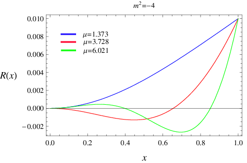
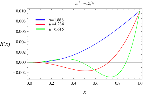
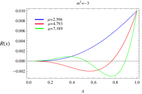
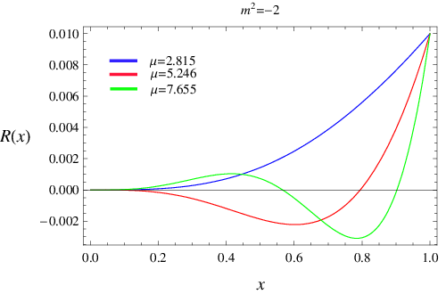
Fig.(2) shows the multiple marginally stable curves of the scalar fields 33 3 Note that we have transformed the scalar field to in coordinates. in coordinates for various . Take the plot of for example, the first three lowest-lying chemical potentials are in the sequence . We find that the values of ’s obtained from the “shooting” method are perfectly consistent with the ’s in Table (1) derived from the “marginally stable modes” method. The blue line is for the minimal value of . It starts from a very small initial value at the tip and then monotonically decrease to zero at the infinite boundary . There are no other intersecting points between the blue line and the axis. This is the reason we call the mode with of node . For the red and green lines, they are related to and respectively. The red line has one intersecting point with axis while the green line has two. Therefore, as we have mentioned above, we can call the two modes with nodes and respectively. However, the red and green lines are expected to be unstable, because radial oscillations in -direction of will cost energy [18]. In addition, the arguments above are also appropriate for other diagrams in Fig.(2).
3 P-wave perturbations
In this section we extend our work to study an AdS soliton with p-wave vector fields. We consider a five-dimensional SU(2) Einstein-Yang-Mills theory with a negative cosmological constant following [22] . The action is
| (22) |
where is the field strength of the SU(2) gauge theory and . are the indices of the SU(2) Lie algebra generator. are the components of the mixed-valued gauge fields , where are the generators of the SU(2) Lie algebra with commutation relation . And is a totally antisymmetric tensor with .
As a consistent solution of the system, in the probe limit, the background of the metric can also be an AdS soliton solution like (1) (We have scaled ),
| (23) |
where we have set .
We adopt the ansatz for the gauge field as [18]
| (24) |
Note that in order to consider the QNMs of the vector field, we have assumed depends on and . In this ansatz, the gauge boson with nonzero component along -direction is charged under . According to AdS/CFT dictionary, is dual to the chemical potential in the boundary field theory while is dual to the -component of some charged vector operator . The condensation of will spontaneously break the U(1)3 gauge symmetry and induce the phenomena of superconducting on the boundary field theory.
Define , the EoMs for and in the coordinate are
| (25) | |||
| (26) |
where a prime denotes the derivative with respect to . A simple solution is that and which corresponds to an neutral AdS soliton with a constant electric potential.
In order to find the marginally stable modes of , we can follow the steps in the previous section. Eq.(26) can be transformed to
| (27) |
where, the coefficient functions are
| (28) | |||||
| (29) | |||||
| (30) |
Polynomially expand these three coefficient functions to a finite order and to an infinite order, such as
| (31) | |||||
| (32) |
where is a finite integer. Substitute (32) and (31) into Eq.(27) we reach a recursion relation as Eqs.(16) and (17) in the previous section. The solutions of can be derived by requiring .
In the practical numerical calculations, we take the order of the expansion of to be . Notice again that in the potential (30) and are symmetric. Using the trick we have adopted in the preceding section, we can easily find the marginally stable modes when . The first three lowest-lying critical chemical potentials are
| (33) |
The minimal critical chemical potential is in perfect agreement with the results in [10, 13].
In order to study the behavior of the field , we should first know the boundary conditions for and then make use of the “shooting” method to numerically calculate it. Notice again that we still assume the electric field here. At the tip, behaves as
| (34) |
while
| (35) |
at the infinite boundary. In the following calculation we will set in order not to source the field theory on the boundary.

We can see from Fig.(3) that there are multiple marginally stable curves corresponding to different critical chemical potentials. The blue line is related to the minimal value which is obtained from the “shooting” method. Once again, we find that this critical value of chemical potential is identical to the one derived from the “marginally stable modes” method. In addition, other values of are also consistent. From what we have learned in the last section, the blue line corresponds to the modes of node while red and green lines are related to the modes of node and respectively. However, the last two modes, i.e., and are unstable due to the cost of energy.
4 Discussions and Conclusions
In this paper, we have studied the marginally stable modes for the s-wave and p-wave perturbations in AdS soliton background with a constant electric potential. At some critical chemical potentials, the marginally stable modes, i.e. will arise. The importance of the marginally stable modes is that they can reveal the instabilities of the background which in our paper means that the neutral AdS soliton will become unstable to develop charged scalar (vector) “hairs” in this AdS soliton background. Although the detailed phase transitions cannot be seen in the study of QNMs, it actually has been announced in the previous works [6, 9, 10] by the study of thermodynamics such as the free energy. This phase transition in the gravity side will map to an insulator/superconductor phase transition on the boundary field theory.
Despite that we do not exactly know the phase structures through the marginally stable modes, they can actually indicate the onset of the phase transition. This has been argued by Gubser in studying the holographic superconductor phase transitions [2, 18]. In particular, marginally stable modes can be obtained by studying the QNMs of the perturbations. The widely used method to study QNMs in asymptotically AdS spacetime was Horowitz and Hubeny’s method [17]. In this paper, we have adopted this method to find that at some critical chemical potentials, there indeed appeared the marginally stable modes. These critical chemical potentials were in good agreement with those obtained from the previous studies [6, 10, 13]. We also took advantage of the “shooting” method to numerically plot the behaviors of the scalar (vector) fields in the radial direction. Therefore, one can intuitively see the “nodes” of the marginally stable modes. In addition to the modes of the minimal critical chemical potentials, we also studied other less lowest-lying marginally stable modes by both methods. We asserted that these less lowest-lying marginally stable modes are unstable because the oscillations of the scalar (vector) fields in radial direction will cost energy.
Acknowledgements
We would like to thank Hong-Bo Zhang for his indispensable help. HFL would be very grateful for the hospitalities of the members in the Institute of Theoretical Physics, Chinese Academy of Sciences. This work was supported in part by the National Natural Science Foundation of China (No. 10821504, No. 10975168, No.11035008 and No.11075098), and in part by the Ministry of Science and Technology of China under Grant No. 2010CB833004.
References
- [1] J. M. Maldacena, “The large N limit of superconformal field theories and supergravity,” Adv. Theor. Math. Phys. 2, 231 (1998) [Int. J. Theor. Phys. 38, 1113 (1999)] [arXiv:hep-th/9711200].
- [2] S. S. Gubser, “Breaking an Abelian gauge symmetry near a black hole horizon,” Phys. Rev. D 78, 065034 (2008) [arXiv:0801.2977 [hep-th]].
- [3] S. A. Hartnoll, C. P. Herzog and G. T. Horowitz, “Building a Holographic Superconductor,” Phys. Rev. Lett. 101, 031601 (2008) [arXiv:0803.3295 [hep-th]].
- [4] S. A. Hartnoll, “Lectures on holographic methods for condensed matter physics,” Class. Quant. Grav. 26, 224002 (2009) [arXiv:0903.3246 [hep-th]].
- [5] S. Weinberg, “Superconductivity For Particular Theorists,” Prog. Theor. Phys. Suppl. 86, 43 (1986).
- [6] T. Nishioka, S. Ryu, T. Takayanagi, “Holographic Superconductor/Insulator Transition at Zero Temperature,” JHEP 1003, 131 (2010). [arXiv:0911.0962 [hep-th]].
- [7] G. T. Horowitz, R. C. Myers, “The AdS / CFT correspondence and a new positive energy conjecture for general relativity,” Phys. Rev. D59, 026005 (1998). [hep-th/9808079].
- [8] E. Witten, “Anti-de Sitter space, thermal phase transition, and confinement in gauge theories,” Adv. Theor. Math. Phys. 2, 505-532 (1998). [hep-th/9803131].
- [9] G. T. Horowitz, B. Way, “Complete Phase Diagrams for a Holographic Superconductor/Insulator System,” JHEP 1011, 011 (2010). [arXiv:1007.3714 [hep-th]].
- [10] A. Akhavan, M. Alishahiha, “P-Wave Holographic Insulator/Superconductor Phase Transition,” [arXiv:1011.6158 [hep-th]].
- [11] P. Basu, F. Nogueira, M. Rozali, J. B. Stang and M. Van Raamsdonk, “Towards A Holographic Model of Color Superconductivity,” arXiv:1101.4042 [hep-th].
- [12] Y. Brihaye and B. Hartmann, “Holographic superfluid/fluid/insulator phase transitions in 2+1 dimensions,” arXiv:1101.5708 [hep-th].
- [13] R. G. Cai, H. F. Li and H. Q. Zhang, “Analytical Studies on Holographic Insulator/Superconductor Phase Transitions,” arXiv:1103.5568 [hep-th].
- [14] K. D. Kokkotas and B. G. Schmidt, “Quasinormal modes of stars and black holes,” Living Rev. Rel. 2, 2 (1999) [arXiv:gr-qc/9909058].
- [15] E. Berti, V. Cardoso and A. O. Starinets, “Quasinormal modes of black holes and black branes,” Class. Quant. Grav. 26, 163001 (2009) [arXiv:0905.2975 [gr-qc]].
- [16] R. A. Konoplya and A. Zhidenko, “Quasinormal modes of black holes: From astrophysics to string theory,” arXiv:1102.4014 [gr-qc].
- [17] G. T. Horowitz and V. E. Hubeny, “Quasinormal modes of AdS black holes and the approach to thermal Phys. Rev. D 62, 024027 (2000) [arXiv:hep-th/9909056].
- [18] S. S. Gubser and S. S. Pufu, “The Gravity dual of a p-wave superconductor,” JHEP 0811, 033 (2008) [arXiv:0805.2960 [hep-th]].
- [19] J. Shen, B. Wang, C. Y. Lin, R. G. Cai and R. K. Su, “The phase transition and the Quasi-Normal Modes of black Holes,” JHEP 0707, 037 (2007) [arXiv:hep-th/0703102].
- [20] X. He, B. Wang, R. G. Cai and C. Y. Lin, “Signature of the black hole phase transition in quasinormal modes,” Phys. Lett. B 688, 230 (2010) [arXiv:1002.2679 [hep-th]].
- [21] I. R. Klebanov and E. Witten, “AdS / CFT correspondence and symmetry breaking,” Nucl. Phys. B 556 (1999) 89 [arXiv:hep-th/9905104].
- [22] S. S. Gubser, “Colorful horizons with charge in anti-de Sitter space,” Phys. Rev. Lett. 101, 191601 (2008). [arXiv:0803.3483 [hep-th]].