跳到论文正文
W Papers独立论文阅读器 arXiv:1105.4956 论文正文 计算阅读时间 · 0%
引用这篇论文根据当前论文元数据生成,正式投稿前建议核对。


License: arXiv.org perpetual non-exclusive license
arXiv:1105.4956v1 [math-ph] 25 May 2011

On the stability of the massive scalar field in Kerr space-time

Horst Reinhard Beyer Affiliation: MPI for Gravitational Physics Affiliation: Am Muehlenberg 1 Affiliation: D-14476 Golm Affiliation: Germany Affiliation: Email: horst@aei.mpg.de
August 24, 2026
Abstract

The current early stage in the investigation of the stability of the Kerr metric is characterized by the study of appropriate model problems. Particularly interesting is the problem of the stability of the solutions of the Klein-Gordon equation, describing the propagation of a scalar field in the background of a rotating (Kerr-) black hole. Results suggest that the stability of the field depends crucially on its mass μ\mu. Among others, the paper provides an improved bound for μ\mu above which the solutions of the reduced, by separation in the azimuth angle in Boyer-Lindquist coordinates, Klein-Gordon equation are stable. Finally, it gives new formulations of the reduced equation, in particular, in form of a time-dependent wave equation that is governed by a family of unitarily equivalent positive self-adjoint operators. The latter formulation might turn out useful for further investigation. On the other hand, it is proved that from the abstract properties of this family alone it cannot be concluded that the corresponding solutions are stable.

1 Introduction

Kerr space-time is the only possible vacuum exterior solution of Einstein’s field equations describing a stationary, rotating, uncharged black hole with non-degenerate event horizon [31] and is expected to be the unique, stationary, asymptotically flat, vacuum space-time containing a non-degenerate Killing horizon [2]. Also, it is expected to be the asymptotic limit of the evolution of asymptotically flat vacuum data in general relativity.
An important step towards establishing the validity of these expectations is the proof of the stability of Kerr space-time. In comparison to Schwarzschild space-time, where linearized stability has been proved, this problem is complicated by a lower dimensional symmetry group and the absence of a Killing field that is everywhere time-like outside the horizon. For instance, the latter is reflected in the fact that energy densities corresponding to the Klein-Gordon field in a Kerr gravitational field have no definite sign. This absence complicates the application of methods from operator theory and of so called ‘‘energy methods’’ that are both employed in estimating the decay of solutions of hyperbolic partial differential equations.11 1 For the first, see, for instance, [5]. For the second, see, for instance, Chapter 22 of [27].
On the other hand, two facts are worth noting. For this, note that in the following any reference to coordinates implicitly assumes use of Boyer-Lindquist coordinates [8].
First, in addition to its Killing vector fields that generate one-parameter groups of symmetries (isometries), Kerr space-time admits a Killing tensor [33] that is unrelated to its symmetries. Initiated by his groundbreaking work [10] on the complete separability of the Hamilton-Jacobi equation in a Kerr background, Carter discovered that an operator that is induced by this Killing tensor commutes with the wave operator. On the other hand, Carter’s operator contains a second order time derivative [11]. An analogous operator has been found for the operator governing linearized gravitational perturbations of the Kerr geometry [20]. A recent study finds another such ‘symmetry operator’ which only contains a first order time derivative and commutes with a rescaled wave operator [7]. Differently to Carter’s operator, this operator is analogous to symmetry operators induced by one-parameter group of isometries of the metric, in that it induces a mapping in the data space that is compatible with time evolution, and therefore describes a true symmetry of the solutions. It is likely that an analogous operator can be found for a rescaling of the linearized operator governing gravitational perturbations of the Kerr geometry. In case of existence, it should facilitate the generalization to a Kerr background of the Regge-Wheeler-Zerilli-Moncrief (RWZM) decomposition of fields on a Schwarzschild background [30, 35, 26, 32, 28, 15] which in turn should greatly simplify the analysis of the stability of Kerr space-time.
Second, there is a Killing field that is time-like in an open neighborhood of the event horizon given by

ξ:=∂t+a2​M​r+∂φ,\xi:=\partial_{t}+\frac{a}{2Mr_{+}}\,\partial_{\varphi}\,\,, (1.0.1)

where ∂t,∂φ\partial_{t},\partial_{\varphi} are coordinate vector fields of Boyer-Lindquist coordinates corresponding to the coordinate time tt and the azimuthal angular coordinate φ\varphi, M>0M>0 is the mass of the black hole and a∈[0,M]a\in[0,M] its rotational parameter. Moreover, if

aM⩽33,\frac{a}{M}\leqslant\frac{\sqrt{3}}{3}\,\,, (1.0.2)

ξ\xi is time-like in the ergoregion, see Lemma 2.2. On the other hand, ∂t\partial_{t} itself is space-like in the ergoregion, null on the stationary limit surface and time-like outside. For these reasons, at least for aa satisfying (1.0.2), it might be possible to “join” energy inequalities belonging to the Killing fields by ξ\xi and ∂t\partial_{t}.
The discussion of the stability of the Kerr black hole is in its early stages. The first intermediate goal is the proof or disproof of its stability under “small” perturbations. As mentioned before, the linearized stability of the Schwarzschild metric has already been proved. In that case, by using the RWZM decomposition of fields in a Schwarzschild background, the question of the stability can be completely reduced to the question of the stability of the solutions of the wave equation on Schwarzschild space-time. For Kerr space-time, a similar reduction is not known. If such reduction exists, there is no guarantee that the relevant equation is the scalar wave equation. It is quite possible that such equation contains an additional (even positive) potential term that, similar to the potential term introduced by a mass of the field, could result in instability of the solutions. Second, an instability of a massive scalar field in a Kerr background could indicate instability of the metric against perturbations by matter which generically has mass. If this were the case, even a proof of the stability of Kerr space-time could turn out as a purely mathematical exercise with little relevance for general relativity. Currently, the main focus is the study of the stability of the solutions of the Klein-Gordon field on a Kerr background with the hope that the results lead to insight into the problem of linearized stability. Although the results of this paper also apply to the case that μ=0\mu=0, its main focus is the case of Klein-Gordon fields of mass μ>0\mu>0.
Quite differently from the case of a Schwarzschild background, the results for these test cases suggest an asymmetry between the cases μ=0\mu=0 and μ≠0\mu\neq 0. In the case of the wave equation, i.e., μ=0\mu=0, results point to the stability of the solutions [34, 16, 12, 1, 23, 24], whereas for μ≠0\mu\neq 0, there are a number of results pointing in the direction of instability of the solutions under certain conditions [13, 14, 36, 17, 22, 9, 19].
In particular, unstable modes were found by the numerical investigations by Furuhashi and Nambu for μ​M∼1\mu M\sim 1 and (a/M)=0.98(a/M)=0.98, by Strafuss and Khanna for μ​M∼1\mu M\sim 1 and (a/M)=0.9999(a/M)=0.9999 and by Cardoso and Yoshida for μ​M⩽1\mu M\leqslant 1 and 0.98⩽(a/M)<10.98\leqslant(a/M)<1. The analytical study by Hod and Hod finds unstable modes for μ​M∼1\mu M\sim 1 with a growth rate which is four orders of magnitude larger than previous estimates. On the other hand, [3] proves that the restrictions of the solutions of the separated, in the azimuthal coordinate, Klein-Gordon field (RKG) are stable for

μ⩾|m|​a2​M​r+​1+2​Mr++a2r+2.\mu\geqslant\frac{|m|a}{2Mr_{+}}\sqrt{1+\frac{2M}{r_{+}}+\frac{a^{2}}{r_{+}^{2}}}\,\,. (1.0.3)

Here m∈ℤm\in{\mathbb{Z}} is the ‘azimuthal separation parameter’ and r+:=M+M2−a2r_{+}:=M+\sqrt{M^{2}-a^{2}}. So far, this has been the only mathematically rigorous result on the stability of the solutions of the RKG for μ>0\mu>0. This result contradicts the result of Zouros and Eardley, but is consistent with the other results above. In addition, there is the numerical result by Konoplya and Zhidenko, [25] which confirms the result of Beyer, but also finds no unstable modes of the RKG for μ​M≪1\mu M\ll 1 and μ​M∼1\mu M\sim 1.
Among others, this paper improves the estimate (1.0.3). It is proved that the solutions of the RKG are stable for μ\mu satisfying

μ⩾|m|​a2​M​r+​1+2​Mr+.\mu\geqslant\frac{|m|a}{2Mr_{+}}\sqrt{1+\frac{2M}{r_{+}}}\,\,.

Further, it gives new formulations for RKG, in particular, in form of a time-dependent wave equation that is governed by a family of unitarily equivalent positive self-adjoint operators. The latter might turn out useful in future investigations. On the other hand, it is proved that from the abstract properties of this family alone it cannot be concluded that the corresponding solutions are stable.
The remainder of the paper is organized as follows. Section 22 gives the geometrical setting of the discussion of the solutions of the RKG and a proof of the above mentioned property of the Killing field ξ\xi. Section 33 gives basic properties of operators read off from the equation, including some new results. These properties provide the basis for a formulation of the initial-value problem for the equation in Section 44 which is less dependent on methods from semigroups of operators than that of [3]. Section 44 also contains the improved result on the stability of the solutions of RKG, a formulation of the RKG in terms of a time-dependent wave equation and the above mentioned counterexample. Finally, the paper concludes with a discussion of the results and 22 appendices that contain proof of results that were omitted in the main text to improve the readability of the paper.

2 The Geometrical Setting

In Boyer-Lindquist coordinates22 2 If not otherwise indicated, the symbols t,r,θ,φt,r,\theta,\varphi denote coordinate projections whose domains will be obvious from the context. In addtion, we assume the composition of maps, which includes addition, multiplication and so forth, always to be maximally defined. For instance, the sum of two complex-valued maps is defined on the intersection of their domains. Finally, we use Planck units where the reduced Planck constant ℏ\hbar, the speed of light in vacuum cc, and the gravitational constant γ\gamma, all have the numerical value 11., (t,r,θ,φ):Ω→ℝ4(t,r,\theta,\varphi):\Omega\rightarrow{\mathbb{R}}^{4}, the Kerr metric gg is given by

g=gt​t​d​t⊗d​t+gt​φ​(d​t⊗d​φ+d​φ⊗d​t)+gr​r​d​r⊗d​r+gθ​θ​d​θ⊗d​θ+gφ​φ​d​φ⊗d​φ,\displaystyle g=g_{tt}\,dt\otimes dt+g_{t\varphi}(dt\otimes d\varphi+d\varphi\otimes dt)+g_{rr}\,dr\otimes dr+g_{\theta\theta}\,d\theta\otimes d\theta+g_{\varphi\varphi}\,d\varphi\otimes d\varphi\,\,,

where

gt​t:=1−2​M​rΣ,gt​φ:=2​M​a​r​sin2⁡θΣ,gr​r:=−ΣΔ,gθ​θ:=−Σ,\displaystyle g_{tt}:=1-\frac{2Mr}{\Sigma}\,\,,\,\,g_{t\varphi}:=\frac{2Mar\sin^{2}\!\theta}{\Sigma}\,\,,\,\,g_{rr}:=-\frac{\Sigma}{\Delta}\,\,,\,\,g_{\theta\theta}:=-\Sigma\,\,,
gφ​φ:=−Δ​Σ¯Σ​sin2⁡θ,\displaystyle g_{\varphi\varphi}:=-\frac{\Delta\overline{\Sigma}}{\Sigma}\sin^{2}\!\theta\,\,,

MM is the mass of the black hole, a∈[0,M]a\in[0,M] is the rotational parameter and

Δ:=r2−2​M​r+a2,Σ:=r2+a2​cos2⁡θ,\displaystyle\Delta:=r^{2}-2Mr+a^{2}\,\,,\,\,\Sigma:=r^{2}+a^{2}\cos^{2}\!\theta\,\,,
Σ¯:=(r2+a2)​Σ+2​M​a2​r​sin2⁡θΔ=(r2+a2)2Δ−a2​sin2⁡θ=Σ+2​M​r+4​M2​r2Δ,\displaystyle\overline{\Sigma}:=\frac{(r^{2}+a^{2})\Sigma+2Ma^{2}r\sin^{2}\!\theta}{\Delta}=\frac{(r^{2}+a^{2})^{2}}{\Delta}-a^{2}\sin^{2}\!\theta=\Sigma+2Mr+\frac{4M^{2}r^{2}}{\Delta}\,\,,
r+:=M+M2−a2,r−:=M−M2−a2,\displaystyle r_{+}:=M+\sqrt{M^{2}-a^{2}}\,\,,\,\,r_{-}:=M-\sqrt{M^{2}-a^{2}}\,\,,\,\,
Ω:=ℝ×(r+,∞)×(0,π)×(−π,π).\displaystyle\Omega:={\mathbb{R}}\times(r_{+},\infty)\times(0,\pi)\times(-\pi,\pi)\,\,.

In these coordinates, the reduced Klein-Gordon equation corresponding to m∈ℤm\in{\mathbb{Z}}, governing solutions ψ:Ω→ℂ\psi:\Omega\rightarrow{\mathbb{C}} of the form

ψ⁡(t,r,θ,φ)=exp⁡(i​m​φ)​u​(t,r,θ),\psi(t,r,\theta,\varphi)=\exp(im\varphi)\,u(t,r,\theta)\,\,,

where u:Ωs→ℂu:\Omega_{s}\rightarrow{\mathbb{C}},

Ωs:=(r+,∞)×(0,π),\Omega_{s}:=(r_{+},\infty)\times(0,\pi)\,\,,

for all t∈ℝt\in{\mathbb{R}}, φ∈(−π,π)\varphi\in(-\pi,\pi), (r,θ)∈Ωs(r,\theta)\in\Omega_{s}, is given by

∂2u∂t2+i​b​∂u∂t+Dr​θ2​u=0,\displaystyle\frac{\partial^{2}u}{\partial t^{2}}+ib\,\frac{\partial u}{\partial t}+D^{2}_{r\theta}\,u=0\,\,, (2.0.1)

where

b:=4​m​M​a​r△​Σ¯=4​m​M​a​r(r2+a2)2−a2​△​sin2⁡θ=4​m​M​a​r(r2+a2)​Σ+2​M​a2​r​sin2⁡θ,b:=\frac{4mMar}{\triangle\overline{\Sigma}}=\frac{4mMar}{(r^{2}+a^{2})^{2}-a^{2}\triangle\sin^{2}\theta}=\frac{4mMar}{(r^{2}+a^{2})\Sigma+2Ma^{2}r\sin^{2}\!\theta}\,\,,
Dr​θ2​f:=1Σ¯​(−∂∂r​△​∂∂r−m2​a2△−1sin⁡θ​∂∂θ​sin⁡θ​∂∂θ+m2sin2⁡θ+μ2​Σ)​f\displaystyle D^{2}_{r\theta}f:=\frac{1}{\overline{\Sigma}}\left(-\frac{\partial}{\partial r}\triangle\frac{\partial}{\partial r}-\frac{m^{2}a^{2}}{\triangle}-\frac{1}{\sin\theta}\,\frac{\partial}{\partial\theta}\sin\theta\,\frac{\partial}{\partial\theta}+\frac{m^{2}}{\sin^{2}\theta}+\mu^{2}\Sigma\right)f

for every f∈C2​(Ωs,ℂ)f\in C^{2}(\Omega_{s},{\mathbb{C}}) and μ≥0\mu\geq 0 is the mass of the field. In particular, note that bb defines a real-valued bounded function on Ωs\Omega_{s} which positive for m≥0m\geq 0 and negative for m≤0m\leq 0. For this reason, it induces a bounded self-adjoint (maximal multiplication) operator BB on the weighted L2L^{2}-space XX, see below, which is positive for m≥0m\geq 0 and negative for m≤0m\leq 0. Further, Dr​θ2D^{2}_{r\theta} is singular since the continuous extensions of the coeffcients of its highest (second) order radial derivative vanish on the horizon {r+}×[0,π]\{r_{+}\}\times[0,\pi].
In particular, the following proves that the Killing field

ξ:=∂t+a2​M​r+∂φ\xi:=\partial_{t}+\frac{a}{2Mr_{+}}\,\partial_{\varphi}

is time-like in an open neighborhood of the event horizon and time-like in the ergoregion if

aM⩽33.\frac{a}{M}\leqslant\frac{\sqrt{3}}{3}\,\,.

Proofs are given in Appendix 11.

Lemma 2.1.

Let M>0,a>0M>0,a>0. For every s∈ℝs\in{\mathbb{R}}, the function

g(∂t+s∂φ,∂t+s∂φ)g(\partial_{t}+s\,\partial_{\varphi},\partial_{t}+s\,\partial_{\varphi})

has a continuous extension to Ω¯s{\overline{\Omega}}_{s}. This extension is positive on ∂Ω¯s\partial{\overline{\Omega}}_{s} if and only if

s=a2​M​r+.s=\frac{a}{2Mr_{+}}\,\,.

Further,

ξ:=∂t+a2​M​r+∂φ\xi:=\partial_{t}+\frac{a}{2Mr_{+}}\,\partial_{\varphi}

is time-like precisely on

Ωe​2:=[2​M​r+−a2​sin2⁡θ−a​Δ1/2​sin⁡θ⁡(1+2​Mr−r−)]−1​((0,∞)).\Omega_{e2}:=\left[2Mr_{+}-a^{2}\sin^{2}\!\theta-a\,\Delta^{1/2}\sin\theta\left(1+\frac{2M}{r-r_{-}}\right)\right]^{-1}(\,(0,\infty)\,)\,\,.
Proof.

See Appendix 11. ∎

Lemma 2.2.

Let M>0,a>0M>0,a>0 and Ωe​1\Omega_{e1}, defined by

Ωe​1:=(a2​sin2⁡θ−△)−1​((0,∞)),\Omega_{e1}:=(a^{2}\sin^{2}\!\theta-\triangle)^{-1}((0,\infty))\,\,,

denote the ergoregion. If

aM≤33,\frac{a}{M}\leq\frac{\sqrt{3}}{3}\,\,, (2.0.2)

then

Ωe​1⊂Ωe​2.\Omega_{e1}\subset\Omega_{e2}\,\,.
Proof.

See Appendix 11. ∎

3 Basic Properties of Operators in the Equation

In a first step, we represent (2.0.1) as a differential equation for an unknown function uu with values in a Hilbert space. For this reason, we represent formal operators present in (2.0.1) as operators with well-defined domains in an appropriate Hilbert space and, subsequently, study basic properties of the resulting operators. Theorems 3.5, 3.6 provide new results.

Definition 3.1.

In the following, XX denotes the weighted L2L^{2}-space XX defined by

X:=LC2​(Ωs,Σ¯​sin⁡θ).X:=L_{C}^{2}\big(\Omega_{s}\,,\overline{\Sigma}\sin\theta\big)\,\,. (3.0.1)

Further, BB is the bounded linear self-adjoint operator on XX given by

B​f:=b​fBf:=bf (3.0.2)

for every f∈Xf\in X. Note that BB is positive for m≥0m\geq 0 and negative for m≤0m\leq 0.

Remark 3.2.

We note that, as consequence of the fact that B∈L⁡(X,X)B\in L(X,X) is self-adjoint, the operator

exp⁡((i​t/2)​B),\exp((it/2)B)\,\,,

where exp\exp denotes the exponential function on L⁡(X,X)L(X,X), see, e.g., Section 3.3 in [5], is unitary for every t∈ℝt\in{\mathbb{R}} and coincides with the maximal multiplication operator by the function exp⁡((i​t/2)​b)\exp((it/2)b).

Definition 3.3.

(Definition of A0A_{0})

  • (i)

    We define D⁡(A0)D(A_{0}) to consist of all f∈C2​(Ω¯s,ℂ)∩Xf\in C^{2}({\bar{\Omega}}_{s},{\mathbb{C}})\cap X satisfying the conditions a), b) and c):

    • a)

      Dr​θ2​f∈XD^{2}_{r\theta}f\in X,

    • b)

      there is R>0R>0 such that f⁡(r,θ)=0f(r,\theta)=0 for all r>Rr>R and θ∈Iθ:=(0,π)\theta\in I_{\theta}:=(0,\pi),

    • c)
      limr→r+∂f∂θ​(r,θ)=0\lim_{r\rightarrow r_{+}}\frac{\partial f}{\partial\theta}(r,\theta)=0

      for all θ∈Iθ\theta\in I_{\theta}.

  • (ii)

    For every f∈D⁡(A0)f\in D(A_{0}), we define

    A0​f:=Dr​θ2​f.A_{0}f:=D^{2}_{r\theta}f\,\,.
Lemma 3.4.

A0A_{0} is a densely-defined, linear, symmetric and essentially self-adjoint operator in XX. In addition, the closure A¯0{\bar{A}}_{0} of A0A_{0} is semibounded with lower bound

α:=−m2​a24​M2​r+2.\alpha:=-\frac{m^{2}a^{2}}{4M^{2}r_{+}^{2}}\,\,.
Proof.

See Lemma 22 and Theorem 44 in [7]. ∎

Theorem 3.5.

The span, DD, of all products

f⊗(Plm∘cos),f\otimes(P^{m}_{l}\circ\cos)\,\,,

where f∈C02​((r+,∞),ℂ)f\in C^{2}_{0}((r_{+},\infty),{\mathbb{C}}) and Plm:(−1,1)→ℝP^{m}_{l}:(-1,1)\rightarrow{\mathbb{R}} is the generalized Legendre polynomial corresponding to m∈ℤm\in{\mathbb{Z}} and l∈{|m|,|m|+1,…}l\in\{|m|,|m|+1,\dots\}, is a core for A¯0{\bar{A}}_{0}.

Proof.

For this, we use the notation of [7]. According to the proof of Theorem 4 of [7], the underlying sets of XX and OPENX¯:=L2​(Ωs,(r4/Δ)​sin⁡θ)){\bar{X}}:=L^{2}({\Omega}_{s},(r^{4}/\Delta)\sin\theta)) are equal; and the norms induced on the common set are equivalent, the maximal multiplication operator Tr4/(Δ​Σ¯)T_{r^{4}/(\Delta\overline{\Sigma})} by the function r4/(Δ​Σ¯)r^{4}/(\Delta\overline{\Sigma}) is a bijective bounded linear operator on XX that has a bounded linear inverse; the operator HH, related to A0A_{0} by

A0=Tr4/(Δ​Σ¯)​H,A_{0}=T_{r^{4}/(\Delta\overline{\Sigma})}H\,\,, (3.0.3)

is a densely-defined, linear, symmetric, semibounded and essentially self-adjoint operator in X¯{\bar{X}}, and DD is contained in the (coinciding) domains of A0A_{0} and HH. Further, it has been shown that (H−λ)​D(H-\lambda)D is dense in X¯{\bar{X}} for λ<β\lambda<\beta, where β:=−m2a2/r+4\beta:=-m^{2}a^{2}/r_{+}^{4} is a lower bound for HH. From this follows that DD is a core for the closure H¯{\bar{H}} of HH. For the proof, let f∈D⁡(H¯)f\in D(\bar{H}). Since (H−λ)​D(H-\lambda)D is dense in X¯{\bar{X}}, there is a sequence f1,f2,…f_{1},f_{2},\dots in DD such that

limν→∞(H−λ)​fν=(H¯−λ)​f.\lim_{\nu\rightarrow\infty}(H-\lambda)f_{\nu}=({\bar{H}}-\lambda)f\,\,.

Since H¯−λ{\bar{H}}-\lambda is bijective with a bounded inverse, the latter implies that f1,f2,…f_{1},f_{2},\dots is convergent to ff and also that

limν→∞H​fν=H¯​f.\lim_{\nu\rightarrow\infty}Hf_{\nu}={\bar{H}}f\,\,.

Hence, we conclude that H¯{\bar{H}} coincides with the closure of H|DH|_{D}. Since Tr4/(Δ​Σ¯),Tr4/(Δ​Σ¯)−1∈L⁡(X,X)T_{r^{4}/(\Delta\overline{\Sigma})},T_{r^{4}/(\Delta\overline{\Sigma})}^{-1}\in L(X,X), from the latter also follows that A¯0{\bar{A}}_{0} coincides with the closure of A0|DA_{0}|_{D}. ∎

Theorem 3.6.

The operator A¯0{\bar{A}}_{0} coincides with the Friedrichs extension of the restriction of A0A_{0} to C0∞​(Ωs,ℂ)C^{\infty}_{0}({\Omega}_{s},{\mathbb{C}}).

Proof.

As a consequence of Theorem 3 in [3], it follows that DD is contained in the domain of the Friedrichs extension AFA_{F} of the restriction of A0A_{0} to C0∞​(Ωs,ℂ)C^{\infty}_{0}({\Omega}_{s},{\mathbb{C}}) and that AF​f=A0​fA_{F}f=A_{0}f for every f∈Df\in D. In this connection, note that the addition of a multiple of the identity operator ‘does not affect’ the Friedrichs extension of an operator.33 3 I.e., if AA is a densely-defined, linear, symmetric and semibounded operator in some Hilbert space XX and γ∈ℝ\gamma\in{\mathbb{R}}, then the Friedrichs extension of A+γA+\gamma, (A+γ)F(A+\gamma)_{F}, and the sum of the Friedrichs extension of AA, AFA_{F}, and γ\gamma coincide, (A+γ)F=AF+γ(A+\gamma)_{F}=A_{F}+\gamma. Since DD is a core for A¯0{\bar{A}}_{0}, from this follows that AF⊃A¯0A_{F}\supset{\bar{A}}_{0} and hence, since AFA_{F} is in particular symmetric and A¯0{\bar{A}}_{0} is self-adjoint, that AF=A¯0A_{F}={\bar{A}}_{0}. ∎

Lemma 3.7.
𝒜:=A¯0+(1/4)​B2{\cal A}:={\bar{A}}_{0}+(1/4)\,B^{2}

is a densely-defined, linear and positive self-adjoint operator in XX.

Proof.

That 𝒜{\cal A} is a densely-defined, linear and self-adjoint operator in XX is a consequence of Theorem 3.4 and the Rellich-Kato theorem. For the latter, see e.g. Theorem X.12 in [29], Vol. II. The positivity of 𝒜{\cal A} is a simple consequence of the fact that

1Σ¯​(−m2​a2△+m2sin2⁡θ)+14​b2=m2​[△−a2​sin2⁡θ△​Σ¯​sin2⁡θ+4​M2​a2​r2(△​Σ¯)2]\displaystyle\frac{1}{\overline{\Sigma}}\left(-\,\frac{m^{2}a^{2}}{\triangle}+\frac{m^{2}}{\sin^{2}\theta}\right)+\frac{1}{4}\,b^{2}=m^{2}\left[\frac{\triangle-a^{2}\sin^{2}\theta}{\triangle\overline{\Sigma}\,\sin^{2}\theta}+\frac{4M^{2}a^{2}r^{2}}{(\,\triangle\overline{\Sigma}\,)^{2}}\right]
=m2(△​Σ¯)2​sin2⁡θ​[(△−a2​sin2⁡θ)​△​Σ¯+4​M2​a2​r2​sin2⁡θ]\displaystyle=\frac{m^{2}}{(\,\triangle\overline{\Sigma}\,)^{2}\sin^{2}\theta}\left[(\triangle-a^{2}\sin^{2}\theta)\,\triangle\overline{\Sigma}+4M^{2}a^{2}r^{2}\sin^{2}\!\theta\right]
=m2(△​Σ¯)2​sin2⁡θ​{(△−a2​sin2⁡θ)​[△⁡(Σ+2​M​r)+4​M2​r2]+4​M2​a2​r2​sin2⁡θ}\displaystyle=\frac{m^{2}}{(\,\triangle\overline{\Sigma}\,)^{2}\sin^{2}\theta}\left\{\,(\triangle-a^{2}\sin^{2}\theta)\,[\triangle(\Sigma+2Mr)+4M^{2}r^{2}]+4M^{2}a^{2}r^{2}\sin^{2}\!\theta\,\right\}
=m2△​Σ¯2​sin2⁡θ​[(△−a2​sin2⁡θ)​(Σ+2​M​r)+4​M2​r2]\displaystyle=\frac{m^{2}}{\triangle{\overline{\Sigma}}^{2}\sin^{2}\theta}\left[\,(\triangle-a^{2}\sin^{2}\theta)\,(\Sigma+2Mr)+4M^{2}r^{2}\right]
=m2△​Σ¯2​sin2⁡θ​[(Σ−2​M​r)​(Σ+2​M​r)+4​M2​r2]=m2​Σ2△​Σ¯2​sin2⁡θ≥0.\displaystyle=\frac{m^{2}}{\triangle{\overline{\Sigma}}^{2}\sin^{2}\theta}\left[\,(\Sigma-2Mr)\,(\Sigma+2Mr)+4M^{2}r^{2}\right]=\frac{m^{2}\,\Sigma^{2}}{\triangle{\overline{\Sigma}}^{2}\sin^{2}\theta}\geq 0\,\,.

∎

4 Formulation of an Initial Value Problem

In the following, we give an initial value formulation for equations of the type of (2.0.1) whose possibility is indicated by Theorem 4.114.11 in [4], see also Theorem 5.4.115.4.11 in [5]. Here, we give the details of such formulation, including abstract energy estimates that provide an independent basis for the estimate (1.0.3) and also for its improvement (4.0.5) below. Specialization of the abstract formulation to XX given by (3.0.1), A:=A¯0−CA:={\bar{A}}_{0}-C, BB given by (3.0.2) and C:=−(α+ε)C:=-(\alpha+\varepsilon) for some ε>0\varepsilon>0, provides an initial-value formulation for (2.0.1) on every open interval II of ℝ{\mathbb{R}} along with quantities that are conserved under time evolution. Note that in this case A+C=A¯0A+C={\bar{A}}_{0}. For convenience, the proofs of the following statements are given in the Appendix 22.

Assumption 4.1.

In the following, let (X,⟨|⟩)(X,\braket{\,|\,}) be a non-trivial complex Hilbert space and AA be a densely-defined, linear and strictly positive self-adjoint operator in XX.

Definition 4.2.

We denote by WA1W^{1}_{A} the complex Hilbert space44 4 WA1W^{1}_{A} may be regarded as a generalized Sobolev space. given by D⁡(A1/2)D(A^{1/2}) equipped with the scalar product ⟨|⟩1\braket{\,|\,}_{1}, defined by

⟨ξ|η⟩1:=⟨A1/2​ξ|A1/2​η⟩+⟨ξ|η⟩\braket{\xi|\eta}_{1}:=\braket{A^{1/2}\xi|A^{1/2}\eta}+\braket{\xi|\eta}

for every ξ,η∈D⁡(A1/2)\xi,\eta\in D(A^{1/2}), and induced norm ∥∥1\|\,\,\|_{1}.

Remark 4.3.

Note that, as a consequence of

‖ξ‖1=(‖A1/2​ξ‖2+‖ξ‖2)1/2≥‖ξ‖\|\xi\|_{1}=(\|A^{1/2}\xi\|^{2}+\|\xi\|^{2})^{1/2}\geq\|\xi\|

for every ξ∈D⁡(A1/2)\xi\in D(A^{1/2}), the imbedding WA1↪XW^{1}_{A}\hookrightarrow X is continuous.

Assumption 4.4.

Let B:D⁡(A1/2)→XB:D(A^{1/2})\rightarrow X be a symmetric linear operator in XX for which there are a∈[0,1)a\in[0,1) and b∈[0,∞)b\in[0,\infty) such that

‖B​ξ‖2≤a2​‖A1/2​ξ‖2+b2​‖ξ‖2\|B\xi\|^{2}\leq a^{2}\|A^{1/2}\xi\|^{2}+b^{2}\|\xi\|^{2}

for every ξ∈D⁡(A1/2)\xi\in D(A^{1/2}). Note that this implies that B∈L⁡(WA1,X)B\in L(W^{1}_{A},X). Further, let C∈L⁡(WA1,X)C\in L(W^{1}_{A},X) be a symmetric linear operator in XX and II be a non-empty open interval of ℝ{\mathbb{R}}.

Definition 4.5.

We define a solution space SIS_{I} to consist of all differentiable u:I→WA1u:I\rightarrow W^{1}_{A} with Ran​(u)⊂D​(A){\textrm{Ran}}(u)\subset D(A), such that u′:I→Xu^{\prime}:I\rightarrow X is differentiable and

(u′)′​(t)+i​B​u′​(t)+(A+C)​u​(t)=0(u^{\prime})^{\prime}(t)+iBu^{\prime}(t)+(A+C)u(t)=0 (4.0.1)

for every t∈It\in I.55 5 Note that the differentiability of uu implies that Ran​u′⊂WA1\textrm{Ran}u^{\prime}\subset W^{1}_{A}.

Note that (4.0.1) contains two types of derivatives. Every first derivative of uu is to be understood in the sense of derivatives of WA1W^{1}_{A}-valued functions, whereas every further derivative is to be understood in the sense of derivatives of XX-valued functions. Unless otherwise indicated, this convention is also adopted in the subsequent part of this section. On the other hand, since the imbedding WA1↪XW^{1}_{A}\hookrightarrow X is continuous, differentiability in the sense of WA1W^{1}_{A}-valued functions also implies differentiability in the sense of XX-valued functions, including agreement of the corresponding derivatives. In particular, every u∈SIu\in S_{I} also satisfies the equation

u′′​(t)+i​B​u′​(t)+(A+C)​u​(t)=0u^{\prime\prime}(t)+iBu^{\prime}(t)+(A+C)u(t)=0 (4.0.2)

for every t∈It\in I, where here all derivatives are to be understood in the sense of derivatives of XX-valued functions. Further, note that the assumptions on CC, in general, do not imply that A+CA+C is self-adjoint.

Remark 4.6.

According to Theorem 4.114.11 in [4], see also Theorem 5.4.115.4.11 in [5], for every t0∈It_{0}\in I, ξ∈D⁡(A)\xi\in D(A) and η∈WA1\eta\in W^{1}_{A}, there is a uniquely determined corresponding u∈SIu\in S_{I} such that u⁡(t0)=ξu(t_{0})=\xi and u′​(t0)=ηu^{\,\prime}(t_{0})=\eta. The proof uses methods from the theory of semigroups of operators. Independently, the uniqueness of such uu follows more elementary from energy estimates in part (iii) of the subsequent Lemma 4.7.

Parts (i) and (ii) of the subsequent Lemma 4.7 give a “conserved current” and a “conserved energy”, respectively, that are associated with solutions of (4.0.1). Part (iii) gives associated energy estimates, that, in particular, imply the uniqueness of the initial value problem for (4.0.1) stated in (iv).

Lemma 4.7.

Let u∈SIu\in S_{I} and t0∈It_{0}\in I. Then the following holds.

  • (i)

    If v∈SIv\in S_{I}, then ju,v:I→ℂj_{u,v}:I\rightarrow{\mathbb{C}}, defined by

    ju,v​(t):=⟨u⁡(t)|v′​(t)⟩−⟨u′​(t)|v⁡(t)⟩+i​⟨u⁡(t)|B​v​(t)⟩j_{u,v}(t):=\braket{u(t)|v^{\prime}(t)}-\braket{u^{\prime}(t)|v(t)}+i\braket{u(t)|Bv(t)}

    for every t∈It\in I, is constant.

  • (ii)

    The function Eu:I→ℝE_{u}:I\rightarrow{\mathbb{R}}, defined by

    Eu​(t):=‖u′​(t)‖2+⟨u⁡(t)|(A+C)​u​(t)⟩E_{u}(t):=\|u^{\prime}(t)\|^{2}+\braket{u(t)|(A+C)u(t)}

    for every t∈It\in I, is constant.

  • (iii)

    In addition, let A+CA+C be semibounded with lower bound γ∈ℝ\gamma\in{\mathbb{R}}. Then

    ‖u⁡(t2)‖≤{[‖u⁡(t1)‖+|Eu|1/2​(t2−t1)]​e|γ|1/2​(t2−t1)if ​γ<0,‖u⁡(t1)‖+Eu1/2​(t2−t1)if ​γ=0,(2​Eu/γ)1/2​(1−e−γ1/2​(t2−t1))+‖u⁡(t1)‖​e−γ1/2​(t2−t1)if ​γ>0,\|u(t_{2})\|\leq\begin{cases}[\,\|u(t_{1})\|+|E_{u}|^{1/2}(t_{2}-t_{1})\,]e^{|\gamma|^{1/2}\,(t_{2}-t_{1})}&\mbox{if }\gamma<0\,\,,\\ \|u(t_{1})\|+E_{u}^{1/2}\,(t_{2}-t_{1})&\mbox{if }\gamma=0\,\,,\\ (2E_{u}/\gamma)^{1/2}\left(1-e^{-\gamma^{1/2}(t_{2}-t_{1})}\right)+\|u(t_{1})\|e^{-\gamma^{1/2}(t_{2}-t_{1})}&\mbox{if }\gamma>0\,\,,\end{cases}

    for t1,t2∈It_{1},t_{2}\in I such that t1≤t2t_{1}\leq t_{2}.

  • (iv)

    In addition, let A+CA+C be semibounded. If v∈SIv\in S_{I} is such that

    u⁡(t0)=v⁡(t0),u′​(t0)=v′​(t0),u(t_{0})=v(t_{0})\,\,,\,\,u^{\prime}(t_{0})=v^{\prime}(t_{0})\,\,,

    then v=uv=u.

Proof.

See Appendix 22. ∎

Refer to caption
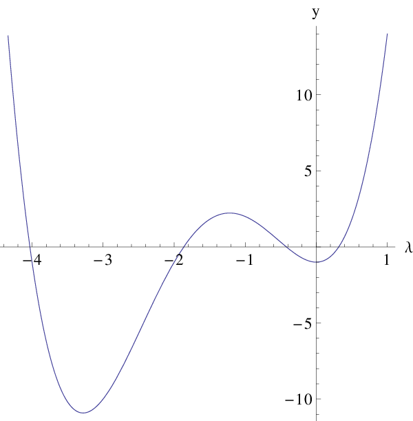
Fig. 1: Graph of (ℝ→L(X,X),λ↦A~−λB−λ2)({\mathbb{R}}\rightarrow L(X,X),\lambda\mapsto{\tilde{A}}-\lambda B-\lambda^{2}) for A~{\tilde{A}} and BB from Example 4.8.

The following example proves that it is possible that the energy assumes strictly negative values, but that the solutions of (4.0.1) are stable, i.e., that there are no exponentially growing solutions. This is different from the case of vanishing BB, where there are unstable solutions of (4.0.1) if and only if the energy assumes strictly negative values.

Example 4.8.

The example uses for the Hilbert space XX the space ℂ2{\mathbb{C}}^{2} equipped with the Euclidean scalar product, A~:=A+C{\tilde{A}}:=A+C and BB are the linear operators on ℂ2{\mathbb{C}}^{2} whose representations with respect to the canonical basis are given by the matrices

(100−1)​and​(3113),\begin{pmatrix}1&0\\ 0&-1\end{pmatrix}\,\,\textrm{and}\,\,\begin{pmatrix}3&1\\ 1&3\end{pmatrix}\,\,, (4.0.3)

respectively. An analysis shows that A~{\tilde{A}} and BB are bounded linear and self-adjoint operators in XX, A~{\tilde{A}} is semibounded, BB is positive and A~+(1/4)​B2{\tilde{A}}+(1/4)B^{2} is strictly positive. Further, A~{\tilde{A}} and BB do not commute. Finally, the operator polynomial (ℂ→L(X,X),λ↦A~−λB−λ2)({\mathbb{C}}\rightarrow L(X,X),\lambda\mapsto{\tilde{A}}-\lambda B-\lambda^{2}) has 44 distinct real eigenvalues. Therefore, in this case, there are no exponentially growing solutions of the corresponding equation (4.0.1). Fig 1 gives the graph of p:=(ℝ→L(X,X),λ↦det(A~−λB−λ2))=λ4+6λ3+8λ2−1p:=({\mathbb{R}}\rightarrow L(X,X),\lambda\mapsto\det({\tilde{A}}-\lambda B-\lambda^{2}))=\lambda^{4}+6\lambda^{3}+8\lambda^{2}-1 which suggests that there are precisely 44 distinct real roots. Indeed, we notice that

p⁡(−5)>0,p⁡(−4)<0,p⁡(−1)>0,p⁡(0)<0,p⁡(1)>0p(-5)>0\,\,,\,\,p(-4)<0\,\,,\,\,p(-1)>0\,\,,\,\,p(0)<0\,\,,\,\,p(1)>0

and hence that pp has real roots in the intervals (−5,−4)(-5,-4), (−4,−1)(-4,-1), (−1,0)(-1,0) and (0,1)(0,1). In addition, the value of the conserved energy EuE_{u} corrresponding to the solution uu of (4.0.1) with initial data u(0)=t(0,1)u(0)={\phantom{}}^{t}(0,1) and u′(0)=t(0,0)u^{\,\prime}(0)={\phantom{}}^{t}(0,0) is <0<0.

There are other possible definitions for the energy that is associated with solutions of (4.0.1). In cases of vanishing BB, such are usually not of further use. In the case of a nonvanishing BB, they can be useful as is the case for the RKG. In this case, the positivity of Es,uE_{s,u} for sufficiently large masses of the field and

s=m​a2​M​r+s=\frac{ma}{2Mr_{+}} (4.0.4)

provides a basis for (1.0.3) and its improvement (4.0.5) below.

Corollary 4.9.

Let s∈ℝs\in{\mathbb{R}} and u∈SIu\in S_{I}. Then, the function Es,u:I→ℝE_{s,u}:I\rightarrow{\mathbb{R}}, defined by

Es,u​(t):=‖u′​(t)+i​s​u​(t)‖2+⟨u⁡(t)|(A+C+s⁡(B−s))​u​(t)⟩E_{s,u}(t):=\|u^{\prime}(t)+isu(t)\|^{2}+\braket{u(t)|(A+C+s(B-s))u(t)}

for every t∈It\in I, is constant. If A+C+s⁡(B−s)A+C+s(B-s) is additionally semibounded with lower bound γ∈ℝ\gamma\in{\mathbb{R}}, then

‖u⁡(t2)‖≤{[‖u⁡(t1)‖+|Es,u|1/2​(t2−t1)]​e|γ|1/2​(t2−t1)if ​γ<0,‖u⁡(t1)‖+Es,u1/2​(t2−t1)if ​γ=0,(2​Es,u/γ)1/2​(1−e−γ1/2​(t2−t1))+‖u⁡(t1)‖​e−γ1/2​(t2−t1)if ​γ>0,\|u(t_{2})\|\leq\begin{cases}[\,\|u(t_{1})\|+|E_{s,u}|^{1/2}(t_{2}-t_{1})\,]e^{|\gamma|^{1/2}\,(t_{2}-t_{1})}&\mbox{if }\gamma<0\,\,,\\ \|u(t_{1})\|+E_{s,u}^{1/2}\,(t_{2}-t_{1})&\mbox{if }\gamma=0\,\,,\\ (2E_{s,u}/\gamma)^{1/2}\left(1-e^{-\gamma^{1/2}(t_{2}-t_{1})}\right)+\|u(t_{1})\|e^{-\gamma^{1/2}(t_{2}-t_{1})}&\mbox{if }\gamma>0\,\,,\end{cases}

for t1,t2∈It_{1},t_{2}\in I such that t1≤t2t_{1}\leq t_{2}.

Proof.

See Appendix 22. ∎

Theorem 4.10.

If there is s∈ℝs\in{\mathbb{R}} such that A+C+s⁡(B−s)A+C+s(B-s) is positive, then there are no exponentially growing solutions of (4.0.1).

Proof.

The statement is a direct consequence of Corollary 4.9 (or Theorem 4.174.17 (ii) in [4], see also Theorem 5.4.175.4.17 (ii) in [5]).

∎

Assumption 4.11.

In the following, we assume that XX is given by (3.0.1), A:=A¯0−CA:={\bar{A}}_{0}-C, BB is given by (3.0.2) and C:=−(α+ε)C:=-(\alpha+\varepsilon) for some ε>0\varepsilon>0.

Theorem 4.10 leads to an improvement of the estimate (1.0.3).

Theorem 4.12.

If

μ⩾|m|​a2​M​r+​1+2​Mr+,\mu\geqslant\frac{|m|a}{2Mr_{+}}\sqrt{1+\frac{2M}{r_{+}}}\,\,, (4.0.5)

then there are no exponentially growing solutions of (4.0.1).

Proof.

Let s∈ℝs\in{\mathbb{R}}. In the following, we estimate A¯0+s​B−s2{\bar{A}}_{0}+sB-s^{2}. For this, let f∈D⁡(A0)f\in D(A_{0}). Then

(A0+s​B−s2)​f=1Σ¯​(−∂∂r​△​∂∂r−1sin⁡θ​∂∂θ​sin⁡θ​∂∂θ+m2sin2⁡θ+Vs)​f,\displaystyle(A_{0}+sB-s^{2})f=\frac{1}{\overline{\Sigma}}\left(-\frac{\partial}{\partial r}\triangle\frac{\partial}{\partial r}-\frac{1}{\sin\theta}\,\frac{\partial}{\partial\theta}\sin\theta\,\frac{\partial}{\partial\theta}+\frac{m^{2}}{\sin^{2}\theta}+V_{s}\right)f\,\,,

where

Vs\displaystyle V_{s} :=−m2​a2△+μ2​Σ+s​4​m​M​a​r△−s2​Σ¯\displaystyle:=-\frac{m^{2}a^{2}}{\triangle}+\mu^{2}\Sigma+s\,\frac{4mMar}{\triangle}-s^{2}\,\overline{\Sigma}
=−(2​s​M​r−m​a)2Δ+(μ2−s2)​Σ−2​s2​M​r.\displaystyle\,\,=-\frac{(2sMr-ma)^{2}}{\Delta}+(\mu^{2}-s^{2})\Sigma-2s^{2}Mr\,\,.

First, we note that

m2sin2⁡θ≥m2.\frac{m^{2}}{\sin^{2}\theta}\geq m^{2}\,\,.

In the following, we assume that s=m​a/(2​M​r+)s=ma/(2Mr_{+}). Then

Vs​1:=−(2​s​M​r−m​a)2Δ=−(m​ar+)2+(m​ar+)2​2​M2−a2r−r−≥−m2.V_{s1}:=-\frac{(2sMr-ma)^{2}}{\Delta}=-\left(\frac{ma}{r_{+}}\right)^{2}+\left(\frac{ma}{r_{+}}\right)^{2}\,\frac{2\sqrt{M^{2}-a^{2}}}{r-r_{-}}\geq-m^{2}\,\,.

Further, we define

Vs​2:=(μ2−s2)​Σ−2​s2​M​r=(μ2−s2)​r2−2​s2​M​r+a2​(μ2−s2)​cos2⁡θ.V_{s2}:=(\mu^{2}-s^{2})\Sigma-2s^{2}Mr=(\mu^{2}-s^{2})r^{2}-2s^{2}Mr+a^{2}(\mu^{2}-s^{2})\cos^{2}\theta\,\,.

If μ≥|s|⋅[ 1+(2​M/r+)]1/2\mu\geq|s|\cdot[\,1+(2M/r_{+})\,]^{1/2}, then

Vs​2≥s2​2​Mr+​r2−2​s2​M​r+a2​(μ2−s2)​cos2⁡θ≥a2​(μ2−s2)​cos2⁡θ≥0.V_{s2}\geq s^{2}\,\frac{2M}{r_{+}}\,r^{2}-2s^{2}Mr+a^{2}(\mu^{2}-s^{2})\cos^{2}\theta\geq a^{2}(\mu^{2}-s^{2})\cos^{2}\theta\geq 0\,\,.

As a consequence,

1Σ¯​(m2sin2⁡θ+Vs)≥0.\frac{1}{\overline{\Sigma}}\left(\frac{m^{2}}{\sin^{2}\theta}+V_{s}\right)\geq 0\,\,.

Further, we conclude that

⟨f⊗(Pml∘cos)|(A0+sB−s2)(f⊗(Pml∘cos))⟩\displaystyle\braket{f\otimes(P^{m}_{l}\circ\cos)\,|\,(A_{0}+sB-s^{2})(f\otimes(P^{m}_{l}\circ\cos))}
≥∫Ωssinθ(f⊗(Plm∘cos))∗(−∂∂r△∂∂r−1sin⁡θ∂∂θsinθ∂∂θ)\displaystyle\geq\int_{\Omega_{s}}\sin\theta\,(f\otimes(P^{m}_{l}\circ\cos))^{*}\left(-\frac{\partial}{\partial r}\triangle\frac{\partial}{\partial r}-\frac{1}{\sin\theta}\,\frac{\partial}{\partial\theta}\sin\theta\,\frac{\partial}{\partial\theta}\right)
(f⊗(Plm∘cos))drdθ≥0\displaystyle\qquad\quad(f\otimes(P^{m}_{l}\circ\cos))\,drd\theta\geq 0

for every f∈C02​((r+,∞),ℂ)f\in C^{2}_{0}((r_{+},\infty),{\mathbb{C}}) and l∈{|m|,|m|+1,…}l\in\{|m|,|m|+1,\dots\}. Since DD is a core for A¯0{\bar{A}}_{0}, this implies that

A¯0+s​B−s2≥0.{\bar{A}}_{0}+sB-s^{2}\geq 0\,\,.

Hence the statement follows from Theorem 4.10. ∎

The following gives a connection of the operator A¯0+s​B−s2{\bar{A}}_{0}+sB-s^{2}, s∈ℝs\in{\mathbb{R}}, and the Killing field ∂t+s∂φ\partial_{t}+s\partial_{\varphi}. The corresponding proof is given in Appendix 22. This connection sheds light on the previous proof of the positivity of A¯0+s​B−s2{\bar{A}}_{0}+sB-s^{2} for s=m​a/(2​M​r+)s=ma/(2Mr_{+}) for sufficiently large μ\mu. Differently to gt​tg_{tt}, the term g(∂t+s∂φ,∂t+s∂φ)g(\partial_{t}+s\partial_{\varphi},\partial_{t}+s\partial_{\varphi}) is positive in a neighbourhood of the event horizon, but gradually turns negative away from the horizon. The latter is compensated by the mass term μ2​ρ\mu^{2}\rho for sufficiently large μ\mu.

Lemma 4.13.

Let s∈ℝs\in{\mathbb{R}} and ξ:=∂t+s∂φ\xi:=\partial_{t}+s\partial_{\varphi}. Then

[A0+m​s​B−(m​s)2]​f\displaystyle[\,A_{0}+msB-(ms)^{2}\,]f
=1gt​t[1−|g|∂r−|g|gr​r∂r+1−|g|∂θ−|g|gθ​θ∂θ]f+m2​g​(ξ,ξ)+μ2​ρ−gφ​φf.\displaystyle=\frac{1}{g^{tt}}\left[\frac{1}{\sqrt{-|g|}}\,\partial_{r}\sqrt{-|g|}\,g^{rr}\partial_{r}+\frac{1}{\sqrt{-|g|}}\,\partial_{\theta}\sqrt{-|g|}\,g^{\theta\theta}\partial_{\theta}\right]f+\frac{m^{2}g(\xi,\xi)+\mu^{2}\rho}{-g_{\varphi\varphi}}f\,\,.

for every f∈D⁡(A0)f\in D(A_{0}), where

ρ:=−[gt​t​gφ​φ−(gt​φ)2]=△​sin2⁡θ.\rho:=-[\,g_{tt}g_{\varphi\varphi}-(g_{t\varphi})^{2}\,]=\triangle\sin^{2}\!\theta\,\,.
Proof.

See Appendix 22. ∎

Subsequently, we rewrite (4.0.2) into an equivalent time-dependent wave equation that is governed by a family of unitarily equivalent positive self-adjoint operators. The latter equation might turn out useful for further investigation since only self-adjoint operators are involved. On the other hand, a subsequent example proves that from the abstract properties of this family alone it cannot be concluded that the solutions of the equation are stable.

Lemma 4.14.

Let BB be additionally bounded and u∈SIu\in S_{I}. Then, v:I→Xv:I\rightarrow X defined by

v⁡(t):=exp⁡((i​t/2)​B)​u​(t)v(t):=\exp((it/2)B)u(t)

for every t∈It\in I is twice differentiable in the sense of derivatives of XX-valued functions and satisfies

v′′​(t)+A⁡(t)​v​(t)=0v^{\prime\prime}(t)+A(t)v(t)=0 (4.0.6)

for every t∈It\in I, where

A⁡(t):=exp⁡((i​t/2)​B)​(A+C+14​B2)​exp⁡(−(i​t/2)​B)A(t):=\exp((it/2)B)\bigg(A+C+\frac{1}{4}\,B^{2}\bigg)\exp(-(it/2)B) (4.0.7)

for every t∈ℝt\in{\mathbb{R}}.

Proof.

See Appendix 22. ∎

The previous can be used to prove the stability of the solutions of (4.0.1) in particular cases where the operators A+CA+C and BB commute. Note that in these cases, there is a further conserved “energy” associated to the solutions of (4.0.1).

Theorem 4.15.

If, in addition, A+CA+C is self-adjoint and semibounded, BB is bounded, A+CA+C and BB commute, i.e.,

B∘(A+C)⊃(A+C)∘B,B\circ(A+C)\supset(A+C)\circ B\,\,,

and

A+C+14​B2,A+C+\frac{1}{4}\,B^{2}\,\,,

is positive, then there are no exponentially growing solutions of (4.0.1).

Proof.

The statement is a simple consequence of Lemma 4.14 and Lemma 4.7 (iii). ∎

Coming back to the statement of Lemma 4.14, for every t∈It\in I, the corresponding A⁡(t)A(t) is a densely-defined, linear and self-adjoint operator in XX, see, e.g., Lemma 7.1, in the Appendix. In particular, if A+C+(1/4)​B2A+C+(1/4)\,B^{2} is positive, A⁡(t)A(t) is positive, too. For instance, according to Lemma 3.7, this is true in the special case of the Klein-Gordon equation (2.0.1). Hence in such case it might be expected that (4.0.6) for u∈SIu\in S_{I} implies that ‖u‖\|u\| is not exponentially growing since this is the case if A⁡(t)=𝒜A(t)={\cal A} for every t∈It\in I, where 𝒜{\cal A} is a densely-defined, linear, positive self-adjoint operator in XX. In that case, uu is given by

u⁡(t)=cos⁡((t−t0)​𝒜1/2)​u​(t0)+sin⁡((t−t0)​𝒜1/2)𝒜1/2​u′​(t0)u(t)=\cos((t-t_{0}){\cal A}^{1/2})u(t_{0})+\frac{\sin((t-t_{0}){\cal A}^{1/2})}{{\cal A}^{1/2}}\,u^{\prime}(t_{0}) (4.0.8)

for all t0,t∈It_{0},t\in I, where cos⁡((t−t0)​𝒜1/2)\cos((t-t_{0}){\cal A}^{1/2}) and sin⁡((t−t0)​𝒜1/2/𝒜1/2)\sin((t-t_{0}){\cal A}^{1/2}/{\cal A}^{1/2}) denote the bounded linear operators that are associated by the functional calculus for 𝒜1/2{\cal A}^{1/2} to the restriction of cos((t−t0).idℝ)\cos((t-t_{0}).\textrm{id}_{\mathbb{R}}) and the restriction of the continuous extension of sin((t−t0).idℝ)/idℝ\sin((t-t_{0}).\textrm{id}_{\mathbb{R}})/\textrm{id}_{\mathbb{R}} to [0,∞)[0,\infty), respectively, to the spectrum of 𝒜1/2{\cal A}^{1/2} [5]. Note that the solutions (4.0.8) are in particular bounded if 𝒜{\cal A} is strictly positive. Unfortunately, this expectation is in general not true. A counterexample can be found already on the level of finite dimensional Hilbert spaces.
Refer to caption
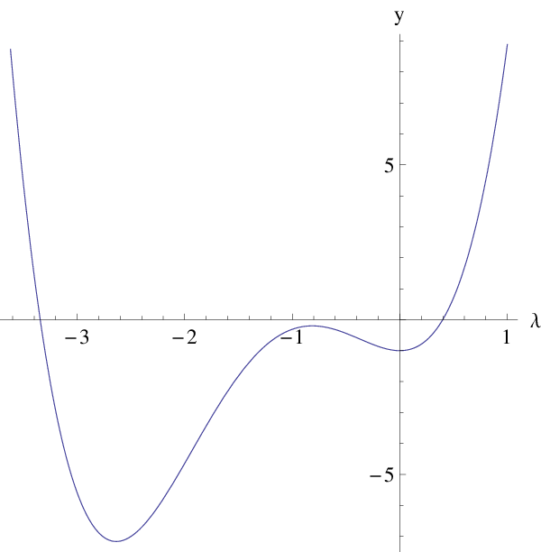
Fig. 2: Graph of (ℝ→L(X,X),λ↦A~−λB−λ2)({\mathbb{R}}\rightarrow L(X,X),\lambda\mapsto{\tilde{A}}-\lambda B-\lambda^{2}) for A~{\tilde{A}} and BB from Example 4.16.
Example 4.16.

The example uses for the Hilbert space XX the space ℂ2{\mathbb{C}}^{2} equipped with the Euclidean scalar product, A~:=A+C{\tilde{A}}:=A+C and BB are the linear operators on ℂ2{\mathbb{C}}^{2} whose representations with respect to the canonical basis are given by the matrices

(100−1)​and​(23/101123/10),\begin{pmatrix}1&0\\ 0&-1\end{pmatrix}\,\,\textrm{and}\,\,\begin{pmatrix}23/10&1\\ 1&23/10\end{pmatrix}\,\,, (4.0.9)

respectively. An analysis shows that A~{\tilde{A}} and BB are bounded linear and self-adjoint operators in XX, A~{\tilde{A}} is semibounded, BB is positive and A~+(1/4)​B2{\tilde{A}}+(1/4)B^{2} is even strictly positive. Further, A~{\tilde{A}} and BB do not commute. Finally, the operator polynomial (ℂ→L(X,X),λ↦A~−λB−λ2)({\mathbb{C}}\rightarrow L(X,X),\lambda\mapsto{\tilde{A}}-\lambda B-\lambda^{2}) has an eigenvalue with real part <0<0. Therefore, in this case, there is an exponentially growing solution of the corresponding equation (4.0.2) and hence also of (4.0.6). Note that in this case, the corresponding family of operators (4.0.7) consists of strictly positive bounded self-adjoint linear operators whose spectra are bounded from below by a common strictly positive real number. Fig 2 gives the graph of p:=(ℝ→L(X,X),λ↦det(A~−λB−λ2))=λ4+4.6λ3+4.29λ2−1p:=({\mathbb{R}}\rightarrow L(X,X),\lambda\mapsto\det({\tilde{A}}-\lambda B-\lambda^{2}))=\lambda^{4}+4.6\lambda^{3}+4.29\lambda^{2}-1 which suggests that there are precisely two distinct simple roots. Indeed, this is true. The proof proceeds by a discussion of the graph of pp using the facts that

p⁡(−4)>0,p⁡(−3)<0,p⁡(0)<0,p⁡(1)>0,p(-4)>0\,\,,\,\,p(-3)<0\,\,,\,\,p(0)<0\,\,,\,\,p(1)>0\,\,,

that the zeros of p′p^{\,\prime} are given by

(−69−1329)/40,(−69+1329)/40,  0(-69-\sqrt{1329}\,)/40\,\,,\,\,(-69+\sqrt{1329}\,)/40\,\,,\,\,0

and that

p⁡((−69+1329)/40)<0.p((-69+\sqrt{1329}\,)/40)<0\,\,.

Thus, (ℂ→L(X,X),λ↦det(A~−λB−λ2))({\mathbb{C}}\rightarrow L(X,X),\lambda\mapsto\det({\tilde{A}}-\lambda B-\lambda^{2})) has two distinct simple real roots and a pair of simple complex conjugate roots.

5 Discussion

The mathematical investigation of the stability of Kerr space-time has started, but is still in the phase of the study of relevant model equations in a Kerr background. The study of the solutions of the Klein-Gordon equation is expected to give important insight into the problem.
In the case of the wave equation, i.e., for the case of vanishing mass μ\mu of the scalar field, results point to the stability of the solutions. On the other hand, inspection of the reduced Klein-Gordon equation, 2.0.1, reveals that the case of μ>0\mu>0 originates from the case μ=0\mu=0 by the addition of a positive bounded potential term

μ2​ΣΣ¯\mu^{2}\,\frac{\Sigma}{\overline{\Sigma}}

to the equation. If there were no first order time derivative present in the equation, from this alone it would be easy to prove that the stability of the solutions of the wave equation implies the stability of the solutions of the Klein-Gordon equation for non-vanishing mass.
Even in the presence of such a derivative, it is hard to believe that the addition of such term causes instability. In particular, the energy estimates in Lemma 4.7, indicate a stabilizing influence of such a term. On the other hand, so far, there is no result that would allow to draw such conclusion.
The numerical results that indicate instability in the case μ≠0\mu\neq 0 make quite special assumptions on the values of the rotational parameter of the black hole that do not make them look very trustworthy. They could very well be numerical artefacts. Moreover, the numerical investigation by Konoplya et al., [25], does not find any unstable modes and contradicts all these investigations. Also the analytical results in this area are not accompanied by error estimates and therefore ultimately inconclusive. Still, apart from [36], all these results are consistent with the estimate on μ\mu in [3] and the improved estimate of this paper, above which the solutions of the reduced, by separation in the azimuth angle in Boyer-Lindquist coordinates, Klein-Gordon equation are stable.
It seems that the proof of the stability of the solutions of the wave equation in a Kerr background will soon be established. The question of the stability of the massive scalar field in a Kerr background is still an open problem, with only few rigorous results available, and displays surprising mathematical subtlety. In particular, in this case standard tools of theoretical physical investigation, including numerical investigations, seem too imprecise for analysis. Hence a rigorous mathematical investigation, like the one performed in this paper, seems to be enforced.

6 Appendix 1

In the following, we give the proofs of the Lemmatas 2.1 and 2.2 from Section 2.
Proof of Lemma 2.1.

Proof.

For this, let s∈ℝs\in{\mathbb{R}}. Then

g(∂t+s∂φ,∂t+s∂φ)=gt​t+2sgt​φ+s2gφ​φ\displaystyle g(\partial_{t}+s\,\partial_{\varphi},\partial_{t}+s\,\partial_{\varphi})=g_{tt}+2s\,g_{t\varphi}+s^{2}\,g_{\varphi\varphi}
=1−2​M​rΣ+4​s​M​a​r​sin2⁡θΣ−s2​Δ​Σ¯Σ​sin2⁡θ\displaystyle=1-\frac{2Mr}{\Sigma}+4s\,\frac{Mar\sin^{2}\!\theta}{\Sigma}-s^{2}\,\frac{\Delta\overline{\Sigma}}{\Sigma}\sin^{2}\!\theta
=ΔΣ+sin2⁡θΣ​[−a2+4​s​M​a​r−s2​(r2+a2)2+s2​a2​Δ​sin2⁡θ]\displaystyle=\frac{\Delta}{\Sigma}+\frac{\sin^{2}\!\theta}{\Sigma}\left[-a^{2}+4sMar-s^{2}(r^{2}+a^{2})^{2}+s^{2}a^{2}\Delta\sin^{2}\!\theta\right]
=ΔΣ+sin2⁡θΣ​[−(a−2​s​M​r)2+4​s2​M2​r2−s2​(r2+a2)2+a2​s2​Δ​sin2⁡θ]\displaystyle=\frac{\Delta}{\Sigma}+\frac{\sin^{2}\!\theta}{\Sigma}\left[-(a-2sMr)^{2}+4s^{2}M^{2}r^{2}-s^{2}(r^{2}+a^{2})^{2}+a^{2}s^{2}\Delta\sin^{2}\!\theta\,\right]
=ΔΣ+sin2⁡θΣ​[−(a−2​s​M​r)2−s2​Δ​(Δ+4​M​r)+a2​s2​Δ​sin2⁡θ]\displaystyle=\frac{\Delta}{\Sigma}+\frac{\sin^{2}\!\theta}{\Sigma}\left[-(a-2sMr)^{2}-s^{2}\Delta(\Delta+4Mr)+a^{2}s^{2}\Delta\sin^{2}\!\theta\,\right]
=ΔΣ−sin2⁡θΣ​[(a−2​s​M​r)2+s2​Δ​(Δ+4​M​r−a2​sin2⁡θ)]\displaystyle=\frac{\Delta}{\Sigma}-\frac{\sin^{2}\!\theta}{\Sigma}\left[(a-2sMr)^{2}+s^{2}\Delta(\Delta+4Mr-a^{2}\sin^{2}\!\theta)\,\right]

Hence g(∂t+s∂φ,∂t+s∂φ)g(\partial_{t}+s\,\partial_{\varphi},\partial_{t}+s\,\partial_{\varphi}) has a positive extension to the boundary of Ωs\Omega_{s} if and only if

s=a2​M​r+.s=\frac{a}{2Mr_{+}}\,\,.

In this case,

(a−2​s​M​r)2+s2​Δ​(Δ+4​M​r−a2​sin2⁡θ)\displaystyle(a-2sMr)^{2}+s^{2}\Delta(\Delta+4Mr-a^{2}\sin^{2}\!\theta)
=a2r+2​(r−r+)2+a24​M2​r+2​Δ​(Δ+4​M​r−a2​sin2⁡θ)\displaystyle=\frac{a^{2}}{r_{+}^{2}}\,(r-r_{+})^{2}+\frac{a^{2}}{4M^{2}r_{+}^{2}}\,\Delta(\Delta+4Mr-a^{2}\sin^{2}\!\theta)
=a24​M2​r+2​[ 4​M2​(r−r+)2+Δ⁡(Δ+4​M​r−a2​sin2⁡θ)]\displaystyle=\frac{a^{2}}{4M^{2}r_{+}^{2}}\left[\,4M^{2}(r-r_{+})^{2}+\Delta(\Delta+4Mr-a^{2}\sin^{2}\!\theta)\right]
=a2​Δ4​M2​r+2​[ 4​M2​r−r+r−r−+Δ+4​M​r−a2​sin2⁡θ]\displaystyle=\frac{a^{2}\Delta}{4M^{2}r_{+}^{2}}\left[\,4M^{2}\,\frac{r-r_{+}}{r-r_{-}}+\Delta+4Mr-a^{2}\sin^{2}\!\theta\right]

and hence

g(∂t+s∂φ,∂t+s∂φ)\displaystyle g(\partial_{t}+s\,\partial_{\varphi},\partial_{t}+s\,\partial_{\varphi})
=Δ4​M2​r+2​Σ​[4​M2​r+2−a2​sin2⁡θ⁡(4​M2​r−r+r−r−+Δ+4​M​r−a2​sin2⁡θ)]\displaystyle=\frac{\Delta}{4M^{2}r_{+}^{2}\Sigma}\left[4M^{2}r_{+}^{2}-a^{2}\sin^{2}\!\theta\left(4M^{2}\,\frac{r-r_{+}}{r-r_{-}}+\Delta+4Mr-a^{2}\sin^{2}\!\theta\right)\right]
=Δ4​M2​r+2​Σ​[(2​M​r+−a2​sin2⁡θ)2−a2​(r−r+)​sin2⁡θ⁡(4​M2r−r−+r−r−+4​M)]\displaystyle=\frac{\Delta}{4M^{2}r_{+}^{2}\Sigma}\left[(2Mr_{+}-a^{2}\sin^{2}\!\theta)^{2}-a^{2}(r-r_{+})\,\sin^{2}\!\theta\left(\,\frac{4M^{2}}{r-r_{-}}+r-r_{-}+4M\right)\right]
=Δ4​M2​r+2​Σ​[(2​M​r+−a2​sin2⁡θ)2−a2​Δ​sin2⁡θ​(1+2​Mr−r−)2].\displaystyle=\frac{\Delta}{4M^{2}r_{+}^{2}\Sigma}\left[(2Mr_{+}-a^{2}\sin^{2}\!\theta)^{2}-a^{2}\Delta\,\sin^{2}\!\theta\left(1+\,\frac{2M}{r-r_{-}}\right)^{2}\right]\,\,.

∎

Proof of Lemma 2.2.

Proof.

For this, let (r,θ)∈Ωe​1(r,\theta)\in\Omega_{e1}. Then

△⁡(r,θ)<a2​sin2⁡θ\triangle(r,\theta)<a^{2}\sin^{2}\!\theta

and

(2​M​r+−a2​sin2⁡θ)2−a2​Δ​(r,θ)​sin2⁡θ​(1+2​Mr−r−)2\displaystyle(2Mr_{+}-a^{2}\sin^{2}\!\theta)^{2}-a^{2}\Delta(r,\theta)\,\sin^{2}\!\theta\left(1+\,\frac{2M}{r-r_{-}}\right)^{2}
=a4​sin4⁡θ−[4​M​r++Δ⁡(r,θ)​(1+2​Mr−r−)2]​a2​sin2⁡θ+4​M2​r+2\displaystyle=a^{4}\sin^{4}\!\theta-\left[4Mr_{+}+\Delta(r,\theta)\left(1+\,\frac{2M}{r-r_{-}}\right)^{2}\right]a^{2}\sin^{2}\!\theta+4M^{2}r_{+}^{2}
>(Δ⁡(r,θ))2−[4​M​r++Δ⁡(r,θ)​(1+2​Mr−r−)2]​a2+4​M2​r+2\displaystyle>(\Delta(r,\theta))^{2}-\left[4Mr_{+}+\Delta(r,\theta)\left(1+\,\frac{2M}{r-r_{-}}\right)^{2}\right]a^{2}+4M^{2}r_{+}^{2}
=(Δ⁡(r,θ))2−a2​Δ​(r,θ)​(1+2​Mr−r−)2+4​M​r+​(M​r+−a2)\displaystyle=(\Delta(r,\theta))^{2}-a^{2}\Delta(r,\theta)\left(1+\,\frac{2M}{r-r_{-}}\right)^{2}+4Mr_{+}(Mr_{+}-a^{2})
=[Δ⁡(r,θ)−a22​(1+2​Mr−r−)2]2−a44​(1+2​Mr−r−)4+4​M​r+​(M​r+−a2)\displaystyle=\left[\Delta(r,\theta)-\frac{a^{2}}{2}\,\left(1+\,\frac{2M}{r-r_{-}}\right)^{2}\right]^{2}-\frac{a^{4}}{4}\,\left(1+\,\frac{2M}{r-r_{-}}\right)^{4}+4Mr_{+}(Mr_{+}-a^{2})
≥[Δ⁡(r,θ)−a22​(1+2​Mr−r−)2]2+4​[−a4​r+4(r+−r−)4+M​r+​(M​r+−a2)].\displaystyle\geq\left[\Delta(r,\theta)-\frac{a^{2}}{2}\,\left(1+\,\frac{2M}{r-r_{-}}\right)^{2}\right]^{2}+4\left[-\frac{a^{4}r_{+}^{4}}{(r_{+}-r_{-})^{4}}+Mr_{+}(Mr_{+}-a^{2})\right]\,\,.

Hence it follows that (r,θ)∈Ωe​2(r,\theta)\in\Omega_{e2} if

a4​r+4(r+−r−)4+a2​M​r+−M2​r+2\displaystyle\frac{a^{4}r_{+}^{4}}{(r_{+}-r_{-})^{4}}+a^{2}Mr_{+}-M^{2}r_{+}^{2}
=r+4(r+−r−)4​[a4+M​(r+−r−)4r+3​a2−M2​(r+−r−)4r+2]≤0.\displaystyle=\frac{r_{+}^{4}}{(r_{+}-r_{-})^{4}}\left[a^{4}+\frac{M(r_{+}-r_{-})^{4}}{r_{+}^{3}}\,a^{2}-\frac{M^{2}(r_{+}-r_{-})^{4}}{r_{+}^{2}}\right]\leq 0\,\,.

The latter is the case if and only if

a2≤2​M​r+1+1+4​r+4(r+−r−)4.\displaystyle a^{2}\leq\frac{2Mr_{+}}{1+\sqrt{1+\frac{4r_{+}^{4}}{(r_{+}-r_{-})^{4}}}}\,\,.

Further,

2​M​r+1+1+4​r+4(r+−r−)4≥M​r+1+r+2(r+−r−)2≥M21+M2M2−a2=M2​(M2−a2)2​M2−a2\displaystyle\frac{2Mr_{+}}{1+\sqrt{1+\frac{4r_{+}^{4}}{(r_{+}-r_{-})^{4}}}}\geq\frac{Mr_{+}}{1+\frac{r_{+}^{2}}{(r_{+}-r_{-})^{2}}}\geq\frac{M^{2}}{1+\frac{M^{2}}{M^{2}-a^{2}}}=\frac{M^{2}(M^{2}-a^{2})}{2M^{2}-a^{2}}
≥12​(M2−a2).\displaystyle\geq\frac{1}{2}\,(M^{2}-a^{2})\,\,.

Hence if

a2≤12​(M2−a2),a^{2}\leq\frac{1}{2}\,(M^{2}-a^{2})\,\,,

or, equivalently, if condition (2.0.2) is satisfied, it follows that (r,θ)∈Ωe​2(r,\theta)\in\Omega_{e2}. ∎

7 Appendix 2

In the following, we give the omitted proofs from Sections 3 and 4.
Proof of Lemma 4.7.

Proof.

‘(i)’: For this, let t∈It\in I and h∈ℝh\in{\mathbb{R}} such that t+h∈It+h\in I. Then

ju,v​(t+h)−ju,v​(t)h\displaystyle\frac{j_{u,v}(t+h)-j_{u,v}(t)}{h}
=h−1[⟨u⁡(t+h)|v′​(t+h)⟩−⟨u′​(t+h)|v⁡(t+h)⟩+i⟨u⁡(t+h)|B​v​(t+h)⟩\displaystyle=h^{-1}\left[\braket{u(t+h)|v^{\prime}(t+h)}-\braket{u^{\prime}(t+h)|v(t+h)}+i\braket{u(t+h)|Bv(t+h)}\right.
−⟨u⁡(t)|v′​(t)⟩+⟨u′​(t)|v⁡(t)⟩−i⟨u⁡(t)|B​v​(t)⟩]\displaystyle\left.\qquad\,\,\,\,\,\,\,\,-\braket{u(t)|v^{\prime}(t)}+\braket{u^{\prime}(t)|v(t)}-i\braket{u(t)|Bv(t)}\right]
=h−1[⟨u⁡(t+h)−u⁡(t)|v′​(t+h)⟩+⟨u⁡(t)|v′​(t+h)−v′​(t)⟩\displaystyle=h^{-1}\left[\braket{u(t+h)-u(t)|v^{\prime}(t+h)}+\braket{u(t)|v^{\prime}(t+h)-v^{\prime}(t)}\right.
−⟨u′​(t+h)|v⁡(t+h)−v⁡(t)⟩−⟨u′​(t+h)−u′​(t)|v⁡(t)⟩\displaystyle\left.\qquad\,\,\,\,\,\,\,\,-\braket{u^{\prime}(t+h)|v(t+h)-v(t)}-\braket{u^{\prime}(t+h)-u^{\prime}(t)|v(t)}\right.
+i⟨u⁡(t+h)−u⁡(t)|B​v​(t+h)⟩+i⟨B​u​(t)|v⁡(t+h)−v⁡(t)⟩].\displaystyle\left.\qquad\,\,\,\,\,\,\,\,+i\braket{u(t+h)-u(t)|Bv(t+h)}+i\braket{Bu(t)|v(t+h)-v(t)}\right]\,\,.

Hence it follows that ju,vj_{u,v} is differentiable in tt with derivative

ju,v′​(t)\displaystyle j_{u,v}^{\prime}(t) =⟨u⁡(t)|(v′)′​(t)⟩−⟨(u′)′​(t)|v⁡(t)⟩+i​⟨u′​(t)|B​v​(t)⟩+i​⟨B​u​(t)|v′​(t)⟩\displaystyle=\braket{u(t)|(v^{\prime})^{\prime}(t)}-\braket{(u^{\prime})^{\prime}(t)|v(t)}+i\braket{u^{\prime}(t)|Bv(t)}+i\braket{Bu(t)|v^{\prime}(t)}
=⟨u⁡(t)|(v′)′​(t)+i​B​v′​(t)⟩−⟨(u′)′​(t)+i​B​u′​(t)|v⁡(t)⟩\displaystyle=\braket{u(t)|(v^{\prime})^{\prime}(t)+iBv^{\prime}(t)}-\braket{(u^{\prime})^{\prime}(t)+iBu^{\prime}(t)|v(t)}
=−⟨u⁡(t)|(A+C)​v​(t)⟩+⟨(A+C)​u​(t)|v⁡(t)⟩=0.\displaystyle=-\braket{u(t)|(A+C)v(t)}+\braket{(A+C)u(t)|v(t)}=0\,\,.

From the latter, we conclude that the derivative of ju,vj_{u,v} vanishes and hence that ju,vj_{u,v} is a constant function.
‘(ii)’: For this, again, let t∈It\in I and h∈ℝh\in{\mathbb{R}} such that t+h∈It+h\in I. Further, let A~:=A+C\tilde{A}:=A+C. Then

Eu​(t+h)−Eu​(t)h\displaystyle\frac{E_{u}(t+h)-E_{u}(t)}{h}
=h−1​[⟨u′​(t+h)|u′​(t+h)⟩+⟨u⁡(t+h)|A~​u​(t+h)⟩−⟨u′​(t)|u′​(t)⟩−⟨u⁡(t)|A~​u​(t)⟩]\displaystyle=h^{-1}\left[\braket{u^{\prime}(t+h)|u^{\prime}(t+h)}+\braket{u(t+h)|{\tilde{A}}u(t+h)}-\braket{u^{\prime}(t)|u^{\prime}(t)}-\braket{u(t)|{\tilde{A}}u(t)}\right]
=h−1[⟨u′​(t+h)−u′​(t)|u′​(t+h)⟩+⟨u′​(t)|u′​(t+h)−u′​(t)⟩\displaystyle=h^{-1}\left[\braket{u^{\prime}(t+h)-u^{\prime}(t)|u^{\prime}(t+h)}+\braket{u^{\prime}(t)|u^{\prime}(t+h)-u^{\prime}(t)}\right.
+⟨u⁡(t+h)−u⁡(t)|A~​u​(t+h)⟩+⟨u⁡(t)|A~​(u​(t+h)−u​(t))⟩]\displaystyle\left.\qquad\,\,\,\,\,\,\,\,+\braket{u(t+h)-u(t)|{\tilde{A}}u(t+h)}+\braket{u(t)|{\tilde{A}}(u(t+h)-u(t))}\right]
=h−1[⟨u′​(t+h)−u′​(t)|u′​(t+h)⟩+⟨u′​(t)|u′​(t+h)−u′​(t)⟩\displaystyle=h^{-1}\left[\braket{u^{\prime}(t+h)-u^{\prime}(t)|u^{\prime}(t+h)}+\braket{u^{\prime}(t)|u^{\prime}(t+h)-u^{\prime}(t)}\right.
+⟨A1/2​(u⁡(t+h)−u⁡(t))|A1/2​u​(t+h)⟩+⟨u⁡(t+h)−u⁡(t)|C​u​(t+h)⟩\displaystyle\left.\qquad\,\,\,\,\,\,\,\,+\braket{A^{1/2}(u(t+h)-u(t))|A^{1/2}u(t+h)}+\braket{u(t+h)-u(t)|Cu(t+h)}\right.
+⟨A~​u​(t)|u⁡(t+h)−u⁡(t)⟩].\displaystyle\left.\qquad\,\,\,\,\,\,\,\,+\braket{{\tilde{A}}u(t)|u(t+h)-u(t)}\right]\,\,.

Hence it follows that EuE_{u} is differentiable in tt with derivative

⟨(u′)′​(t)|u′​(t)⟩+⟨u′​(t)|(u′)′​(t)⟩+⟨A1/2​u′​(t)|A1/2​u​(t)⟩+⟨u′​(t)|C​u​(t)⟩\displaystyle\braket{(u^{\prime})^{\prime}(t)|u^{\prime}(t)}+\braket{u^{\prime}(t)|(u^{\prime})^{\prime}(t)}+\braket{A^{1/2}u^{\prime}(t)|A^{1/2}u(t)}+\braket{u^{\prime}(t)|Cu(t)}
+⟨(A+C)​u​(t)|u′​(t)⟩\displaystyle+\braket{(A+C)u(t)|u^{\prime}(t)}
=−⟨i​B​u′​(t)+(A+C)​u​(t)|u′​(t)⟩−⟨u′​(t)|i​B​u′​(t)+(A+C)​u​(t)⟩\displaystyle=-\braket{iBu^{\prime}(t)+(A+C)u(t)|u^{\prime}(t)}-\braket{u^{\prime}(t)|iBu^{\prime}(t)+(A+C)u(t)}
+⟨u′​(t)|(A+C)​u​(t)⟩+⟨(A+C)​u​(t)|u′​(t)⟩\displaystyle\quad+\braket{u^{\prime}(t)|(A+C)u(t)}+\braket{(A+C)u(t)|u^{\prime}(t)}
=−⟨i​B​u′​(t)|u′​(t)⟩−⟨u′​(t)|i​B​u′​(t)⟩=0.\displaystyle=-\braket{iBu^{\prime}(t)|u^{\prime}(t)}-\braket{u^{\prime}(t)|iBu^{\prime}(t)}=0\,\,.

From the latter, we conclude that the derivative of EuE_{u} vanishes and hence that EuE_{u} is a constant function.
‘(iii)’: Since A+CA+C is semibounded with lower bound γ∈ℝ\gamma\in{\mathbb{R}},

⟨ξ|(A+C)​ξ⟩≥γ​‖ξ‖2\braket{\xi|(A+C)\xi}\geq\gamma\|\xi\|^{2}

for every ξ∈D⁡(A)\xi\in D(A). Hence it follows by (ii) that

‖u′​(t)‖2+γ​‖u⁡(t)‖2=Eu−(⟨u⁡(t)|(A+C)​u​(t)⟩−γ​‖u⁡(t)‖2)≤Eu\|u^{\prime}(t)\|^{2}+\gamma\|u(t)\|^{2}=E_{u}-(\braket{u(t)|(A+C)u(t)}-\gamma\|u(t)\|^{2})\leq E_{u} (7.0.1)

for every t∈ℝt\in{\mathbb{R}}. If γ=0\gamma=0, the latter implies that

‖u′​(t)‖≤Eu1/2\|u^{\prime}(t)\|\leq E_{u}^{1/2}

for every t∈It\in I. Hence it follows by weak integration in XX, e.g., see Theorem 3.2.53.2.5 in [5], that

‖u⁡(t2)−u⁡(t1)‖=‖∫(t1,t2)u′​(t)​𝑑t‖≤∫(t1,t2)‖u′​(t)‖​𝑑t≤Eu1/2​(t2−t1),\|u(t_{2})-u(t_{1})\|=\left\|\,\int_{(t_{1},t_{2})}u^{\,\prime}(t)\,dt\,\right\|\leq\int_{(t_{1},t_{2})}\|u^{\,\prime}(t)\|\,dt\leq E_{u}^{1/2}(t_{2}-t_{1})\,\,,

where t1,t2∈It_{1},t_{2}\in I are such that t1<t2t_{1}<t_{2}, and hence that

‖u⁡(t2)‖≤‖u⁡(t1)‖+Eu1/2​(t2−t1).\|u(t_{2})\|\leq\|u(t_{1})\|+E_{u}^{1/2}(t_{2}-t_{1})\,\,.

For the weak integration, note that the inclusion of WA1W^{1}_{A} into XX is continuous. If γ>0\gamma>0, it follows from (7.0.1) along with the parallelogram identity for elements of XX that

∥e−γ1/2​t(eγ1/2.idℝ.u)′(t)∥2=∥u′(t)+γ1/2u(t)∥2≤2(∥u′(t)∥2+∥γ1/2u(t)∥2)≤2Eu\displaystyle\|e^{-\gamma^{1/2}t}(e^{\gamma^{1/2}.{\textrm{id}}_{\mathbb{R}}}.u)^{\prime}(t)\|^{2}=\|u^{\prime}(t)+\gamma^{1/2}u(t)\|^{2}\leq 2(\,\|u^{\prime}(t)\|^{2}+\|\gamma^{1/2}u(t)\|^{2}\,)\leq 2E_{u}

and hence that

∥(eγ1/2.idℝ.u)′(t)∥≤(2Eu)1/2eγ1/2​t\|(e^{\gamma^{1/2}.{\textrm{id}}_{\mathbb{R}}}.u)^{\prime}(t)\|\leq(2E_{u})^{1/2}e^{\gamma^{1/2}t}

for t∈It\in I. Hence it follows by weak integration in XX that

∥eγ1/2​t2u(t2)−eγ1/2​t1u(t1)∥=‖∫(t1,t2)(eγ1/2.idℝ.u)′(t)dt‖\displaystyle\|e^{\gamma^{1/2}t_{2}}u(t_{2})-e^{\gamma^{1/2}t_{1}}u(t_{1})\|=\left\|\int_{(t_{1},t_{2})}(e^{\gamma^{1/2}.{\textrm{id}}_{\mathbb{R}}}.u)^{\prime}(t)\,dt\right\|
≤∫(t1,t2)∥(eγ1/2.idℝ.u)′(t)∥dt≤(2Eu/γ)1/2(eγ1/2​t2−eγ1/2​t1)\displaystyle\leq\int_{(t_{1},t_{2})}\|(e^{\gamma^{1/2}.{\textrm{id}}_{\mathbb{R}}}.u)^{\prime}(t)\|\,dt\leq(2E_{u}/\gamma)^{1/2}\left(e^{\gamma^{1/2}t_{2}}-e^{\gamma^{1/2}t_{1}}\right)

for all t1,t2∈It_{1},t_{2}\in I such that t1<t2t_{1}<t_{2}. The latter implies that

‖eγ1/2​t2​u​(t2)‖≤‖eγ1/2​t1​u​(t1)‖+(2​Eu/γ)1/2​(eγ1/2​t2−eγ1/2​t1).\|e^{\gamma^{1/2}t_{2}}u(t_{2})\|\leq\|e^{\gamma^{1/2}t_{1}}u(t_{1})\|+(2E_{u}/\gamma)^{1/2}\left(e^{\gamma^{1/2}t_{2}}-e^{\gamma^{1/2}t_{1}}\right)\,\,.

Hence

‖u⁡(t2)‖≤(2​Eu/γ)1/2​(1−e−γ1/2​(t2−t1))+e−γ1/2​(t2−t1)​‖u⁡(t1)‖.\|u(t_{2})\|\leq(2E_{u}/\gamma)^{1/2}\left(1-e^{-\gamma^{1/2}(t_{2}-t_{1})}\right)+e^{-\gamma^{1/2}(t_{2}-t_{1})}\|u(t_{1})\|\,\,.

If γ<0\gamma<0, it follows from (7.0.1) that

‖u′​(t)‖2≤Eu−γ​‖u⁡(t)‖2≤|Eu|+a​‖u⁡(t)‖2,\|u^{\prime}(t)\|^{2}\leq E_{u}-\gamma\|u(t)\|^{2}\leq|E_{u}|+a\,\|u(t)\|^{2}\,\,,

for every t∈It\in I, where a:=−γ>0a:=-\gamma>0. The latter implies that

‖u′​(t)‖≤|Eu|1/2+a1/2​‖u⁡(t)‖\|u^{\prime}(t)\|\leq|E_{u}|^{1/2}+a^{1/2}\,\|u(t)\|

for every t∈It\in I. Hence it follows by weak integration in XX that

‖u⁡(t2)−u⁡(t1)‖=‖∫(t1,t2)u′​(t)​𝑑t‖≤∫(t1,t2)‖u′​(t)‖​𝑑t\displaystyle\|u(t_{2})-u(t_{1})\|=\left\|\int_{(t_{1},t_{2})}u^{\,\prime}(t)\,dt\right\|\leq\int_{(t_{1},t_{2})}\|u^{\,\prime}(t)\|\,dt
≤|Eu|1/2​(t2−t1)+a1/2​∫(t1,t2)‖u⁡(t)‖​𝑑t,\displaystyle\leq|E_{u}|^{1/2}(t_{2}-t_{1})+a^{1/2}\int_{(t_{1},t_{2})}\|u(t)\|\,dt\,\,,

where t1,t2∈It_{1},t_{2}\in I are such that t1<t2t_{1}<t_{2}, and

‖u⁡(t2)‖≤‖u⁡(t1)‖+|Eu|1/2​(t2−t1)+a1/2​∫(t1,t2)‖u⁡(t)‖​𝑑t.\|u(t_{2})\|\leq\|u(t_{1})\|+|E_{u}|^{1/2}(t_{2}-t_{1})+a^{1/2}\int_{(t_{1},t_{2})}\|u(t)\|\,dt\,\,.

By help of the generalized Gronwall inequality from Lemma 3.1 in [18], from the latter we conclude that

‖u⁡(t2)‖≤[‖u⁡(t1)‖+|Eu|1/2​(t2−t1)]​ea1/2​(t2−t1)\|u(t_{2})\|\leq[\,\|u(t_{1})\|+|E_{u}|^{1/2}(t_{2}-t_{1})\,]e^{a^{1/2}(t_{2}-t_{1})}

for t1∈It_{1}\in I and t2∈It_{2}\in I such that t1<t2t_{1}<t_{2}.
‘(iv)’: For this, we define w:=v−uw:=v-u. Then ww is an element of SIS_{I} such that w⁡(t0)=w′​(t0)=0w(t_{0})=w^{\prime}(t_{0})=0. This implies that

Ew​(t):=‖w′​(t)‖2+⟨w⁡(t)|(A+C)​w​(t)⟩E_{w}(t):=\|w^{\prime}(t)\|^{2}+\braket{w(t)|(A+C)w(t)}

for every t∈It\in I is constant of value 00. Hence we conclude from (iii) that w⁡(t)=0Xw(t)=0_{X} for all t∈It\in I and therefore that v=uv=u.

∎

Proof of Corollary 4.9.

Proof.

We define v:I→WA1v:I\rightarrow W^{1}_{A} by

v⁡(t):=ei​s​t​u​(t)v(t):=e^{ist}u(t)

for every t∈It\in I. Then vv is differentiable with Ran​v⊂D⁡(A)\textrm{Ran}\,v\subset D(A) and also v′:I→Xv^{\prime}:I\rightarrow X is differentiable such that

v′​(t)=ei​s​t​[u′​(t)+i​s​u​(t)],(v′)′​(t)=ei​s​t​[(u′)′​(t)+2​i​s​u′​(t)−s2​u​(t)]v^{\prime}(t)=e^{ist}[u^{\prime}(t)+isu(t)]\,\,,\,\,(v^{\prime})^{\prime}(t)=e^{ist}[(u^{\prime})^{\prime}(t)+2isu^{\prime}(t)-s^{2}u(t)]

for every t∈It\in I. Further,

(v′)′​(t)+i⁡(B−2​s)​v′​(t)+(A+C+s​B−s2)​v​(t)\displaystyle(v^{\prime})^{\prime}(t)+i(B-2s)v^{\prime}(t)+(A+C+sB-s^{2})v(t)
=ei​s​t[(u′)′(t)+2isu′(t)−s2u(t)+i(B−2s)(u′(t)+isu(t))\displaystyle=e^{ist}[(u^{\prime})^{\prime}(t)+2isu^{\prime}(t)-s^{2}u(t)+i(B-2s)(u^{\prime}(t)+isu(t))
+(A+C+sB−s2)u(t)]\displaystyle\qquad\quad+(A+C+sB-s^{2})u(t)]
=ei​s​t[(u′)′(t)+2isu′(t)−s2u(t)+iBu′(t)−2isu′(t)−sBu(t)+2s2u(t)\displaystyle=e^{ist}[(u^{\prime})^{\prime}(t)+2isu^{\prime}(t)-s^{2}u(t)+iBu^{\prime}(t)-2isu^{\prime}(t)-sBu(t)+2s^{2}u(t)
+(A+C+sB−s2)u(t)]\displaystyle\qquad\quad+(A+C+sB-s^{2})u(t)]
=ei​s​t​[(u′)′​(t)+i​B​u′​(t)+(A+C)​u​(t)]=0\displaystyle=e^{ist}[(u^{\prime})^{\prime}(t)+iBu^{\prime}(t)+(A+C)u(t)]=0

for every t∈It\in I. Note that (X,A,B−2​s,C+s​B−s2)(X,A,B-2s,C+sB-s^{2}) satisfy Assumptions 4.1, 4.4. Hence it follows by Lemma 4.7 that the function Ev:I→ℝE_{v}:I\rightarrow{\mathbb{R}}, defined by

Ev​(t):=‖v′​(t)‖2+⟨v⁡(t)|(A+C+s​B−s2)​v​(t)⟩\displaystyle E_{v}(t):=\|v^{\prime}(t)\|^{2}+\braket{v(t)|(A+C+sB-s^{2})v(t)}
=‖u′​(t)+i​s​u​(t)‖2+⟨u⁡(t)|(A+C+s​B−s2)​u​(t)⟩\displaystyle=\|u^{\prime}(t)+isu(t)\|^{2}+\braket{u(t)|(A+C+sB-s^{2})u(t)}

for every t∈It\in I, is constant. If, in addition, A+C+s⁡(B−s)A+C+s(B-s) is semibounded with lower bound γ∈ℝ\gamma\in{\mathbb{R}}, then

‖v⁡(t2)‖≤{[‖v⁡(t1)‖+|Ev|1/2​(t2−t1)]​e|γ|1/2​(t2−t1)if ​γ<0,‖v⁡(t1)‖+Ev1/2​(t2−t1)if ​γ=0,(2​Ev/γ)1/2​(1−e−γ1/2​(t2−t1))+‖v⁡(t1)‖​e−γ1/2​(t2−t1)if ​γ>0,\|v(t_{2})\|\leq\begin{cases}[\,\|v(t_{1})\|+|E_{v}|^{1/2}(t_{2}-t_{1})\,]e^{|\gamma|^{1/2}\,(t_{2}-t_{1})}&\mbox{if }\gamma<0\,\,,\\ \|v(t_{1})\|+E_{v}^{1/2}\,(t_{2}-t_{1})&\mbox{if }\gamma=0\,\,,\\ (2E_{v}/\gamma)^{1/2}\left(1-e^{-\gamma^{1/2}(t_{2}-t_{1})}\right)+\|v(t_{1})\|e^{-\gamma^{1/2}(t_{2}-t_{1})}&\mbox{if }\gamma>0\,\,,\end{cases}

for t1,t2∈It_{1},t_{2}\in I such that t1≤t2t_{1}\leq t_{2}. ∎

Proof of Lemma 4.13.

Proof.

First, we notice that the only non-vanishing components of (ga​b)(a,b)∈{t,r,θ,φ}2(g^{ab})_{(a,b)\in\{t,r,\theta,\varphi\}^{2}} are given by

gt​t=Σ¯Σ,gt​φ=gφ​t=2​M​a​r△​Σ,gr​r=−△Σ,gθ​θ=−1Σ,\displaystyle g^{tt}=\frac{\overline{\Sigma}}{\Sigma}\,\,,\,\,g^{t\varphi}=g^{\varphi t}=\frac{2Mar}{\triangle\Sigma}\,\,,\,\,g^{rr}=-\frac{\triangle}{\Sigma}\,\,,\,\,g^{\theta\theta}=-\frac{1}{\Sigma}\,\,,\,\,
gφ​φ=−1△​sin2⁡θ​(1−2​M​rΣ).\displaystyle g^{\varphi\varphi}=-\frac{1}{\triangle\sin^{2}\!\theta}\,\left(1-\frac{2Mr}{\Sigma}\right)\,\,.

Further, we notice that

gt​t=−gφ​φρ,gt​φ=gt​φρ,gφ​φ=−gt​tρ,\displaystyle g^{tt}=-\frac{g_{\varphi\varphi}}{\rho}\,\,,\,\,g^{t\varphi}=\frac{g_{t\varphi}}{\rho}\,\,,\,\,g^{\varphi\varphi}=-\frac{g_{tt}}{\rho}\,\,,

where

ρ:=−[gt​t​gφ​φ−(gt​φ)2]=△​sin2⁡θ.\rho:=-[\,g_{tt}g_{\varphi\varphi}-(g_{t\varphi})^{2}\,]=\triangle\sin^{2}\!\theta\,\,.

Hence

1gt​t​□=\displaystyle\frac{1}{g^{tt}}\,\Box=\, ∂t2+2gt​φgt​t∂t∂φ+gφ​φgt​t∂φ2\displaystyle\partial_{t}^{2}+2\,\frac{g^{t\varphi}}{g^{tt}}\,\partial_{t}\partial_{\varphi}+\frac{g^{\varphi\varphi}}{g^{tt}}\,\partial_{\varphi}^{2}
+1gt​t[1−|g|∂r−|g|gr​r∂r+1−|g|∂θ−|g|gθ​θ∂θ]\displaystyle+\frac{1}{g^{tt}}\left[\frac{1}{\sqrt{-|g|}}\,\partial_{r}\sqrt{-|g|}\,g^{rr}\partial_{r}+\frac{1}{\sqrt{-|g|}}\,\partial_{\theta}\sqrt{-|g|}\,g^{\theta\theta}\partial_{\theta}\right]
=\displaystyle=\, ∂t2+2gt​φ−gφ​φ∂t∂φ−gt​t−gφ​φ∂φ2\displaystyle\partial_{t}^{2}+2\,\frac{g_{t\varphi}}{-g_{\varphi\varphi}}\,\partial_{t}\partial_{\varphi}-\frac{g_{tt}}{-g_{\varphi\varphi}}\,\partial_{\varphi}^{2}
+1gt​t[1−|g|∂r−|g|gr​r∂r+1−|g|∂θ−|g|gθ​θ∂θ].\displaystyle+\frac{1}{g^{tt}}\left[\frac{1}{\sqrt{-|g|}}\,\partial_{r}\sqrt{-|g|}\,g^{rr}\partial_{r}+\frac{1}{\sqrt{-|g|}}\,\partial_{\theta}\sqrt{-|g|}\,g^{\theta\theta}\partial_{\theta}\right]\,\,.

As a consequence,

A0f=1gt​t[1−|g|∂r−|g|gr​r∂r+1−|g|∂θ−|g|gθ​θ∂θ]f+m2​gt​t+μ2​ρ−gφ​φfA_{0}f=\frac{1}{g^{tt}}\left[\frac{1}{\sqrt{-|g|}}\,\partial_{r}\sqrt{-|g|}\,g^{rr}\partial_{r}+\frac{1}{\sqrt{-|g|}}\,\partial_{\theta}\sqrt{-|g|}\,g^{\theta\theta}\partial_{\theta}\right]f+\frac{m^{2}g_{tt}+\mu^{2}\rho}{-g_{\varphi\varphi}}f

for every f∈D⁡(A0)f\in D(A_{0}). Finally, it follows that ,

[A0+m​s​B−(m​s)2]​f=A0​f+m​s​ 2​m​gt​φgt​t​f−(m​s)2​f\displaystyle[\,A_{0}+msB-(ms)^{2}\,]f=A_{0}f+ms\,2m\,\frac{g^{t\varphi}}{g^{tt}}f-(ms)^{2}f
=1gt​t[1−|g|∂r−|g|gr​r∂r+1−|g|∂θ−|g|gθ​θ∂θ]f\displaystyle=\frac{1}{g^{tt}}\left[\frac{1}{\sqrt{-|g|}}\,\partial_{r}\sqrt{-|g|}\,g^{rr}\partial_{r}+\frac{1}{\sqrt{-|g|}}\,\partial_{\theta}\sqrt{-|g|}\,g^{\theta\theta}\partial_{\theta}\right]f
+m2−gφ​φ​(gt​t+2​s​gt​φ+s2​gφ​φ)​f+μ2​ρ−gφ​φ\displaystyle\,\,\quad+\frac{m^{2}}{-g_{\varphi\varphi}}\left(g_{tt}+2s\,g_{t\varphi}+s^{2}g_{\varphi\varphi}\right)f+\frac{\mu^{2}\rho}{-g_{\varphi\varphi}}
=1gt​t[1−|g|∂r−|g|gr​r∂r+1−|g|∂θ−|g|gθ​θ∂θ]f+m2​g​(ξ,ξ)+μ2​ρ−gφ​φf.\displaystyle=\frac{1}{g^{tt}}\left[\frac{1}{\sqrt{-|g|}}\,\partial_{r}\sqrt{-|g|}\,g^{rr}\partial_{r}+\frac{1}{\sqrt{-|g|}}\,\partial_{\theta}\sqrt{-|g|}\,g^{\theta\theta}\partial_{\theta}\right]f+\frac{m^{2}g(\xi,\xi)+\mu^{2}\rho}{-g_{\varphi\varphi}}f\,\,.

for every f∈D⁡(A0)f\in D(A_{0}). ∎

Proof of Lemma 4.14.

Proof.

First, if D∈L⁡(X,X)D\in L(X,X) and f:I→Xf:I\rightarrow X is differentiable in t∈It\in I and h∈ℝ∗h\in{\mathbb{R}}^{*} such that t+h∈It+h\in I, it follows that

1h​[exp⁡((t+h)​D)​f​(t+h)−exp⁡(t​D)​f​(t)]=exp⁡(t​D)​1h​[exp⁡(h​D)​f​(t+h)−f⁡(t)]\displaystyle\frac{1}{h}\,\left[\exp((t+h)D)f(t+h)-\exp(tD)f(t)\right]=\exp(tD)\,\frac{1}{h}\left[\exp(hD)f(t+h)-f(t)\right]
=exp⁡(t​D)​[exp⁡(h​D)​1h​[f⁡(t+h)−f⁡(t)]+1h​(exp⁡(h​D)​f​(t)−f⁡(t))]\displaystyle=\exp(tD)\left[\exp(hD)\,\frac{1}{h}[f(t+h)-f(t)]+\frac{1}{h}(\exp(hD)f(t)-f(t))\right]
=exp(tD)[exp(hD)(1h[f(t+h)−f(t)]−f′(t))+exp(hD)f′(t)\displaystyle=\exp(tD)\left[\exp(hD)\,\left(\frac{1}{h}[f(t+h)-f(t)]-f^{\prime}(t)\right)+\exp(hD)f^{\prime}(t)\right.
+1h(exp(hD)f(t)−f(t))]\displaystyle\left.\qquad\qquad\quad\,+\frac{1}{h}(\exp(hD)f(t)-f(t))\right]

and hence that g:=(I→X,s↦exp(sD)f(s))g:=(I\rightarrow X,s\mapsto\exp(sD)f(s)) is differentiable in tt with derivative

exp⁡(t​D)​[f′​(t)+D​f​(t)].\exp(tD)[f^{\prime}(t)+Df(t)]\,\,.

In particular, this implies, if ff is twice differentiable in t∈It\in I, that gg is twice differentiable in tt with second derivative

exp⁡(t​D)​[f′′​(t)+2​D​f′​(t)+D2​f​(t)].\exp(tD)[f^{\prime\prime}(t)+2Df^{\,\prime}(t)+D^{2}f(t)]\,\,.

Applying the previous auxiliary result to D=(i/2)​BD=(i/2)B proves that vv is twice differentiable. Further, from the definition of vv, it follows that

u⁡(t)=exp⁡(−(i​t/2)​B)​v​(t),u(t)=\exp(-(it/2)B)v(t)\,\,,\,\,

for every t∈It\in I. Application of the auxilary results above to D=−(i/2)​BD=-(i/2)B leads to

u′​(t)=exp⁡(−(i​t/2)​B)​(v′​(t)−i2​B​v​(t)),\displaystyle u^{\prime}(t)=\exp(-(it/2)B)\bigg(v^{\prime}(t)-\frac{i}{2}\,B\,v(t)\bigg)\,\,,
u′′​(t)=exp⁡(−(i​t/2)​B)​(v′′​(t)−i​B​v′​(t)−14​B2​v​(t)).\displaystyle u^{\prime\prime}(t)=\exp(-(it/2)B)\bigg(v^{\prime\prime}(t)-iB\,v^{\prime}(t)-\frac{1}{4}\,B^{2}v(t)\bigg)\,\,.

Hence it follows from (4.0.2) that

0=u′′​(t)+i​B​u′​(t)+A~​u​(t)\displaystyle 0=u^{\prime\prime}(t)+iBu^{\prime}(t)+{\tilde{A}}u(t)
=exp⁡(−(i​t/2)​B)​(v′′​(t)−i​B​v′​(t)−14​B2​v​(t)+i​B​v′​(t)−i​B​i2​B​v​(t)CLOSE\displaystyle=\exp(-(it/2)B)\bigg(v^{\prime\prime}(t)-iB\,v^{\prime}(t)-\frac{1}{4}\,B^{2}v(t)+iBv^{\prime}(t)-iB\frac{i}{2}\,B\,v(t)
OPEN+exp⁡((i​t/2)​B)​A~​exp⁡(−(i​t/2)​B)​v​(t))\displaystyle\qquad\qquad\qquad\qquad\,+\exp((it/2)B){\tilde{A}}\exp(-(it/2)B)v(t)\bigg)
=exp⁡(−(i​t/2)​B)​(v′′​(t)+14​B2​v​(t)+exp⁡((i​t/2)​B)​A~​exp⁡(−(i​t/2)​B)​v​(t))\displaystyle=\exp(-(it/2)B)\bigg(v^{\prime\prime}(t)+\frac{1}{4}\,B^{2}v(t)+\exp((it/2)B){\tilde{A}}\exp(-(it/2)B)v(t)\bigg)
=exp⁡(−(i​t/2)​B)​[v′′​(t)+exp⁡((i​t/2)​B)​(A~+14​B2)​exp⁡(−(i​t/2)​B)​v​(t)],\displaystyle=\exp(-(it/2)B)\bigg[v^{\prime\prime}(t)+\exp((it/2)B)\bigg({\tilde{A}}+\frac{1}{4}\,B^{2}\bigg)\exp(-(it/2)B)v(t)\bigg]\,\,,

where A~:=A+C{\tilde{A}}:=A+C. ∎

In the following, we give some abstract lemmatas that are applied in the text. For the convenience of the reader, corresponding proofs are added.

Lemma 7.1.

Let (X,⟨|⟩)(X,\braket{\,|\,}) be a Hilbert space over 𝕂∈{ℝ,ℂ}{\mathbb{K}}\in\{{\mathbb{R}},{\mathbb{C}}\}, AA a densely-defined, linear and self-adjoint operator in XX and U∈L⁡(X,X)U\in L(X,X) be unitary. Then, AU:=U∘A∘U−1A_{U}:=U\circ A\circ U^{-1} is a densely-defined, linear and self-adjoint operator in XX. Further, if D≤D⁡(A)D\leq D(A) is a core for AA, then U⁡(D)U(D) is a core for U∘A∘U−1U\circ A\circ U^{-1}. Also, if AA is positive, then U∘A∘U−1U\circ A\circ U^{-1} is positive, too.

Proof.

First, we note that D⁡(U∘A∘U−1)=U⁡(D⁡(A))D(U\circ A\circ U^{-1})=U(D(A)). Since D⁡(A)D(A) is dense in XX, for ξ∈X\xi\in X, there is a sequence of ξ1,ξ2,…\xi_{1},\xi_{2},\dots of elements of D⁡(A)D(A) such that

limν→∞ξν=U−1​ξ.\lim_{\nu\rightarrow\infty}\xi_{\nu}=U^{-1}\xi\,\,.

Hence also

limν→∞U​ξν=ξ.\lim_{\nu\rightarrow\infty}U\xi_{\nu}=\xi\,\,.

As a consequence, U∘A∘U−1U\circ A\circ U^{-1} is densely-defined. Also, as composition of linear maps, U∘A∘U−1U\circ A\circ U^{-1} is linear. In addition, for ξ,η∈D⁡(A)\xi,\eta\in D(A), it follows that

⟨U​ξ|U∘A∘U−1​U​η⟩=⟨ξ|A​η⟩=⟨A​ξ|η⟩=⟨U∘A∘U−1​U​ξ|U​η⟩\braket{U\xi|U\circ A\circ U^{-1}U\eta}=\braket{\xi|A\eta}=\braket{A\xi|\eta}=\braket{U\circ A\circ U^{-1}U\xi|U\eta}

and hence that U∘A∘U−1U\circ A\circ U^{-1} is symmetric. Further, if ξ∈D⁡((U∘A∘U−1)∗)\xi\in D((U\circ A\circ U^{-1})^{*}), then

⟨(U∘A∘U−1)∗​ξ|U​η⟩=⟨ξ|(U∘A∘U−1)​U​η⟩=⟨U−1​ξ|A​η⟩\braket{(U\circ A\circ U^{-1})^{*}\xi|U\eta}=\braket{\xi|(U\circ A\circ U^{-1})U\eta}=\braket{U^{-1}\xi|A\eta}

for every η∈D⁡(A)\eta\in D(A). Hence ξ∈U⁡(D⁡(A))\xi\in U(D(A)), and

⟨U−1​ξ|A​η⟩=⟨A​U−1​ξ|η⟩=⟨U​A​U−1​ξ|U​η⟩\braket{U^{-1}\xi|A\eta}=\braket{AU^{-1}\xi|\eta}=\braket{UAU^{-1}\xi|U\eta}

for every η∈D⁡(A)\eta\in D(A). Since U⁡(D⁡(A))U(D(A)) is dense in XX, this implies that (U∘A∘U−1)∗​ξ=U​A​U−1​ξ(U\circ A\circ U^{-1})^{*}\xi=UAU^{-1}\xi. As a consequence,

U​A​U−1⊃(U∘A∘U−1)∗.UAU^{-1}\supset(U\circ A\circ U^{-1})^{*}\,\,.

Hence it follows that U∘A∘U−1U\circ A\circ U^{-1} is self-adjoint. Further, let D≤D⁡(A)D\leq D(A) be a core for AA. As a consequence, for every ξ∈D⁡(A)\xi\in D(A) there is a sequence ξ1,ξ2,…\xi_{1},\xi_{2},\dots in DD such that

limν→∞ξν=ξ,limν→∞A​ξν=A​ξ.\lim_{\nu\rightarrow\infty}\xi_{\nu}=\xi\,\,,\,\,\lim_{\nu\rightarrow\infty}A\xi_{\nu}=A\xi\,\,.

Hence U​ξ1,U​ξ2,…U\xi_{1},U\xi_{2},\dots is a sequence in U⁡(D)U(D) such that

limν→∞U​ξν=U​ξ,limν→∞U​A​U−1​U​ξν=U​A​U−1​U​ξ.\lim_{\nu\rightarrow\infty}U\xi_{\nu}=U\xi\,\,,\,\,\lim_{\nu\rightarrow\infty}UAU^{-1}U\xi_{\nu}=UAU^{-1}U\xi\,\,.

Therefore, U⁡(D)U(D) is a core for U​A​U−1UAU^{-1}. Finally, if AA is positive, it follows for ξ∈D⁡(A)\xi\in D(A) that

⟨U​ξ|(U∘A∘U−1)​U​ξ⟩=⟨U​ξ|U​A​ξ⟩=⟨ξ|A​ξ⟩≥0\braket{U\xi|(U\circ A\circ U^{-1})U\xi}=\braket{U\xi|UA\xi}=\braket{\xi|A\xi}\geq 0

and hence also the positivity of U​A​U−1UAU^{-1}. ∎

References

  • [1] Andersson L, Blue P 2009, Hidden symmetries and decay for the wave equation on the Kerr spacetime, arXiv:0908.2265v2.
  • [2] S. Alexakis, S, Ionescu, A D, Klainerman S 2009, Uniqueness of smooth stationary black holes in vacuum: Small perturbations of the Kerr spaces, Commun. Math. Phys., 299, 89-127.
  • [3] Beyer H R 2001, On the stability of the Kerr metric, Commun. Math. Phys., 221, 659-676.
  • [4] Beyer H R 2002, A framework for perturbations and stability of differentially rotating stars, Proc. R. Soc. Lond. A., 458, 359-380.
  • [5] Beyer H R 2007, Beyond partial differential equations: A course on linear and quasi-linear abstract hyperbolic evolution equations, Springer Lecture Notes in Mathematics 1898, Berlin: Springer.
  • [6] Beyer H R, Craciun I 2008, On a new symmetry of the solutions of the wave equation in the background of a Kerr black hole, Class. Quantum Grav., 25, 135014.
  • [7] Beyer H R 2009, A note on the Klein-Gordon equation in the background of a rotating black hole, J. Math. Phys., 50, 012502.
  • [8] Boyer R H, Lindquist R W 1967, Maximal analytic extension of the Kerr metric, J. Math. Phys., 8, 265-281.
  • [9] Cardoso V, Dias O J C, Lemos J P S, Yoshida S 2004, Black-hole bomb and superradiant instabilities, Phys. Rev. D, 70, 44039.
  • [10] Carter B 1968, Global structure of the Kerr family of gravitational fields, Phys. Rev. D, 174, 1559-1571; Hamilton-Jacobi and Schroedinger separable solutions of Einstein’s equations, Commun. Math. Phys., 10, 280-310.
  • [11] Carter B 1977, Killing tensor quantum numbers and conserved currents in curved space, Phys. Rev. D, 16, 3395-3414.
  • [12] Dafermos M, Rodnianski I 2008, A proof of the uniform boundedness of solutions to the wave equation on slowly rotating Kerr backgrounds, arXiv:0805.4309.
  • [13] Damour T, Deruelle N, Ruffini R 1976, On quantum resonances in stationary geometries, Lett. Nuovo Cimento, 15, 257.
  • [14] Detweiler S L 1980, Klein-Gordon equation and rotating black holes, Phys. Rev. D, 22, 2323-2326.
  • [15] Cohen J M, Kegeles L S 1979, Constructive procedure for perturbations of spacetimes, Phys. Rev. D, 19, 1641.
  • [16] Finster F, Kamran N, Smoller J, Yau S-T 2006, Decay of Solutions of the Wave Equation in the Kerr Geometry, Commun. Math. Phys., 264, 465-503.
  • [17] Furuhashi H, Nambu Y 2004, Instability of Massive Scalar Fields in Kerr-Newman Spacetime, Prog. Theor. Phys.,112, 983-995.
  • [18] Hale J 1977, Theory of functional differential equations, New York: Springer.
  • [19] Hod S, Hod O 2010, Analytic treatment of the black-hole bomb, Phys. Rev. D, 81, 061502.
  • [20] Kalnins E G, Miller W, Williams G C 1996, Intrinsic characterization of the separation constant for spin one and gravitational perturbations in Kerr geometry, Proc. R. Soc. Lond. A, 452, 997-1006.
  • [21] Kay B S and Wald R M 1987, Linear stability of Schwarzschild under perturbations which are non-vanishing on the bifurcation 2-sphere, Class. Quantum Grav.,4, 893-898.
  • [22] Strafuss M J, Khanna G 2005, Massive scalar field instability in Kerr spacetime, Phys. Rev. D, 71, 24034.
  • [23] Krivan W, Laguna P, Papadopoulos P 1996, Dynamics of scalar fields in the background of rotating black holes, Phys. Rev. D, 54, 4728-4734.
  • [24] Krivan W, Laguna P, Papadopoulos P, Andersson, N. 1997, Dynamics of perturbations of rotating black holes, Phys. Rev. D, 56, 3395-3404, (1997).
  • [25] Konoplya R A, Zhidenko A 2006, Stability and quasinormal modes of the massive scalar field around Kerr black holes, Phys. Rev. D, 73, 124040.
  • [26] Moncrief V 1974, Gravitational perturbations of spherically symmetric systems. I. The exterior problem, Annals of Physics, 88, 323-342.
  • [27] Morawetz C S, Notes on Time Decay and Scattering for Some Hyperbolic Problems, CBMS-NSF Regional Conference Series in Applied Mathematics, Society for Industrial Mathematics 1975.
  • [28] Press W H, Teukolsky S 1973, Perturbations of a rotating black hole. II Dynamical stability of the Kerr metric, ApJ, 185, 649-673.
  • [29] Reed M and Simon B 1980, 1975, Methods of Mathematical Physics Volume I, II, New York: Academic.
  • [30] Regge T, Wheeler J A 1957, Stability of a Schwarzschild Singularity, Phys. Rev., 108, 1063-1069.
  • [31] Robinson D C, 1975, Uniqueness of the Kerr Black Hole, Phys. Rev. Lett., 34, 905-906.
  • [32] Teukolsky S A 1973, Perturbations of a rotating black hole. I. Fundamental equations for gravitational, electromagnetic, and neutrino-field perturbations, ApJ, 185, 635-647.
  • [33] Walker M, Penrose R 1970 On quadratic first integrals of the geodesic equations for type [22] spacetimes, Commun. Math. Phys., 18, 265-274.
  • [34] Whiting B F 1989, Mode stability of the Kerr black hole, J. Math. Phys., 30, 1301-1305.
  • [35] Zerilli F J 1970, Tensor harmonics in canonical form for gravitational radiation and other applications, J. Math. Phys.,11, 2203.
  • [36] Zouros T J M, Eardley D M 1979, Instabilities of massive scalar perturbations of a rotating black hole, Ann. Phys. (N. Y.), 118, 139-155.