Effects of grain size distribution on the interstellar dust mass growth

We define the grain size distribution such that $n(a,\,t)\,\mathrm{d}a$ is the number density of grains whose radii are between $a$ and $a+\mathrm{d}a$ at time $t$. For simplicity, we assume that the gas density is constant and the evolution of grain size distribution occurs only through the accretion of metals on dust grains. In this situation, the number density of grains is conserved. Thus, the following continuity equation in terms of $n(a,\,t)$ holds:

where $u\equiv\mathrm{d}a/\mathrm{d}t$ is the growth rate of the grain radius and is given in the next subsection. Coagulation and shattering, which do not conserve the number density of grains, are not treated to focus on the grain growth by accretion here. Note that these processes do not change the grain mass, while the grain growth by accretion increases it. The evolution of grain size distribution by coagulation and shattering is treated in other papers (Jones et al., 1996; Hirashita & Yan, 2009; Ormel et al., 2009). We also neglect possible grain destruction mechanisms in molecular clouds by cosmic rays or shocks.

The grain growth rate is basically determined by the collision rate between a grain and particles of the relevant metal species. We adopt silicate and graphite as dominant grain species (Draine & Lee, 1984, e.g.), and denote elements composing the grains as X (for example, X = C, Si, etc.). We neglect the effect of Coulomb interaction on the cross section (i.e. the cross section of a grain for accretion of metals is simply estimated by the geometric one) because the grains and the atoms are neutral in molecular clouds (Weingartner & Draine, 1999; Yan et al., 2004). In fact, the ionization degree in dense clouds is $10^{-6}$ (Yan et al., 2004), which means that almost all the metal atoms colliding with the dust grains are neutral. The rate at which atoms of element X strike the surface of a grain with radius $a$ is denoted as $\mathcal{R}$ and is estimated as (Evans, 1994)

where $n_{\mathrm{X}}$ is the number density of element X, $k$ is the Boltzmann constant, $T_{\mathrm{gas}}$ is the gas temperature, and $m_{\mathrm{X}}$ is the atom mass of element X. In general, dust grains are not composed of a single species. We adopt a key element, whose mass fraction in the grain material is $f_{\mathrm{X}}$, and represent the grain growth by the accretion of element X. The concept of key element is also adopted by Zhukovska et al. (2008).

By using $f_{\mathrm{X}}$, the increase of the grain mass $m$ is estimated as

where $S$ is the sticking probability. This equation is converted into the increasing rate of $a$ by using equations (1) and (3) as

In fact, $n_{\mathrm{X}}(t)$ is a function of time because the metal abundance in gas phase decreases as the dust grains grow. This effect is treated in the next subsection.

The decreasing rate of the number density of element X in gas phase is equal to the grain growth rate per volume:

Now we introduce the $\ell$-th moment of $a$ as

where $n_{\mathrm{d}}$ is the number density of dust grains, which is independent of $t$:

The moments are functions of $t$, and their values at $t=0$ are denoted as $\langle a^{\ell}\rangle_{0}$ ($\equiv\langle a^{\ell}\rangle(0)$). By using the second moment of $a$ and equation (3) for $\mathcal{R}$, equation (6) can be expressed as

Note that the third moment of $a$ is related to the dust mass density $\rho_{\mathrm{d}}(t)$ as

The initial dust mass density is $\rho_{\mathrm{d}}(0)=\frac{4}{3}\pi\langle a^{3}\rangle_{0}\,sn_{\mathrm{d}}$.

Here we quantify the initial number density of element X. The total number density of element X both in gas and dust phases is written as

where $Z$ is the metallicity, and (X/H)_☉ is the solar abundance relative to hydrogen in number, and $n_{\mathrm{H}}$ is the number density of hydrogen nuclei. We denote the initial fraction of element X in gas phase as $\xi$:

Since the initial number density of element X in dust phase is $f_{X}\rho_{\mathrm{d}}(0)/m_{\mathrm{X}}$,

By using equation (10) at $t=0$, equation (13) is written as

Thus, the normalization of the grain size distribution is determined by

where we used equation (11) for $n_{\mathrm{X,tot}}$.

The most important characteristics of the grain growth by accretion is that the increasing rate of $a$ is independent of $a$ (equation 5). Thus, equation (2) gives a formal solution as

where

$A(t)$ is obtained if we give $n_{\mathrm{X}}(t)$ by using equation (9). We formally assume that $n(a,\,0)=0$ for $a<0$ so that equation (16) can be used even for $a-A(t)<0$.

We introduce the following indicator for the dust mass increase in the cloud (equation 10):

where we expand the third moment by using equation (16). Note that the dust mass in the cloud at $t$ is $\langle a^{3}\rangle(t)/\langle a^{3}\rangle_{0}$ times the initial dust mass. A similar equation is also obtained for the grain mantle growth as shown by Guillet, Pineau des Forêts, & Jones (2007).

For numerical calculations and interpretations of the results, introducing a typical time-scale is convenient. The typical time-scale of grain growth by accretion is defined by

where $a_{0}$ is a typical grain radius given arbitrarily. By using $\tau$, equation (17) is reduced to

while equation (9) is written as

where we have used equation (14). Note that

A set of equations (20)–(22) is solved to obtain the grain growth $A(t)$.

We consider silicate and graphite as representative grain components (Draine & Lee, 1984). In order to avoid the complexity arising from compound species, we treat those two species separately as a first approximation. The quantities adopted in this paper are summarized in Table 1.

Jones & Nuth (2011) point out that the accretion of Si, Fe, and Mg in the presence of abundant H₂, CO and H₂O may lead to formation of a complex ice. Therefore, the real picture of the silicate growth in clouds may be chemically complicated. They also state that any silicate materials produced in the ISM with reasonable scenarios do not show the spectral properties actually observed in the ISM. For carbonaceous dust, graphite and amorphous carbon have different chemical properties, leading to different growth properties in accretion. In this paper, because the knowledge about chemical properties is still poor, we simplify the picture by assuming that the grain growth is regulated by the sticking of the key species.

We examine a variety of initial grain size distributions. The various models surveyed are called Models A–H as listed in Table 2.

We define the increased fraction of dust mass in a cloud, $\beta$, which is evaluated as

where $\tau_{\mathrm{cl}}$ is the lifetime of clouds hosting the grain growth and equation (18) is used from the second to the third step. The dust mass in the cloud becomes $(\beta+1)$ times the initial value after the cloud lifetime, when the dust grown in the cloud returns in the diffuse ISM (see equation 18).

Now we consider how to implement our results into dust enrichment models for an entire galactic system. By using $\beta$, the increasing rate of dust mass by accretion in clouds should be written as

where $M_{\mathrm{dust}}$ is the total dust mass in the galaxy, and $X_{\mathrm{cl}}$ is the mass fraction of clouds hosting the grain growth to the total gas mass. In equation (35), we have assumed that the time-scale of dust enrichment is much longer than the cloud lifetime so that the mass increasing rate in each cloud is estimated by $\beta/\tau_{\mathrm{cl}}$ times the dust mass in the cloud. On the other hand, Hirashita (2000a) express the increasing rate of the dust mass in a galaxy through the grain growth in clouds by

where $\tau_{\mathrm{grow}}$ is the growth time-scale of the dust in a cloud, and $\xi$ is the fraction of metals in gas phase (Section 2.2). A similar expression for the increasing rate of the dust mass is widely adopted in dust enrichment models (Dwek, 1998; Inoue, 2003; Calura et al., 2008, e.g.).

Comparing equations (35) and (36), we obtain

where equation (34) is used for $\beta$. Thus, we obtain $\tau_{\mathrm{grow}}/\tau_{\mathrm{cl}}$ as a function of $\tau_{\mathrm{cl}}$; that is, if we give the lifetime of molecular cloud, we can evaluate $\tau_{\mathrm{grow}}$. Equation (20) indicates that $A(\tau_{\mathrm{cl}})$ depends on $\tau$. Since $\tau$ depends on the metallicity (equations 23 and 24), $\tau_{\mathrm{grow}}/\tau_{\mathrm{cl}}$ evolves as the system is enriched with metals. Here we adopt equation (23) for $\tau$. To simplify the discussion, we focus on the metallicity and the grain size distribution with the other quantities fixed; that is, $\tau=63.0a_{\mathrm{0.1}}(Z/\mathrm{Z}_{☉})^{-1}$ Myr. As a result, if we specify $\tau_{\mathrm{cl}}$ and give a grain size distribution, we obtain $\tau_{\mathrm{grow}}/\tau_{\mathrm{cl}}$ as a function of $Z\tau_{\mathrm{cl}}$. Thus, we can regard $\tau_{\mathrm{grow}}/\tau_{\mathrm{cl}}$ as a function of metallicity if we fix $\tau_{\mathrm{cl}}$. The results are shown in Fig. 6.

Fig. 6 shows that $\tau_{\mathrm{grow}}/\tau_{\mathrm{cl}}$ depends on the grain size distribution as expected from the results in the previous section. In particular, if $a_{0}$ is smaller for the $\delta$ function cases or $r$ is larger in the power-law cases, the grains grow on a shorter time-scale so $\tau_{\mathrm{grow}}$ becomes smaller. We also observe the dependence on $\xi$: if $\xi$ is larger, the grains grow to a larger extent because the abundance of available metals relative to dust is larger. Thus, $\tau_{\mathrm{grow}}/\tau_{\mathrm{cl}}$ becomes smaller for larger $\xi$ in the region of high $Z$ or large $\tau_{\mathrm{cl}}$.

Fig. 6 also shows that the behaviour at small metallicities is described by $\tau_{\mathrm{grow}}\propto Z^{-1}$. This is explained as follows. If the metallicity is low enough, $\tau_{\mathrm{cl}}\ll\tau$. Thus, the decrease of gas-phase metals is negligible, and equation (20) can be written as follows if we recall that ${n}_{\mathrm{X}}(0)/n_{\mathrm{X,tot}}=\xi$:

By taking up to the first order for $\tau_{\mathrm{cl}}/\tau$, equation (37) is approximated as

This indicates two important properties. One is that the grain growth time-scale (which is proportional to $Z^{-1}$) is roughly determined by the typical growth time-scale $\tau$ and the surface-to-volume ratio of dust grains. The other is that the cloud lifetime does not enter since the grain growth in each cloud during the cloud lifetime is slight enough.

As $Z$ becomes large, $\tau_{\mathrm{grow}}/\tau_{\mathrm{cl}}$ approaches a constant value independent of metallicity. Indeed, the grain growth saturates if the metals in gas phase are used out. Thus, $\langle{a}^{3}\rangle(\tau_{\mathrm{cl}})/\langle{a}^{3}\rangle_{0}\to 1/(1-\xi)$ as $Z$ becomes large. In reality, the grain abundance in clouds would approach the value expected from the equilibrium between the grain growth and the destruction by cosmic ray, shocks, ultraviolet light in clouds, etc. We expect that the destruction within the clouds does not affect the dust abundance in the entire galaxy since the dominant destruction occurs in the diffuse ISM by SN shocks (McKee, 1989). Thus, in the clouds, we only consider the grain growth and neglect dust destruction. In the dust enrichment model for the entire galaxy in Section 4.4, we include the dust destruction by SN shocks in diffuse medium. By using equation (37), we obtain

where we note that $\beta\simeq\xi/(1-\xi)$ for $\tau_{\mathrm{cl}}\gg\tau$. This result indicates that the grain growth is regulated by the cloud lifetime since the dust grains use up all the gas-phase metals within $\tau_{\mathrm{cl}}$. The factor $(1-\xi)$ indicates that the dust mass increases with a larger fraction if a larger part of metals are in gas phase.

In Fig. 6b, we overlay the relation predicted by equation (39) for $r=3.5$ (the upper thin dotted line, which should be compared with the dot-dashed line for the exact solution). Although it gives a good approximation for low metallicities, the discrepancy becomes significant at $(Z/Z_{☉})(\tau_{\mathrm{cl}}/10~\mathrm{Myr})\ga 0.1$. This is because the increase of dust surface area by accretion further accelerates the accretion of gas phase metals. Such an effect of acceleration of grain growth is not taken into account in deriving equation (39), but is included in the second and the third order terms of ${A}$ in equation (37), where $A$ can be approximated by equation (38) if the saturation of grain growth by the depletion of gas-phase metals is neglected. Thus, we expect that the approximation of $\tau_{\mathrm{grow}}$ becomes better than equation (39) if we combine equations (37) and (38). The result predicted by this combination is also shown in Fig. 6b (thin dotted line). It fits the exact solution better than equation (39), but it underestimates $\tau_{\mathrm{grow}}$ for large metallicities. This underestimate comes from the fact that we neglected the depletion of metals by the grain growth. This depletion effect occurs if the cloud lifetime is comparable or larger than the typical grain growth time-scale. Thus, we propose the following approximate formula to include the depletion effect:

where $y\equiv a_{0}\xi\tau_{\mathrm{cl}}/\tau$ (Equation 38). In Fig. 7, we show this approximate formula in comparison with the exact results. We observe that the approximation is fairly good. By using equation (37), $\beta=\xi(\tau_{\mathrm{grow}}/\tau_{\mathrm{cl}})^{-1}$. Thus, we adopt the following approximation derived from equation (41):

with $y\equiv a_{0}\xi\tau_{\mathrm{cl}}/\tau$. This approximate formula has a merit that we do not need to solve the differential equation for the depletion of gas-phase metals (equation 9). Therefore, we hereafter use equations (41) and (42) to estimate $\tau_{\mathrm{grow}}$ and $\beta$, respectively.

Galaxies are enriched by metals and dust as a result of star formation activities. Thus, it is usually convenient to model the quantities in terms of the star formation. In fact, dust growth by accretion should be strongly related to star formation, since both occur predominantly in dense clouds in galaxies (Dwek, 1998). Here we make use of $\beta$ and connect the star formation rate with the grain growth rate by accretion.

If the fraction $\epsilon$ of the cloud mass is converted into stars after the cloud lifetime $\tau_{\mathrm{cl}}$, the star formation rate, $\psi$, is written as

where $M_{\mathrm{gas}}$ is the total gas mass in the galaxy. Then, equation (35) can be written by using the star formation rate as

where $\mathcal{D}\equiv M_{\mathrm{dust}}/M_{\mathrm{gas}}$ is the dust-to-gas ratio.

Here we summarize the recipe to include the grain growth by accretion into dust enrichment models. There are two methods as described in sections 4.1 and 4.2, called Method I and Method II, respectively.

Method I

Assume $X_{\mathrm{cl}}$ (the mass fraction of clouds hosting grain growth) and $\tau_{\mathrm{cl}}$ (the lifetime of these clouds). Calculate also $\langle{a}^{\ell}\rangle$ for $\ell=1$, 2, and 3 for a given grain size distribution (or use the values in Table 2). Then, under any metallicity, $\tau$ (the typical grain growth time-scale) is calculated by equation (23) for silicate, by equation (24) for graphite or by equation (19) in general, and $y=a_{0}\xi\tau_{\mathrm{cl}}/\tau$ is also obtained. Note that $\xi$ (the fraction of metals in gas phase) should be calculated within the framework of dust enrichment (Section 4.4). Finally use equation (37) (more conveniently equation 41 for an approximate formula) to obtain $\tau_{\mathrm{grow}}$, which should be used in equation (36) to obtain $[\mathrm{d}M_{\mathrm{dust}}/\mathrm{d}t]_{\mathrm{acc}}$.

Method II

Assume $\tau_{\mathrm{cl}}$ (the lifetime of clouds) and $\epsilon$ (the star formation efficiency in these clouds). Calculate also $\langle{a}^{\ell}\rangle$ for $\ell=1$, 2, and 3 for a given grain size distribution (or use the values in Table 2). Then, under any metallicity, $\tau$ is calculated by equation (23) for silicate or equation (24) for graphite, and $y=a_{0}\xi\tau_{\mathrm{cl}}/\tau$ is also obtained. Note that $\xi$ should be calculated by a chemical enrichment model. Finally use equation (34) (or more conveniently equation 42 for an approximate formula) to obtain $\beta$, which should be used in equation (44).

We demonstrate that our results so far are really implemented into galaxy evolution models with dust enrichment. The aim here is not to construct an elaborate chemical evolution model but to focus on the effect of grain growth. We adopt a one-zone closed-box model of dust/metal enrichment by Hirashita (2000b) (Dwek, 1998; Lisenfeld & Ferrara, 1998, see also). The model treats the evolutions of total gas, metals, and dust masses ($M_{\mathrm{gas}}$, $M_{Z}$, and $M_{\mathrm{dust}}$, respectively) in the galaxy. In this model, the metals include not only gas phase elements but also dust. The equations are written as

where $E$ and $E_{Z}$ are the rate of the total injection of mass (gas + dust) and metal mass from stars, respectively, $f_{\mathrm{in}}$ is the dust condensation efficiency of the metals in the stellar ejecta, and $\tau_{\mathrm{SN}}$ is the time-scale of dust destruction by SN shocks. For simplicity, we do not treat individual element X but treat the entire metals; however, if we are interested in a specific dust-composing element X, we can replace the relevant quantities with ones specific for element X. The simple treatments above are sufficient to demonstrate that our scheme of grain growth in clouds for any grain size distribution is really applicable to the galaxy evolution models. We refer to other papers (Dwek, 1998; Zhukovska et al., 2008; Gall et al., 2011a, e.g.) for more detailed dust enrichment models.

Since we are not interested in the detailed history of dust production in stellar ejecta, we adopt the instantaneous recycling approximation; that is, a star with $m>m_{t}$ ($m$ is the zero-age stellar mass, and $m_{t}$ is the turn-off mass at age $t$) dies instantaneously after its birth, leaving a remnant of mass $w_{m}$. Once the initial mass function (IMF) is fixed, the returned fraction of the mass from formed stars, $\mathcal{R}$, and the mass fraction of metals that is newly produced and ejected by stars, $\mathcal{Y}_{Z}$, are evaluated. Using these quantities, we write

We adopt $\mathcal{R}=0.18$ and $\mathcal{Y}_{\mathrm{X}}=0.013$ (Appendix). For $f_{\mathrm{in}}$, we examine two cases: $f_{\mathrm{in}}=0.1$ and 0.01, which correspond to the fiducial and the lower efficiency cases in Inoue (2011), respectively.

For the time-scale of dust destruction by SNe, we adopt an expression $\tau_{\mathrm{SN}}=M_{\mathrm{gas}}/(\epsilon_{\mathrm{s}}M_{\mathrm{s}}\gamma)$, where $\epsilon_{\mathrm{s}}$ and $M_{\mathrm{s}}$ are the dust destruction efficiency and the gas mass swept by a single high-velocity SN blast, respectively, and $\gamma$ is the SN rate (McKee, 1989). Since we are interested in objects whose time-scale of star formation is much longer than $10^{7}$ yr, it is assumed that the SN rate is proportional to the star formation rate (equation 70). We adopt $\epsilon_{\mathrm{s}}M_{\mathrm{s}}=1300$ M_☉ (McKee, 1989). Then we obtain

where $\beta_{\mathrm{SN}}\equiv\epsilon_{\mathrm{s}}M_{\mathrm{s}}\gamma/\psi\simeq 9.65$. As pointed out by Jones & Nuth (2011), $\epsilon$ is uncertain by a factor of $\sim 2$ and is dependent on the assumed grain composition (Serra Díaz-Cano & Jones, 2008, see also).

Equations (45)–(47) are converted to the time evolution of the metallicity $Z=M_{\mathrm{Z}}/M_{\mathrm{gas}}$ and the dust-to-gas ratio $\mathcal{D}=M_{\mathrm{dust}}/M_{\mathrm{gas}}$ as

where we should evaluate $[\mathrm{d}M_{\mathrm{dust}}/\mathrm{d}t]_{\mathrm{acc}}$ according to Method I or II in Section 4.3. It is convenient to combine the above two equations to obtain the relation between $\mathcal{D}$ and $Z$:

In Method I, $[\mathrm{d}M_{\mathrm{dust}}/\mathrm{d}t]_{\mathrm{acc}}/\psi=\mathcal{D}\xi(\tau_{\mathrm{SF}}/\tau_{\mathrm{grow}})$ (equation 36), where $\tau_{\mathrm{SF}}\equiv X_{\mathrm{cl}}M_{\mathrm{gas}}/\psi$ is the star formation time-scale. In Method II, $[\mathrm{d}M_{\mathrm{dust}}/\mathrm{d}t]_{\mathrm{acc}}/\psi=\beta\mathcal{D}/\epsilon$ (equation 44). A large $\tau_{\mathrm{SF}}$ in Method I is equivalent with a small $\epsilon$ in Methods II; that is, a small star formation efficiency means a long star formation time-scale. Because of this simple equivalence, we hereafter concentrate on Method II. Adopting Method II (i.e. equation 44), equation (53) is reduced to

Lada, Lombardi, & Alves (2010) show that the star formation efficiency in molecular clouds is roughly 0.1. They also mention that molecular clouds survive after the star formation activity over the last 2 Myr. The comparison with the age of stellar clusters associated with molecular clouds indicates that the lifetime of clouds is $\sim 10$ Myr (Leisawitz, Bash, & Thaddeus, 1989; Fukui & Kawamura, 2010). Thus, we hereafter assume $\epsilon=0.1$ and $\tau_{\mathrm{mol}}=10$ Myr as standard values. For the initial condition, we assume $\mathcal{D}=0$ and $Z=0$.

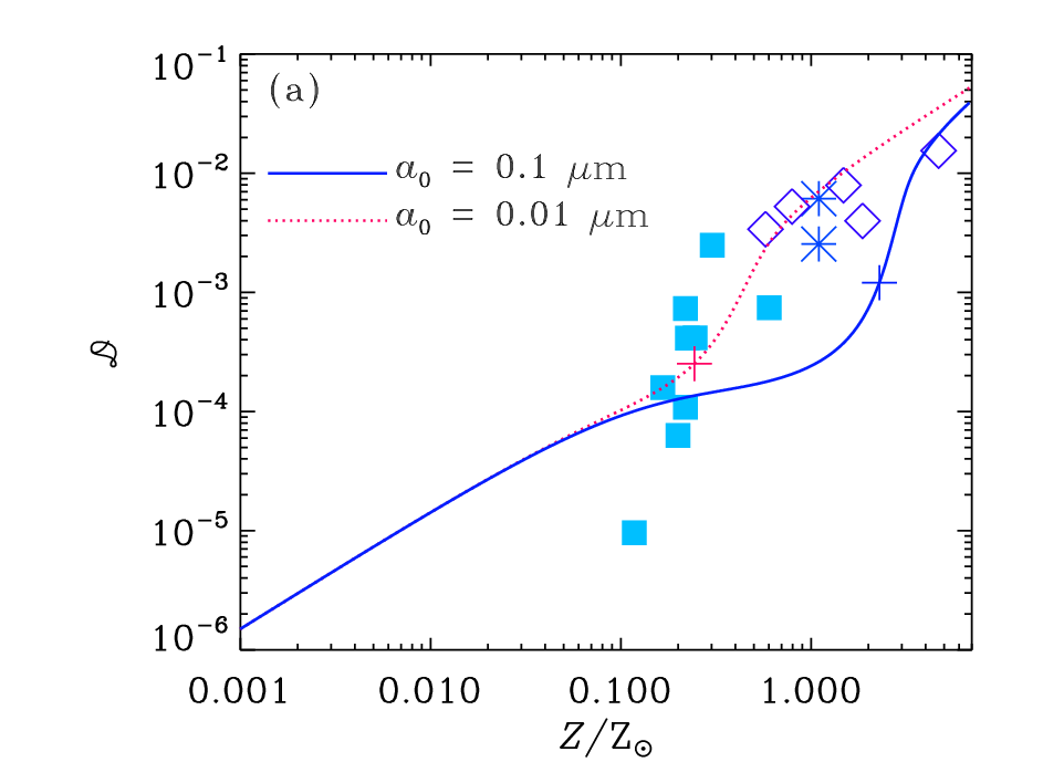
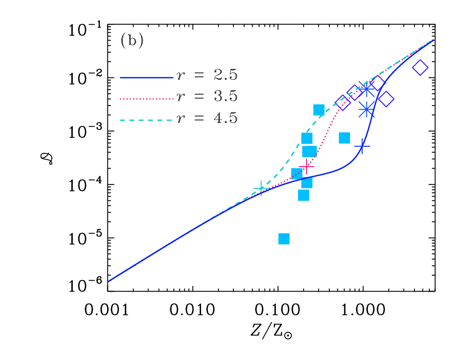
The relations between dust-to-gas ratio and metallicity are shown in Fig. 8 for $f_{\mathrm{in}}=0.1$ and in Fig. 9 for $f_{\mathrm{in}}=0.01$. We assume Z${}_{☉}=0.015$ (Lodders, 2003). At low metallicity levels, the solution of equation (54) is approximated by $\mathcal{D}\sim f_{\mathrm{in}}Z$. This is why the dust-to-gas ratio in the low-metallicity regime is lower in Fig. 9 than in Fig. 8. Above a certain metallicity level, a rapid increase of dust-to-gas ratio occurs because of the grain growth in clouds. The metallicity level at which this growth occurs is very sensitive to the grain size distribution.

The observational data of nearby galaxies are also shown for comparison. For the uniformity of data, we select the samples observed by AKARI: blue compact dwarf galaxies in Hirashita & Ichikawa (2009) and spiral galaxies (M 81 from Sun & Hirashita 2011 and M 101 from Suzuki et al. 2007). The dust masses are estimated from 90 $\micron$ and 140 $\micron$ data by using the mass absorption coefficient in Hirashita & Ichikawa (2009). For the gas mass of the dwarf galaxies and M 81, we adopt the H i mass, since the molecular mass is negligible or not detected. The H i masses of M 81 and of the dwarf galaxies are taken from Walter et al. (2008) and in Hirashita & Ichikawa (2009), respectively. For M 101, we adopt the sum of neutral and molecular gas masses compiled in Suzuki et al. (2007). The oxygen abundance is adopted for the indicator of the metallicity, and the solar abundance is assumed to be $12+\log\mathrm{(O/H)}=8.69$ (Lodders, 2003). The oxygen abundances of the dwarf galaxies are compiled in Hirashita & Ichikawa (2009), and those of the spiral galaxies at the half-light radius are taken from Garnett (2002). Typical errors of the observational quantities are comparable to the size of symbols in the figures. To ensure that the AKARI results are not systematically different from other results, we add the data in Issa, MacLaren, & Wolfendale (1990), who estimated the dust mass from the extinction. The overall trend of the data is reproduced by the models.

Asano et al. (2011) also include a sample whose dust mass is derived from Spitzer observations by Engelbracht et al. (2008) and show that the relation between dust-to-gas ratio and metallicity does not significantly change. The inclusion of Herschel data may boost the dust abundance because of the possible contribution from very cold dust especially in dwarf galaxies (Grossi et al., 2010). Galliano et al. (2005) also find a large contribution from very cold dust in the submillimetre for some dwarf galaxies. However, since the modeling of submillimetre emission may be significantly affected by the assumed emissivity index of large grains, we do not use the submillimetre data in this paper. We should keep in mind that that inclusion of submillimetre data can rather decrease the dust mass especially for dust-rich galaxies because the dust temperature estimate becomes better (Galametz et al., 2011). In their models, the Spitzer 160 $\micron$ data are used; thus, it is not still unclear if there is a discrepancy between the dust temperatures estimated by AKARI and those estimated by including submillimetre data. The dust mass in M 81 derived by the Herschel observation ($3.4\times 10^{7}$ M_⊙; Bendo et al. 2010) is similar to that estimated by the AKARI observation adopted in this paper ($3.2\times 10^{7}$ M_⊙; Sun & Hirashita 2011).

We have shown that the grain size distribution significantly affects the evolution of dust mass above a certain metallicity level where the grain growth in clouds is activated. In fact, as shown in Figs. 8 and 9, the difference in the grain size distribution makes a significant imprint in the relation between dust-to-gas ratio and metallicity. This comes from the dependence of $\beta$ on metallicity. As shown in equation (37), $\beta\propto(\tau_{\mathrm{grow}}/\tau_{\mathrm{cl}})^{-1}$. Fig. 6 shows that $\tau_{\mathrm{grow}}/\tau_{\mathrm{cl}}$ is a decreasing function of metallicity. Thus, $\beta$ increases as the system is enriched with metals, and if the last term in equation (54) becomes positive at a certain metallicity, the dust mass grows in a nonlinear way. Because $\beta$ (or $\tau_{\mathrm{grow}}/\tau_{\mathrm{cl}}$) is sensitive to the grain size distribution, the resulting relation between dust-to-gas ratio and metallicity depends largely on the grin size distribution. In other words, the metallicity level at which the grain growth in clouds is activated varies sensitively with the grain size distribution. This metallicity level is called ‘critical metallicity’, which is quantified and discussed in the next subsection.

Asano et al. (2011) and Inoue (2011) have shown that the grain growth by accretion dominates the grain abundance if the metallicity is larger than a certain ‘critical metallicity’. As mentioned in the previous subsection, the nonlinear increase of dust-to-gas ratio by grain growth is realized when $-\beta_{\mathrm{SN}}-\mathcal{R}+\beta/\epsilon>0$ in equation (54). Since $\beta_{\mathrm{SN}}\gg\mathcal{R}$, the critical metallicity, $Z_{\mathrm{cr}}$, can be estimated by the metallicity at which $\beta$ as a function of metallicity realizes

where $\beta(Z)$ indicates that $\beta$ is a function of metallicity. In our models, $\epsilon=0.1$ and $\beta_{\mathrm{SN}}=9.65$, i.e., $\beta(Z_{\mathrm{cr}})=0.965$. Therefore, if the metallicity is so high that the grain growth in individual clouds increases the dust mass by 0.965 times the original dust amount, the grain growth becomes prominent. The critical metallicity varies by a factor of $\sim 1.5$ if we change $\beta_{\mathrm{SN}}$ by a factor of 2 (i.e. uncertainty in $\beta_{\mathrm{SN}}$ from the assumed species; Jones & Nuth 2011).

The position for the critical metallicity is marked on each line in Figs. 8 and 9 and listed in Table 3 (for $f_{\mathrm{in}}=0.1$ but $Z_{\mathrm{cr}}$ only decrease by $\sim 10$–20 per cent for $f_{\mathrm{in}}=0.01$). Indeed the dust-to-gas ratio rapidly increases if the metallicity becomes larger than the critical metallicity. This supports Inoue (2011)’s view that the activation of grain growth is driven by the metallicity. In this paper we have found that the critical metallicity is sensitive to the grain size distribution. If the major part of the grains are as large as $\sim 0.1~\micron$, the grain growth is activated above $\sim 2$ Z_☉, which is too large to explain the large grain abundance in the objects with sub-solar metallicities. If the typical grain size is as small as $\sim 0.01~\micron$ or the grain size distribution is described by a power law with $r\ga 3.5$, the large grain abundance in sub-solar metallicity galaxies can be naturally explained by the efficient grain growth in clouds. Therefore, the evolutionary history of grain size distribution is important to understand the grain abundance in galaxies.

By an analysis of infrared dust emission spectra, Galliano et al. (2005) show that the grain size distributions of some metal-poor dwarf galaxies are biased toward smaller grains compared with the Galactic case (i.e. $r\simeq 3.5$). Therefore, the critical metallicity for these dwarf galaxies is expected to be lower than their metallicities: in other words, the grain growth in clouds is expected to contribute significantly to the dust abundance in these galaxies. It is interesting to point out that $r=4.5$ explains the data points of metal-poor galaxies better than $r=3.5$. This is consistent with Galliano et al. (2005)’s conclusion that the grain size distribution is biased to small sizes.

After the grain growth, all the lines in Figs. 8 and 9 finally converge. This is explained as follows. If the metallicity is high enough, the grain growth is regulated by the lifetime of clouds and is independent of grain size distribution. In other words, $\beta\sim\xi/(1-\xi)$ if the metallicity becomes high enough (i.e. $y$ is large enough in equation 42). Using $\xi=1-\mathcal{D}/Z$ and equation (54), we obtain the following estimate in the case where the grain growth dominates the increase of the dust content:

which is valid for $Z>Z_{\mathrm{c}}$ (we only adopt the dominant terms). Therefore, if $\xi$ is so small (large) that the right-hand side of this equation is positive (negative), $\xi$ tends to increase (decrease) as $Z$ increases. This means that $\xi$ tends to approach the value that makes the right-hand side to be zero; that is,

For the values adopted in our models ($\epsilon=0.1$ and $\beta_{\mathrm{SN}}=9.65$), $\xi\sim 0.49$. This means that the fraction of metals in dust phase is about 0.5 at metallicities much higher than the critical metallicity. If we consider the uncertainty in $\beta_{\mathrm{SN}}$ by a factor of 2 because of material difference (Jones & Nuth, 2011), $\xi\sim 0.33$–0.66.

It is interesting that $\xi$ at $Z\gg Z_{\mathrm{cr}}$ only depends on $\epsilon\beta_{\mathrm{SN}}$. Using the definition of $\beta_{\mathrm{SN}}=\epsilon_{\mathrm{s}}M_{\mathrm{s}}\gamma/\psi$ (below equation 50) and equation (43), we obtain

This is the ratio between the gas mass swept by SN shocks per unit time multiplied by the efficiency of dust destruction in SN shocks, and the formation rate of clouds. In other words, this is the ratio between the dust destruction rate by SN shocks and the grain growth rate in clouds. Therefore, it is natural that the final fraction of metals in dust phase can be described by the balance between the dust destruction by SN shocks and the dust formation in clouds.

Inoue (2011) also obtained a similar expression for the critical metallicity. We have confirmed his conclusion that the dust-to-metal ratio approaches a constant value: this behaviour is called self-regulation by Inoue (2011). The difference between our formulation and his is that he treated $\tau_{\mathrm{SF}}$ as a parameter independent of $\tau_{\mathrm{grow}}$ while we connect these two parameters through the star formation efficiency $\epsilon$. Since both star formation and grain growth occur in molecular clouds, these two processes are not independent. Moreover, if the grain growth is efficient enough, the dust growth time-scale is limited by the lifetime of clouds, which is independent of the grain size distribution. Therefore, the dust-to-metal ratio does not depend on the grain size distribution for $Z\gg Z_{\mathrm{cr}}$, and it depends only on $\epsilon\beta_{\mathrm{SN}}$.

The first dust should be produced by SNe in the death of massive stars. Because of shock destruction in SNe, the dust sizes may be biased to $a\ga 0.1~\micron$ (Bianchi & Schneider, 2007; Nozawa et al., 2007). Hirashita et al. (2010) show that shattering driven by interstellar turbulence can produce small grains efficiently if the metallicity becomes higher than a critical value ($\sim 0.1$–1 Z_☉). Thus, the critical metallicity for the grain growth is near the metallicity level where shattering produces small grains efficiently. The production of small grains accelerates the grain growth by accretion, which raises the grain abundance. With the increased dust abundance, shattering can be further efficient, although the produced small grains by shattering does not necessarily activate further shattering of large grains (Jones et al., 1996). Such an interplay between shattering and accretion may be interesting to investigate in the future.

The size distribution of grains produced by AGB stars is also important since AGB stars become the dominant dust production source after several hundreds of Myr (Valiante et al., 2009; Gall et al., 2011a; Asano et al., 2011). The size of grains produced in AGB stars is suggested to be large ($a\sim 0.1~\micron$) from the observations of spectral energy distributions (Groenewegen, 1997; Gauger et al., 1999), although Hofmann et al. (2001) show that the grains are not single-sized. To clarify the grain size distribution formed by AGB stars is important for the efficiency of grain growth. Shattering in the ISM may also play a role in efficiently producing small grains even if AGB stars only produce large grains (Hirashita, 2010). In this case, efficient grain growth can occur.

It is interesting to point out that the critical metallicity is within the metallicity range typical of dwarf galaxies (Table 3). This confirms the conclusion by Asano et al. (2011) that the strong metallicity dependence of the dust-to-gas ratio in dwarf galaxies can be explained by the grain growth in clouds.

The grain growth is also important in some high-redshift galaxy populations. In fact, high-redshift quasars have solar (or more) metallicities (Juarez et al., 2009, e.g.), which implies that the grain growth is indeed governing the dust abundance in distant quasars (Michałowski et al., 2010; Pipino et al., 2011; Asano et al., 2011) (Valiante et al., 2009; Gall et al., 2011b, but see). If the abundance of small grains are enhanced because of shattering as suggested by Hirashita et al. (2010), the critical metallicity becomes lower, so that the importance of grain growth in clouds is further pronounced.

Qualitatively it may be predicted that the mid-infrared emission from very small grains is relatively suppressed if the grain growth in clouds is activated. However, it is hard to quantitatively predict the galaxy-scale observational features caused by the grain growth in clouds because it is difficult to selectively see the clouds, where grain growth is occurring. Since observations of galactic spectral energy distribution inevitably include the emission from diffuse medium, other mechanisms modifying the grain size distribution such as shattering and coagulation are also reflected in the observed emission from grains. Indeed, Galliano et al. (2005) show that the grain size distribution is biased toward smaller grains in some dwarf galaxies, which may be interpreted as the efficient grain processing in diffuse medium. They also demonstrate that there is a variety in the grain size distribution among dwarf galaxies. Such a variety will be investigated in the future with a consistent treatment of a nonlinear combination between the small grain production by shattering and sputtering and the grain growth by accretion and coagulation.

References

- Asano et al. (2011) Asano, R. S., Takeuchi, T. T., Hirashita, H., & Inoue, A. K. 2011, A&A, submitted
- Bendo et al. (2010) Bendo, G. J., et al. 2010, A&A, 518, L65
- Bianchi & Schneider (2007) Bianchi, S., & Schneider, R. 2007, MNRAS, 378, 973
- Calura et al. (2008) Calura, F., Pipino, A., & Matteucci, F. 2008, A&A, 479, 669
- Compiègne et al. (2011) Compiègne, M. et al. 2011, A&A, 525, A103
- Désert, Boulanger, & Puget (1990) Désert, F.-X., Boulanger, F., & Puget, J. L. 1990, A&A, 237, 215
- Draine (2009) Draine, B. T. 2009, in Henning Th., Grün E., Steinacker J., eds, Cosmic Dust – Near and Far. ASP Conf. Ser., ASP, San Francisco, p. 453
- Draine & Lee (1984) Draine, B. T., & Lee, H. M. 1984, ApJ, 285, 89
- Dwek (1998) Dwek, E. 1998, ApJ, 501, 643
- Engelbracht et al. (2008) Engelbracht, C. W., Rieke, G. H., Gordon, K. D., Smith, J.-D. T., Werner, M. W., Moustakas, J., Willmer, C. N. A., & Vanzi, L. 2008, ApJ, 678, 804
- Evans (1994) Evans, A. 1994, The Dusty Universe, Wiley, Chichester
- Fukui & Kawamura (2010) Fukui, Y., & Kawamura, A. 2010, ARA&A, 48, 547
- Galametz et al. (2011) Galametz, M., Madden, S. C., Galliano, F., Bendo, G. J., & Sauvage, M. 2011, A&A, in press
- Gall et al. (2011a) Gall, C., Andersen, A. C., & Hjorth, J. 2011a, A&A, 528, A13
- Gall et al. (2011b) Gall, C., Andersen, A. C., & Hjorth, J. 2011b, A&A, 528, A14
- Galliano et al. (2005) Galliano, F., Madden, S. C., Jones, A. P., Wilson, C. D., & Bernard, J.-P. 2005, A&A, 434, 867
- Galliano et al. (2003) Galliano, F., Madden, S. C., Jones, A. P., Wilson, C. D., Bernard, J.-P., & Le Peintre, F. 2003, A&A, 407, 159
- Garnett (2002) Garnett, D. R. 2002, ApJ, 581, 1019
- Gauger et al. (1999) Gauger, A., Balega, Y. Y., Irrgang, P., Osterbart, R., & Weigelt, G. 1999, A&A, 346, 505
- Gavazzi et al. (2002) Gavazzi, G., Bonfanti, C., Sanvito, G., Boselli, A., & Scodeggio, M. 2002, ApJ, 576, 135
- Grassi et al. (2011) Grassi, T., Krstic, P., Merlin, E., Buonomo, U., Piovan, L., & Chiosi, C. 2011, A&A, in press
- Groenewegen (1997) Groenewegen, M. A. T. 1997, A&A, 317, 503
- Grossi et al. (2010) Grossi, M., et al. 2010, A&A, 518, L52
- Guillet et al. (2007) Guillet, V., Pineau des Forêts, G., & Jones, A. P. 2007, A&A, 476, 263
- Guillet et al. (2011) Guillet, V., Pineau des Forêts, G., & Jones, A. P. 2011, A&A, 527, A123
- Hirashita (2000a) Hirashita, H. 2000a, PASJ, 52, 585
- Hirashita (2000b) Hirashita, H. 2000b, ApJ, 531, 693
- Hirashita (2010) Hirashita, H. 2010, MNRAS, 407, L49
- Hirashita & Ichikawa (2009) Hirashita, H., & Ichikawa, T. T. 2009, MNRAS, 396, 500
- Hirashita et al. (2010) Hirashita, H., Nozawa, T., Yan, H., & Kozasa, T. 2010, MNRAS, 404, 1437
- Hirashita & Yan (2009) Hirashita, H., & Yan, H. 2009, MNRAS, 394, 1061
- Hofmann et al. (2001) Hofmann, K.-H., Balega, Y., Blöcker, T., & Weigelt, G. 2001, A&A, 379, 529
- Inoue (2003) Inoue, A. K. 2003, PASJ, 55, 901
- Inoue (2011) Inoue, A. K. 2011, Earth, Planets, and Space, submitted
- Issa et al. (1990) Issa, M. R., MacLaren, I., & Wolfendale, A. W. 1990, A&A, 236, 237
- Jones & Nuth (2011) Jones, A. P., & Nuth, J. A., III 2011, A&A, submitted
- Jones et al. (1996) Jones, A. P., Tielens, A. G. G. M., & Hollenbach, D. J. 1996, ApJ, 469, 740
- Jones et al. (1994) Jones, A., Tielens, A. G. G. M., Hollenbach, D. J., McKee, C. F. 1994, ApJ, 433, 797
- Juarez et al. (2009) Juarez, Y., Maiolino, R., Mujica, R., Pedani, M., Marinoni, S., Nagao, T., Marconi, A., & Oliva, E. 2009, A&A, 494, L25
- Kennicutt (1998) Kennicutt, R. C., Jr. 1998, ARA&A, 36, 189
- Kozasa et al. (2009) Kozasa, T., Nozawa, T., Tominaga, N., Umeda, H., Maeda, K., & Nomoto, K. 2009, in Henning Th., Grün E., Steinacker J., eds, Cosmic Dust – Near and Far. ASP Conf. Ser., ASP, San Francisco, p. 43
- Lada, Lombardi, & Alves (2010) Lada, C. J., Lombardi, M., & Alves, J. F. 2010, ApJ, 724, 687
- Leisawitz, Bash, & Thaddeus (1989) Leisawitz, D., Bash, F. N., & Thaddeus, P. 1989, ApJS, 70, 731
- Leitch-Devlin & Williams (1985) Leitch-Devlin, M. A., & Williams, D. A. 1985, MNRAS, 213, 295
- Lisenfeld & Ferrara (1998) Lisenfeld, U., & Ferrara, A. 1998, ApJ, 496, 145
- Lodders (2003) Lodders, K. 2003, ApJ, 591, 1220
- Mathis, Rumpl, & Nordsieck (1977) Mathis, J. S., Rumpl, W., & Nordsieck, K. H. 1977, ApJ, 217, 425 (MRN)
- McKee (1989) McKee, C. F. 1989, in Allamandola L. J. & Tielens A. G. G. M. eds., IAU Sump. 135, Interstellar Dust, Kluwer, Dordrecht, 431
- Michałowski et al. (2010) Michałowski, M. J., Murphy, E. J., Hjorth, J., Watson, D., Gall, C., & Dunlop, J. S. 2010, A&A, 522, A15
- Nozawa et al. (2007) Nozawa, T., Kozasa, T., Habe, A., Dwek, E., Umeda, H., Tominaga, N., Maeda, K., & Nomoto, K. 2007, ApJ, 666, 955
- O’Donnell & Mathis (1997) O’Donnell, J. E., & Mathis, J. S. 1997, ApJ, 479, 806
- Ormel et al. (2009) Ormel, C. W., Paszun, D., Dominik, C., & Tielens, A. G. G. M. 2009, A&A, 502, 845
- Pipino et al. (2011) Pipino, A., Fan, X. L., Matteucci, F, Calura, F., Silva, L., Granato, G., & Maiolino, R. 2011, A&A, 525, A61
- Savage & Sembach (1996) Savage, B. D., & Sembach, K. R. 1996, ARA&A, 34, 279
- Serra Díaz-Cano & Jones (2008) Serra Díaz-Cano, L., & Jones, A. P. 2008, A&A, 492, 127
- Sun & Hirashita (2011) Sun, A.-L., & Hirashita, H. 2011, MNRAS, 411, 1070
- Suzuki et al. (2007) Suzuki, T., Kaneda, H., Nakagawa, T., Makiuti, S., & Okada, Y. 2007, PASJ, 59, 473
- Valiante et al. (2009) Valiante, R., Schneider, R., Bianchi, S., & Andersen, A. C. 2009, MNRAS, 397, 1661
- Walter et al. (2008) Walter, F., Brinks, E., de Blok, W. J. G., Bigiel, F., Kennicutt, R. C., Thornley, M. D., & Leroy, A. 2008, AJ, 136, 2563
- Weingartner & Draine (1999) Weingartner, J. C., & Draine, B. T. 1999, ApJ, 517, 292
- Weingartner & Draine (2001) Weingartner, J. C., & Draine, B. T. 2001, ApJ, 548, 296
- Yamasawa et al. (2011) Yamasawa, D., Habe, A., Kozasa, T., Nozawa, T., & Hirashita, H. 2011, ApJ, in press
- Yan et al. (2004) Yan, H., Lazarian, A., & Draine, B. T. 2004, ApJ, 616, 895
- Zhukovska et al. (2008) Zhukovska, S., Gail, H.-P., & Trieloff, M. 2008, A&A, 479, 453
Appendix A Instantaneous recycling approximation
We estimate and used in Section 4.4. With an initial mass function (IMF) , and are written as