Symmetry and Topology in Superconductors
- Odd-frequency pairing and edge states -
Abstract
Superconductivity is a phenomenon where the macroscopic quantum coherence appears due to the pairing of electrons. This offers a fascinating arena to study the physics of symmetry breaking, i.e., broken gauge symmetry. However, the important symmetries in superconductors are not only the gauge invariance. Especially, the symmetry properties of the pairing, i.e., the parity and spin-singlet / spin-triplet, determine the physical properties of the superconducting state. Recently it has been recognized that there is the important third symmetry of the pair amplitude, i.e., even or odd parity with respect to the frequency. The conventional uniform superconducting states correspond to the even-frequency pairing, but the recent finding is that the odd-frequency pair amplitude arises in the spatially non-uniform situation quite ubiquitously. Especially, this is the case in the Andreev bound state (ABS) appearing at the surface/interface of the sample. The other important recent development is on the nontrivial topological aspects of superconductors. As the band insulators are classified by topological indices into (i) conventional insulator, (ii) quantum Hall insulator, and (iii) topological insulator, also are the gapped superconductors. The influence of the nontrivial topology of the bulk states appears as the edge or surface of the sample, i.e., bulk-edge correspondence. In the superconductors, this leads to the formation of zero energy ABS (ZEABS). Therefore, the ABSs at the surface/interface of the superconductors are the place where the symmetry and topology meet each other which offer the stage of rich physics. In this review, we discuss the physics of ABS from the viewpoint of the odd-frequency pairing, the topological bulk-edge correspondence, and the interplay of these two issues. It is described how the symmetry of the pairing and topological indices determine the absence/presence of the ZEABS, its energy dispersion, and properties as the Majorana fermions. Various related issues such as the Helium 3, transport of Majorana fermions, and tunneling spectroscopies are also briefly discussed.
Keywords:
Odd-frequency pairing, Andreev bound state, Bulk-edge correspondence, Majorana fermion, Topological index1 Introduction
Two of the most important principles in physics are symmetry and topology, both of which are related to the quantum numbers and energy degeneracy of states [1]. For the compact symmetry group such as the rotation, the discrete quantum numbers result. However, even a slight breaking of the symmetry destroys these features, i.e., the conservation law is violated and the degeneracy is lifted. In the many-body systems, it often happens that the symmetry is spontaneously broken as a collective phenomenon. Ferromagnetism and superconductivity are two representative examples of this spontaneous symmetry breaking characterized by the order parameters. The magnetization, which breaks the rotational symmetry in the spin space, and the pair amplitude, which breaks the gauge symmetry, are the corresponding order parameters, respectively. In sharp contrast to this, the topological quantum numbers are more robust against the perturbations. For example, the quantization of the magnetic flux captured by one vortex in a superconductor is quantized to be even in the disordered case without the cylindrical symmetry. This is guaranteed by the single-valued property of the superconducting order parameter and the stability of its winding number. It is evident that the winding number around a singular point ( the center of the vortex in the above example) does not change for the continuous deformation as long as the path does not cross the singular point. Therefore, the topological properties often lead to the robustness of the system against the weak and moderate perturbations protected by the topological quantum number.
It is not always clear how to separate the two origins of the quantum numbers, i.e., symmetry and topology. Even more interesting is the interplay between these two principles. It often happens that they are entangled to give a rich variety of physical phenomena. In this review article, we describe how these two principles are merged into the novel properties of superconductors.
1.1 Symmetry classifications of bulk superconductors and relevant quantum phenomena
Symmetry of Cooper pair is a central topic in the physics of superconductivity. Here we discuss uniform bulk systems. It is established that Cooper pair is formed between two electrons. In accordance with the Fermi-Dirac statistics, pair amplitude, which is a wave function of Cooper pair, must have a sign change with the exchange of two electrons. Symmetry of Cooper pair is customary classified into spin-singlet even-parity and spin-triplet odd-parity where even (odd) refers to the orbital part of the pair amplitude. For example, -wave and -wave pairings belong to the former case while -wave pairing belongs to the latter [2]. With broken inversion symmetry, spatial parity is no more a good quantum number. In that case, spin-singlet even-parity and spin-triplet odd-parity pairings can mix with each other. The mixed parity pairing has become an important issue in non-centrosymmetric superconductors [3, 4]. It is noted that both in spin-singlet even-parity and spin-triplet odd-parity pairings, the pair amplitude does not have a sign change with the exchange of two time variables for the two electrons forming the Cooper pair. However, there is a possibility that pair amplitude has a sign change by this operation [5]. The latter type of pairing is so called odd-frequency pairing originally proposed by Berezinskii [6]. There are two possibilities of odd-frequency pairing, , spin-singlet odd-parity and spin-triplet even-parity pairings. Thus, in the presence of both the inversion and spin-rotational symmetries, Cooper pairs are classified into (i)even-frequency spin-singlet even-parity (ESE), (ii)even-frequency spin-triplet odd-parity (ETO), (iii)odd-frequency spin-triplet even-parity (OTE), and (iv)odd-frequency spin-singlet odd-parity (OSO). In strongly correlated systems, due to the retardation effect of the electron interaction, there is a possibility for odd-frequency pairing in the bulk. After the prediction by Berezinskii[6], there have been several theoretical proposals about odd-frequency pairing in the bulk [7, 8, 9, 10, 11, 12, 13, 14, 15, 16, 17]. However, up to now, odd-frequency bulk superconductor has not been established experimentally yet. Although it is not easy to realize odd-frequency gap function in uniform bulk systems, it is more promising to induce odd-frequency pair amplitude in the non-uniform system with lower symmetry.
| Class | Time | Spin | Orbital | Total |
| ESE | + | + | ||
| ETO | + | + | ||
| OTE | + | + | ||
| OSO |
Bergeret, Volkov and Efetov have clarified that in ferromagnet/superconductor heterostructures with inhomogeneous magnetization, odd-frequency pairing is generated in ferromagnet [18]. They have predicted the long range proximity effect by the odd-frequency pairing. Furthermore, one of the authors (Y.T.) has revealed that the odd-frequency pairing is possible in inhomogeneous superconducting systems even without magnetic ordering [19, 20, 21]. We will show ubiquitous presence of odd-frequency pairing in §2 [20, 22].
Symmetry of the Cooper pair influences tunneling phenomena in superconducting heterostructures. It is known that Andreev bound state (ABS) is generally generated at the surface of anisotropic superconductor where pair potential (energy gap function) has a sign change on the Fermi surface [23, 24, 25, 26, 27, 28, 29, 30, 31]. By properly taking into account of the Andreev reflection in anisotropic superconductors [32, 33, 34], it has been proven that the ABS manifests itself as a zero bias conductance peak (ZBCP) of quasiparticle tunneling spectroscopy [28, 25, 35]. The presence of ZBCP has been observed in tunneling spectroscopy of high cuprates [36, 37, 38, 39, 40, 41, 42, 43]. It has been established that a dispersionless zero energy ABS (ZEABS) [25] is generated at the surface for spin-singlet -wave superconductors. The existence of the ABS influences seriously on charge transport [44, 45, 46], spin transport [47] and magnetic responses [48, 49, 50].
ABS is also expected for spin-triplet -wave superconductors. It induces ZBCP in the tunneling spectroscopy [51, 52]. However, proximity effect via ABS is completely different between spin-singlet superconductors and spin-triplet superconductors. The ABS cannot penetrate into a diffusive normal metal (DN) attached to the superconductor in the former case, while it is possible in the latter one. The underlying physics can be expressed by the symmetry of the induced odd-frequency pairing [19]. We will discuss these exotic phenomena in §2.
1.2 Topological orders and topological quantum numbers
Up to now, we have discussed the classifications of the superconductors by symmetry as an example of quantum states. Then, is there any other way to characterize the quantum phases of electronic systems ? The answer is yes, and the topological orders and topological quantum numbers serve this purpose [53]. Historically, the first topological ordered state in condensed matter physics is the quantum Hall system, , the two-dimensional electronic systems under strong magnetic field at low temperature, where the Hall conductance is quantized to be the integer times the unit (integer quantum Hall effect (IQHE)) or its fractions (fractional quantum Hall effect (FQHE)) (: unit charge, : Planck constant). Here, the topological quantum number (integer, see eq.(54)) characterizing the topological order is related to the physical observable, i.e., the Hall conductance as
| (1) |
which explains why is quantized as the integer multiple of [54].
Another important issue related to the IQHE is the one-dimensional channels along the edge of the sample [55]. A classical picture for these edge channels is that the cyclotron motion of the electrons in the bulk is reflected at the boundary of the sample, forming the one-dimensional motion in one-direction. This property of ”one-direction” is called ”chiral”. In the quantum mechanical picture, the two-dimensional electronic states under magnetic field form the Landau levels, whose energies are pushed up near the edges of the sample by the confining potential. As a consequence, some of the edge channels cross the Fermi energy, which carry current. A remarkable fact is that the direction of the propagating waves along these edge channels is one-way, i.e., chiral, and those with the opposite direction are on the other side of the sample, i.e., far away separated by the bulk. (Consider the cylindrical sample where the two edges are separated by the bulk.) Therefore, the backward scattering is strictly forbidden even if the impurity potential is there. This leads to the perfect one-dimensional conductance of each channel, and consequently the Hall conductance is given by
| (2) |
where is the number of the edge channels including the sign representing the chirality. Comparing eqs.(1) and (2), one concludes that there is a relation between the bulk topological quantum number () and the edge channels () [56, 57]. This is called ”bulk-edge correspondence” and will be explored more in details later. One can say that the one-dimensional electronic states are ”split into halves” at the two edges of the sample according to the chiralities, and the fractionalized electrons become robust. This fractionalization of the electrons at the edge is realized/supported by the topological order in the bulk state.
FQHE is a more complex phenomenon where the electron-electron interaction plays the essential role. Therefore, one needs to study the many-body wave functions, and the topological quantum numbers characterizing the quantum states are much more intriguing. The readers are referred to the textbooks for the details [1, 53]. However, conceptually the story is quite analogous and similar to the IQHE. The topological order in the bulk reflects itself as the edge channels at the boundary of the sample, i.e., the bulk-edge correspondence occurs.
A recent breakthrough is the discovery of the topological insulators which preserve the time-reversal symmetry , i.e., without the external magnetic field or the spontaneous magnetization [58, 59]. With -symmetry, the Hall response and hence the Chern number is zero. Therefore, it is required to define new topological quantum numbers to characterize the topological orders.
The concept of topologically nontrivial states of the single-particle Hamiltonian can be generalized to the superconducting state as long as one considers the BCS Hamiltonian in the Nambu representation;
| (3) |
where A naive way is to consider the matrix elements of as that of the Bloch states discussed above. However, the situation is not so trivial since the degrees of freedom are redundant in and . Consequently, the edge channels and surface states originating from the bulk-edge correspondence has the same redundancy, which sometimes leads to Majorana fermion. The present edge channels and surface states appear as the ABSs characterized by the symmetry of Cooper pair as discussed in the former subsection. Therefore, the physics is much richer in this topological superconductor than the non-interacting electron systems.
In this review, we discuss the recent developments on the topological superconductors as the merging point of the two principles, i.e., symmetry and topology. The in-depth study of this issue will clarify the interplay between these two principles in physics. The plan of this review follows. In §2, the odd-frequency superconducting pairing induced by the extrinsic symmetry breaking such as spatial non-uniformity and/or the time-reversal symmetry breaking is studied to demonstrate how the superconductivity is influenced by the symmetries. In §3, we discuss the topology of the bulk states in superconductors and its relation to the surface/edge states (bulk-edge correspondence). Various related issues are described in §4. §4 is also devoted to the summary and future perspectives. Hereafter, we choose the unit unless explicitly written. Two key concepts in this review are odd-frequency pairing and edge states. In Fig.1, we show the relations between each subsection and above two key concepts explicitly. The readers who want to know the essence of the review urgently would be appreciated to look at Table IX in §4.

2 Extrinsic symmetry breaking and odd-frequency pairing in superconductors
2.1 What is extrinsic symmetry breaking ?
In this section, we discuss what is an extrinsic symmetry breaking. Typical examples are breaking of the translational invariance or that of spin-rotational symmetry. In general, Cooper pair is formed between position and . Pair amplitude is a function of and . When we focus on the symmetry with respect to the exchange of two coordinates and , i.e., , we can define the parity of the Cooper pair. We employ the Fourier transformation from to . If we consider inhomogeneous superconducting systems, like vortex and junctions, translational symmetry is broken. In that system, parity of the Cooper pair is no more a good quantum number. Then, near the vortex core or the interface / surface of the superconductor, mixed parity state can be realized. To be more specific, let us consider normal metal / superconductor (N/S) junction where the symmetry of the superconductor belongs to ESE. Near the interface or in the normal metal, due to the breaking of translational symmetry, odd-parity state can be mixed. Since the spin rotational symmetry is not broken, pairing symmetry of spin should be singlet. To be consistent with Fermi Dirac statistics, the resulting Cooper pair should be odd in frequency. Then, we can expect OSO paring is generated [19] near the interface and also inside normal metal. On the other hand, if symmetry in the bulk is ETO, then the induced pairing symmetry by breaking of the translational invariance or the spatial inversion symmetry is OTE.
Next, we discuss the breaking of the spin rotational symmetry only. By this symmetry breaking, spin-singlet and spin-triplet parings are mixed with each other. Let us consider superconductor with ESE symmetry. In the presence of Zeeman magnetic field, spin-triplet pairing state is generated. Since spatial parity is not broken, the induced pair amplitude should be OTE. On the other hand, if the pairing in the bulk is ETO, then the induced pair amplitude by breaking of spin rotational symmetry is OSO.
From this viewpoint, paring symmetry in ferromagnet / superconductor (F/S) junction is very interesting. Here, we specify that the symmetry of the superconductor is spin-singlet -wave one which belongs to ESE. In the light of above discussion, OSO pairing is induced in F by translational symmetry breaking. Also by the spin rotational symmetry breaking, OTE (ETO) pairing is generated from ESE (OSO) pairing. Thus, in F, all four kinds of pairings are basically possible [22]. In the standard case accessible in experiments, F is in the diffusive regime. Then, basically only -wave pairing is possible since it is robust against impurity scattering [60]. The resulting paring symmetries in F are only ESE -wave and OTE -wave. It has been shown that OTE pairing seriously influences on the density of states of quasiparticles. When OTE -wave pairing dominates, quasiparticle density of state does not have a gap-like structure around zero energy[61]. In the extreme case, it has a zero energy peak (ZEP) structure [61, 62].
2.2 N/S junction with ballistic system
In this subsection, we consider superconducting proximity effect and resulting ubiquitous presence of odd-frequency pairing in N / S junctions [63]. In general, physical quantities have spatial dependence near the interface. There are two characteristic length scales: i) The inverse of the Fermi wave length and ii) coherence length given by , where is the Fermi velocity and is the energy gap (pair potential) in the superconductor. Here, we are interested in physical quantities varying slowly over the coherence length. In the present situation, it is appropriate to use quasiclassical Green’s function method where high energy degrees of freedom are integrated out[64, 65, 66, 67]. The quasiclassical Green’s function is obtained from Gor’kov Green’s function by integrating the energy and is concentrating on the low energy scale measured from the Fermi energy level. In this approximation, quasiparticles feel the pair potential depending on their direction of their motions on the Fermi surface.
In the following, we consider two-dimensional N () / S () junctions in the ballistic limit (Fig. 2). For the bulk superconductor, we choose even-frequency ESE or ETO pairings. As regards the spin-triplet ETO pairing, we choose for simplicity. There is no essential difference even if we consider spin-triplet pairing with . We assume a thin insulating barrier located at the N/S interface () modeled by a delta functional potential . The reflection coefficient and transmission coefficient of the junction for the quasiparticle with the injection angle is given by and , respectively, with , where is measured from the normal to the interface.

Here, we introduce quasiclassical retarded (advanced) Green’s functions , and where is given by . () is the Green’s function of quasiparticle at position , energy with injection angle (). denotes anomalous Green’s function which becomes zero in the normal state. can be decomposed into and ,
with
| (4) |
From this definition, it is clear that () corresponds to the odd (even)-frequency pairing. Due to the translational invariance in the direction parallel to the interface , we can simply replace by . , , and satisfy following so called the Eilenberger equation [68]
| (5) |
with
and
Here, () is the Pauli matrix in the electron-hole space. If we write it explicitly decomposing each component, following three equations are derived
| (6) |
| (7) |
| (8) |
Here, we omit the superscripts R and A. All the Green’s functions in eqs. (6)-(8) have the same analytical properties, , R and A are not mixed. In the above, is the -component of the Fermi velocity and is the pair potential felt by direction in Fig. 2. In general, quasiparticle is scattered from electron(hole)-like quasiparticle to hole(electron)-like one by the pair potential. As seen from the Eilenberger equations, the scattering of quasiparticle by the pair potential is a driving force to produce pair amplitudes and . It should be remarked that and are different physical quantities. Even if is absent in a certain place , may take a nonzero value by the proximity effect. can be expressed by [66]. For , , , and -wave superconductors, is given by 1 (1), (), (), , and (), respectively. For sufficiently large magnitude of with , converges to , which is the bulk value of the pair potential. , and satisfy the normalization condition
| (9) |
We first note the general features of the pair amplitudes and . In normal state without , , , and . This describes the quasiparticle without pair amplitudes. In bulk superconductors with for , we obtain since there is no spatial dependence of . For spin-singlet -wave superconductor, , . At , and . This means the absence of quasiparticle and only the presence of Cooper pair at .
In order to discuss the parity with respect to the frequency much more clearly, it is useful to use the Matsubara frequency representation: The real energy is replaced by where the Matsubara frequency is given by with temperature and integer . Here, we pay attention to the and dependences of , . For , eqs. (6)-(8) lead to , and . This means that only even-frequency pairing is possible in the bulk. Although is absent in the bulk, it has a nonzero value due to the spatial change of the pair potential . As seen from eqs. (6)-(8), and are always satisfied. This means that the symmetry of belongs to odd-frequency pairing [20]. Furthermore, as seen from eqs. (6)-(8),
| (10) |
is satisfied in the Matsubara representation. It is clear that the spatial dependence of the pair potential is a source of the generation of odd frequency pair amplitude .
We discuss the parity of and . is satisfied for an even-parity superconductor, while is satisfied for an odd-parity one. It follows from eqs. (6)-(8) that and for an even-parity superconductor and and for an odd-parity superconductor. Note that the parity of the odd-frequency pair amplitude is different from that of the bulk superconductor.
Next, we discuss the values of the pair amplitudes at the interface . For this purpose, it is convenient to express the above anomalous Green’s function as [69]
| (11) |
where and satisfy the Eilenberger equations in the Riccati parameterization [69]
| (12) |
| (13) |
Since the interface is flat, for and for hold at [69] with reflection coefficient . If we denote dependences of and explicitly, and are satisfied.
We concentrate on two extreme cases with (A) and (B) . In the first case, there is no sign change of the pair potential felt by the quasiparticle reflected at the interface. Then, ABS is absent. On the other hand, in the second case, due to the sign change of the pair potential [28], ABS is generated near the interface. By using Riccati parameters defined above, it is easy to express that
| (14) |
for the case (A) and
| (15) |
for the case (B), respectively. In the low transparent limit with (), only is nonzero for the case (A) and is nonzero for the case (B) where is a transmission coefficient. However, even in the case (A), the mixture of odd and even-frequency pairings occur at the interface for general . The underlying physics behind these results can be qualitatively explained as follows. Due to the breakdown of the translational invariance, even- and odd-parity pairings are coupled near the interface. To be consistent with the Fermi-Dirac statistics, the interface-induced pair amplitude should be odd in frequency with odd(even)-parity, when the pair potential has an even(odd)-parity [20, 21, 22]. Note that is pure imaginary and is a real number, and there is a phase between them. This twist of the phase is forced by the coexistence of the even- and odd-frequency components near the interface so as to be compatible with the time-reversal symmetry in the bulk superconductor [20]. We summarize above results in Table 2.
| Symmetry in bulk | Sign change | Interface | |
|---|---|---|---|
| (1-1) | ESE (, wave ) | No | ESE +(OSO) |
| (1-2) | ESE ( wave ) | Yes | OSO +(ESE) |
| (2-1) | ETO ( wave ) | No | ETO +(OTE) |
| (2-2) | ETO ( wave) | Yes | OTE +(ETO) |
Finally, we comment that analytical solution of Eilenberger equation is possible in a special case for fixed . If we choose spatial dependence of as
| (16) |
with a certain constant , we obtain following results,
| (17) |
It is evident that odd-frequency pair amplitude is localized near similar to zero energy quasiparticle state as seen from . Similar spatial dependence is realized in spin-singlet -wave and spin-triplet -wave superconductor for low transparent limit.
In §2.2.1 and §2.2.2, we illustrate these results by numerical calculations. In order to understand the angular momentum dependence of pair amplitudes, we define , as
We decompose into various angular momentum components.
2.2.1 Proximity effect in spin-singlet -wave superconductors
We choose conventional spin-singlet -wave superconductor as a typical example of ESE pairing. As seen from Table 2(1-1), both ESE and OSO pairing exist at the N/S interface. We plot in Fig. 3 the -wave component of and the -wave component of .

As seen from Fig. 3(a), the pair potential is suppressed for fully transparent case (a) (, ) due to the penetration of Cooper pair into normal metal. At the same time, odd-frequency pair amplitude is enhanced at the interface. On the other hand, for low transparent case (b) (), is almost zero and remains constant up to the interface.
In order to highlight the effect of the induced odd-frequency pairing more clearly, here we consider N/S junction with finite length of N [21] [see Fig.4 (a)]. We assume that the transparency at the interface is unity. In the present system, it is known that ABS with nonzero energy is formed [70] as a standing wave which is generated by the interference between electron and hole in N.

As seen in Fig.4 (b), there are many peaks in local density of state (LDOS), which have been observed as Rowell-McMillan oscillation in tunneling spectroscopy [70, 71]. Here, we focus on this well-known phenomena in the light of odd-frequency pairing. Let us consider the pair amplitudes in the normal metal which are decomposed into components with different injection angle . We will define the following spatially averaged odd-frequency pair amplitude and even-frequency pair amplitude
| (21) |
Then we introduce the ratio of to as
| (22) |

As seen in Fig. 5, in a certain energy regime, the magnitude of the odd-frequency pair amplitude exceeds over that of even-frequency one. It is remarkable that odd-frequency pairing can become dominant even in simple normal metal / spin-singlet -wave superconductor junctions for high transparency at the interface. In the extreme case with for fully transparent N/S interface, ABS levels with nonzero energy are given by [70, 71]
| (23) |
It should be noted that just at , vanishes and diverges. Thus, the well-known quasiparticle bound states in N/S junction with conventional spin-singlet -wave superconductor can be expressed by the generation of odd-frequency pairing.
For low transparency limit, i.e., , the present ABS disappears since the coupling between N and S is weakened. Thus, the present OSO state is sensitive to the transparency at the interface. (We represent such a state in the braket in Table 2.)
In the next subsection, we will focus on spin-triplet -wave superconductor, where odd-frequency pairing exceeds over even-frequency one at the interface independent of the transparency.
2.2.2 Andreev bound state in unconventional superconductor
In this subsection, we show that the mid gap ZEABS specific to unconventional (anisotropic) superconductor is expressed by odd-frequency pairing [63]. We focus on the case with where mid gap ABS is generated. In this case, as discussed in §2.2, eq.(15) is satisfied by using Riccati parameters. In the low transparency limit with (), only the is nonzero. Namely, only the odd-frequency pair amplitude exists at the interface for . First, we focus on the spatial dependence of the pair potential and pair amplitudes for spin-triplet -wave superconductor. We plot in Fig. 6 the -wave component of ETO pairing and the -wave component of OTE pairing .

For fully transparent junctions, similar to spin-singlet -wave junction case (Fig. 3(a)), odd-frequency component of the pair amplitude becomes of the same order of even-frequency one as shown in Fig. 6(a). For low transparent junction, largely exceeds over near the interface while is suppressed [Fig. 6(b)]. The corresponding LDOS at has a ZEP for spin-triplet -wave superconductor junction (curve (a) in Fig. 7), while has a gapped line shape for spin-singlet -wave superconductor junction. Similar ZEP also appears for spin-singlet -wave superconductor. ZEP of ubiquitously appears for unconventional superconductor junctions, where the pair potential changes sign on the Fermi surface [28, 25, 27]. Experimentally, ZBCP by this ZEP has been observed in many unconventional superconductors including cuprate [28, 36, 38, 39, 40, 41, 42, 43, 72, 73, 74, 75, 76, 77, 78]. It is noted that in the presence of the ZEP originating from ABS, the magnitude of the odd-frequency pairing is enhanced.

Hereafter, we discuss more details about the odd-frequency pairing in the low transparency limit. As shown in the last paragraph, only exists for with . In this limit, becomes zero and is given by . Furthermore, ABS is expressed only by the induced odd-frequency pairing. Then, in eq.(2.2) is given by
with and . Here, we explicitly write the dependence of . When the parity of bulk superconductor is even [odd], [ is satisfied. Thus, has an odd-parity (even-parity), when the bulk paring symmetry is even-parity(odd-parity). The difference in the parity of the induced odd-frequency pairing results in a serious difference when we consider proximity effects into DN attached to superconductor [79, 20]. In DN, only -wave even parity pairing is possible. Thus, pair amplitudes with angular momentum larger than 0 cannot penetrate into DN. This implies that odd-frequency pairing generated from -wave superconductor cannot enter into DN [80, 81] since it is expressed by OSO pairing. On the other hand, for -wave superconductor, ABS can enter into DN [82, 83, 84] since it is expressed by OTE including -wave channel [79, 85, 21].
If we neglect the spatial change of the pair potential near the interface, it is possible to obtain and analytically. Since is give by , is given by
For spin-triplet -wave bulk superconductor, the resulting is
while for spin-singlet -wave bulk superconductor, the resulting is
Reflecting on the ZEABS, is proportional to the inverse of for both cases. The difference of the parity of between two cases appears in the topological features of wave function of two ABSs as will be discussed in §3.3.
2.3 Odd-frequency pairing in vortex core
In this subsection, we discuss the pairing symmetry in vortex core [86]. The study of the mixed state in type-II superconductors, where magnetic flux enters a sample in the form of quantized vortices, has a long history.[87, 88] It is known that the ABS is generated in the Abrikosov vortex core due to the spatial structure of the pair potential. [89, 90, 91, 92, 93, 94, 95, 96]. One of the manifestations of the bound states is the enhancement of LDOS in the core, observable as a ZBCP by scanning tunneling spectroscopy (STM) [90, 97]. Since an Abrikosov vortex breaks translational symmetry in a superconductor, we can expect the emergence of an odd-frequency pairing state around the vortex even in a conventional spin-singlet -wave superconductor.
Here, based on the quasiclassical theory, we clarify a pairing symmetry in the vortex core. The electronic structure at the core of a single Abrikosov vortex in a ballistic superconductor is described by the quasiclassical Eilenberger equations [68, 98, 99]. We assume that the pairing symmetry of bulk superconductor is ESE or ETO. Along a trajectory with unit vector parallel to the Fermi velocity , the Eilenberger equations are generally represented in a 4 matrix.[69] For a singlet (triplet) superconductor with , these equations are reduced to the set of two decoupled differential equations of the Riccati type for the functions and [98, 99]
| (30) |
where is the Matsubara frequency. Quasiparticle Green’s function and anomalous Green’s function are expressed by and as and , respectively. For simple case of a cylindrical Fermi surface, the Fermi velocity can be written as . We choose the following form of the pair potential:
with , and integer . The center of a vortex is situated at and is the phase factor which originates from the vortex. We consider axially symmetric cores. For the calculation of the normalized local DOS by its value in the normal state, the quasiclassical propagator has to be integrated over the angle which defines the direction of the Fermi velocity. The normalized LDOS in terms of functions and is given by
| (31) |
where denotes the quasiparticle energy with respect to the Fermi level and is an effective broadening parameter of quasiparticle energy level. In the actual numerical calculations, we will fix this value as .
First, we show the general property of the symmetry at the vortex center independent of the detailed spatial dependence of . Let us consider a trajectory passing through the center of the vortex. By setting at the center of the vortex, we obtain from the Eilenberger equations with odd integer . Similarly, we obtain for even integer . Thus, at the vortex center , we get in the former case, while in the latter. Since we do not consider the Zeeman effect, spin flip does not occur in the present system. Thus, we can summarize pairing symmetry at the vortex center in Table 3 based on the broken inversion symmetry and Fermi-Dirac statistics [86].
| bulk state | vorticity m | parity of the bulk states | symmetry at the center | |
| (1) | ESE | odd | even | OSO |
| (2) | ESE | even | even | ESE |
| (3) | ETO | odd | odd | OTE |
| (4) | ETO | even | odd | ETO |
For conventional ESE -wave case, there have been several studies of multi-flux state with [100, 101] in the context of superconducting quantum dot where normal nano-scale region is surrounded by superconductor. It has been shown that ZEP in the DOS only appears for odd number at the vortex center [100, 101]. This statement is consistent with our present results for the conventional spin-singlet -wave case, where odd-frequency pairing is generated only for odd integer .

In general, the most stable vorticity is realized in Abrikosov vortex. As a symmetry of the bulk superconductor, we choose ESE -wave pairing. Also, spatial dependence of the gap is chosen as , where is the coherence length. Due to the broken translational symmetry of the system, various pairing symmetries are mixed near the vortex within the spin-singlet pairings. We decompose anomalous Green’s function into various angular momentum components at the center of the core, and can be given by
| (32) |
All the above pairing components are spin singlet. Spatial dependence of the LDOS around the vortex at is shown in Fig. 8 (a). It has a peak just at the core center. The spatial dependencies of decomposed anomalous Green’s function at are shown in Figs. 8 (b) and (c). Interestingly, only OSO pairing component is nonzero at the center of the vortex core. Thus, we see that anomalous Green’s function at the core center has chiral -wave symmetry.
It is interesting to consider the bulk chiral superconductor with the angular momentum . The corresponding pair potential is given by . At the center of the core, it is shown analytically that the angular momentum of the pair amplitude is . Here, we choose Abrikosov vortex in bulk chiral -wave superconductor with . As seen from Table 3(3), symmetry at the center of core is OTE. The angular momentum of the pair amplitude depends on whether chirality and vorticity is antiparallel or parallel. For the antiparallel case (), the OTE -wave pairing is generated at the vortex core [102], while for the parallel case (), the OTE -wave symmetry is realized at the core. Since -wave pair amplitude is robust against impurity scattering [60], it is useful to consider impurity scattering effect on the vortex core state (odd-frequency pairing) to distinguish two states. We introduce this effect within the Born approximation, where we denote the impurity scattering rate in the normal state with with mean free path . The resulting LDOS of anti-parallel and parallel vortex case is shown in Fig. 9. The ZEP is robust with the increase of for anti-parallel vortex case while it is fragile against for parallel vortex case [103, 104, 105, 106].

The robustness of the ZEP at the vortex center against nonmagnetic impurities for antiparallel case originates from the odd-frequency -wave pair amplitude. In the actual sample of spin-triplet chiral -wave superconductor, degenerated chiral state, i.e., and , form a domain structure. Near the antiparallel vortex core, strong ZEP of LDOS is expected, while near the parallel vortex core, weak ZEP appears. Accordingly, measurements of the ZEP of LDOS in the presence of impurities reflects the detection of the symmetry of odd-frequency pair amplitude at the center of the core as shown in Fig. 10.

Extension of the calculation in the Abrikosov vortex lattice has been done by Yokoyama [107]. They have found that only odd-frequency pairing exists at core centers.
2.4 Anomalous proximity effect in spin-triplet superconductor junctions
In this subsection, we discuss the anomalous proximity effect specific to spin-triplet superconductor junctions. We consider diffusive normal metal(DN) () / superconductor (S) () junction where the length of DN is as shown in Fig. 11. We assume that the DN is attached to the normal electrode at . The interface between the DN and the superconductor (S) at has a resistance and the N/DN interface at has a resistance . We also denote resistance in DN as . For , the present model is reduced to the DN/S bilayer with vacuum at the DN free surface.

We assume that pairing symmetry in S is ESE or ETO in the ballistic regime. We choose for ETO case. In the DN region, only the -wave pairing which is robust against impurity can survive in the limit of strong disorder. Since there is no spin-flip in the present junctions, spin structure of pair amplitude in DN is the same as that in bulk. Then, the pairing symmetry in the DN can be derived in accordance with Fermi-Dirac statistics. If the pairing symmetry in the bulk is ESE, the resulting symmetry in DN is ESE -wave. On the other hand, if the pairing symmetry in the bulk is ETO, the resulting symmetry in DN is OTE -wave. In DN, it is convenient to use Usadel equation which is derived from Eilenberger equation in the diffusive limit after angular average of the direction of motion. The Green’s functions in Usadel equation do not have a dependence anymore due to the isotropization by impurity scattering. Here, in order to calculate LDOS in the DN region, we use retarded Green’s function. Due to the fermion’s commutation relation and complex conjugation of Green’s function, anomalous Green’s function should satisfy where the suffix and denote odd and even-frequency component. is satisfied by the relation . On the other hand, is satisfied by the relation . Usadel equation [108] in DN is given by
| (33) |
with diffusion constant . and are parameterized by , , and , when the bulk superconductor has an ESE symmetry. On the other hand, , , and are satisfied when the bulk superconductor has an ETO symmetry. The boundary condition of is given by [80, 81, 82, 83]
| (34) |
| (35) |
at DN/S interface () and
| (36) |
at normal electrode /DN interface (). Here, , and . denotes the angular average of the injection angle of quasiparticles,
| (37) |
| (38) |
denotes the transmission coefficient at the interface with barrier parameters and . and are determined by the pair potential in bulk superconductor with , , , and . For even-parity bulk superconductor, and for odd-parity superconductor [82, 83]. Here, we neglect the spatial dependence of . By solving, above Usadel equation with proper boundary condition we can determine the pair amplitude in DN and the resulting density of state.
| Bulk | interface | DN | |
|---|---|---|---|
| (1-1) | ESE (, -wave) | ESE (OSO) | ESE(-wave) |
| (1-2) | ESE (-wave) | OSO (ESE) | No |
| (2-1) | ETO (-wave) | ETO (OTE) | No |
| (2-2) | ETO (-wave) | OTE (ETO) | OTE(-wave) |
The obtained results are summarized in Table 4. LDOS normalized by its value in the normal state is plotted in Fig. 12. The pair amplitude and at the interface of S side discussed in §2.2 can not enter into DN if their angular momentum is not zero. When the symmetry of the bulk superconductor is ESE -wave (1-1), and are satisfied. This means that ESE -wave pair is induced in DN. The OSO pair amplitude induced at the interface can not enter into DN due to the odd-parity. The LDOS has a gap like structure as shown in Fig. 12(a). This is a standard proximity effect known for the mesoscopic superconducting systems [109, 110, 111, 112]. The order of the magnitude of the energy gap is Thouless energy in DN. When the symmetry of the bulk superconductor is ESE -wave (1-2), the resulting is zero and inside DN. Then the resulting is unity as shown in Fig. 12(b). The OSO pair amplitude at the interface can not enter into DN. Also, the subdominant ESE state can not enter since its angular momentum is . This is the reason for the absence of the proximity effect into DN. In other words, mid gap ABS generated at the interface can not penetrate into DN for bulk spin-singlet -wave superconductor. For ETO state with -wave pairing (2-1), is zero and inside DN. Then the resulting is unity as shown in Fig. 12(c). In this case, pair amplitudes at the S side of the interface have angular momenta with . Proximity effect specific to spin-triplet superconductor appears for ETO -wave bulk superconductor case (2-2). The resulting and are nonzero in DN with . It is remarkable that has a sharp ZEP. This is a new type of proximity effect. The present anomalous proximity effect is generated by odd-frequency pairing [79]. The mid gap ABS at the interface can penetrate into DN [82, 83]. In this case, mid gap ABS can be interpreted as an OTE pairing which has an -wave component [79]. Then, the proximity effect into DN becomes possible.

Although we have shown anomalous proximity effect for ETO -wave superconductor, it appears for generic ETO superconductor as far as the the interface induced OTE pair amplitude has an -wave component [82, 83]. ETO -wave case is exceptional since OTE -wave component is canceled by the angular integral of in the boundary condition. One of the strong candidate material of ETO -wave superconductor is realized in chiral -wave superconductor Sr2RuO4 where ZBCP originating from ABS [51, 113] has been observed [73, 74, 75]. In this case, ZEP of in DN by the anomalous proximity effect appears. In the actual calculation, we must extend boundary condition at DN/S interface [50]. In Fig. 13, we plot LDOS for various parameters. The height of the ZEP of LDOS increases with the decrease of since the odd pair amplitude is more strongly confined within DN for large magnitude of .

In order to detect anomalous proximity effect by odd-frequency pairing, we propose an experimental setup using scanning tunneling spectroscopy (STS) as shown in Fig. 14.

The ZEP of LDOS can be detected by scanning tunneling spectroscopy (STS) and we can distinguish anomalous proximity effect by OTE pairing from conventional proximity effect by ESE pairing. However, to fabricate well-controlled surface of junctions available for STS is not so easy at present. In order to detect anomalous proximity effect, Asano proposed a -shaed junction [85] which is more accessible for the fabrication as shown in Fig. 15.

In this system, the proximity effect from the superconductor modifies the conductance between two electrodes depending remarkably on the pairing symmetry: spin-singlet or spin-triplet. Only for spin-triplet pairing, OTE state can be generated and conductance has a zero bias peak.

The anomalous proximity effect induces an peculiar response of DN to external magnetic field. When a magnetic field is applied parallel to the interface, the magnetic field in the DN behaves as with the local penetration depth , which is given by
| (39) |
using Matsubara representation as shown in eq. (18) of ref. [114] or eq. (2.5) of ref. [115] with . In Fig. 16, the averaged value of , () is plotted as a function of temperatures (), where is the transition temperature of bulk superconductor. As is shown in Fig. 16 by curves c and d, for corresponding ESE superconductor junctions. Thus is a real number and a magnetic field is screened by the usual Meissner effect in the DN irrespective of the fact whether bulk superconductor keeps symmetry or not. On the other hand, in ETO superconductor junctions, we find as shown by curves a and b. Therefore, the becomes a purely imaginary number in the anomalous proximity case. This is the consequence of the fact that the pair amplitude is purely imaginary. The negative value of means the generation of negative superfluid density locally. It is a novel feature of the anomalous proximity effect that the applied magnetic field is not screened in the DN region and is screened only by the S region. The magnetic field can spatially oscillate in DN and paramagnetic state becomes possible. The paramagnetic Meissner effect in the surface of high Tc cuprate has been studied [116] and anomalous temperature dependence of the penetration depth has been reported [117, 118]. Recently, Asano have calculated dynamical response of OTE pairing to the electromagnetic field [119]. It has been found that the surface impedance of a DN has anomalous features where and are resistance and reactance, respectively. In contrast to the standard relation , an anomalous relation is satisfied at low temperatures.
Before closing this subsection, it is noted that purely odd-frequency pairing is realized in DN for DN/ETO superconductor junctions. The present odd-frequency pairing in DN arouses plenty of anomalous quantum phenomena including enhanced Josephson current in S/DN/S junctions [84]. Since there are many new quantum phenomena relevant to anomalous proximity effect via odd-frequency pairing, we hope it will be verified by experiments in Sr2RuO4 junctions [50, 85, 119].
2.5 odd-frequency pairing in ferromagnet / superconductor junctions
In this subsection, we discuss proximity effect in diffusive ferromagnet (DF)/ superconductor (S) junctions. The presence of odd-frequency pairing in DF/S junction has been originally proposed by Bergeret Volkov and Efetov [18, 120]. In their work, since inhomogeneous ferromagnet is assumed, equal-spin-triplet odd-frequency pairing is generated by the spin flip of an electron [18, 120, 121]. Then, so called long range proximity effect appears [18, 120, 121, 122, 123], where the characteristic length of proximity effect is not but similar to the conventional proximity effect without exchange energy , where DF becomes diffusive non-magnetic metal denoted as DN in previous subsections. It is noted that there have been several relevant theoretical [124, 125, 126, 127, 128] and experimental [129, 130, 131, 132, 133] works in DF/S junctions up to now. Although original idea by Bergeret has assumed inhomogeneous magnetization, it is possible to generate odd-frequency pairing even if we assume uniform ferromagnet with constant in DF. Here, we discuss the symmetry of pair amplitudes and resulting LDOS [61]. We assume ESE superconductor and ETO one with . In this case, straightforward extension of the previous subsection becomes possible.
Before calculation of LDOS by Usadel equation, we discuss general properties. In DF, only even parity -wave pairing symmetry is possible due to the impurity scattering. When the symmetry of bulk superconductor is ESE, original pairing symmetry in DF without is ESE as discussed in previous subsection. By the nonzero , OTE pairing is induced by the explicit spin rotational symmetry breaking. On the other hand, when the bulk symmetry is ETO, only OTE pairing is possible in DF without . Then, ESE pairing is induced by . Thus for generic case, both ESE and OTE pair amplitudes exist in DF. Hereafter, we assume that the magnitude of is much smaller than Fermi energy in S and DF. In this case, it is possible to apply Usadel equation. The boundary condition of the Green’s function discussed in previous section is also available now. In the present case, we must pay attention to the direction of in the Green’s function which we have not explicitly written in the previous sections. As in the case of §2.4, we neglect the spatial dependence of pair potential in the bulk. Then the bulk Green’s function and are given as follows
| (40) |
| (41) |
For ESE superconductor, is satisfied while is satisfied for ETO one. and are given by and , respectively, with as in the last subsection. In DF, in eq. (33) follows
| (42) |
with . On the other hand, with satisfies
| (43) |
The boundary condition of is given by eqs. (35) (36)[80, 82]. On the other hand, the boundary condition of is given by
| (44) |
at the DF/S interface. is given by
| (45) |
for ETO superconductor and
| (46) |
for ESE superconductor. At the interface between normal electrode and DF,
| (47) |
Here, , . Even-frequency and odd-frequency pair amplitudes are given by
| (48) |
and
| (49) |
respectively. After solving Usadel equation, we can determine the symmetry of pair amplitudes in DF as shown in Table 5. Proximity effect is absent for cases (1-2) and (2-1). For (1-1) and (2-2) cases, pairing symmetries in DF are ESE and OTE, respectively.
| Bulk | DN () | DF | |
|---|---|---|---|
| (1-1) | ESE (, -wave) | ESE | ESE + OTE |
| (1-2) | ESE (-wave) | No | No |
| (2-1) | @ETO (-wave) | No | No |
| (2-2) | ETO (-wave) | OTE | OTE + ESE |
In the following, we calculate , , and LDOS . in DF is given by
| (50) |
We consider a model similar to Fig. 11, where DN is replaced by DF. We assume ESE -wave superconductor as a bulk state and choose , , , . Pair amplitudes at , , the interface between normal electrode and DF, are plotted in Fig. 17.

From the definition of Green’s function, imaginary part of and real part of become zero at for any . For , is zero and only has a nonzero value [112, 109]. With the increase of , the magnitude of around is suppressed. On the other hand, the magnitude of the imaginary part of is enhanced by . The corresponding is shown in Fig. 18. For , has a mini gap in consistent with previous theory [109]. is sensitive to . For , has a ZEP. The presence of ZEP of in F/S junction has been discussed in previous works [124, 134, 135, 136, 137]. It has been clarified that for , has a ZEP [138, 139]. This condition is consistent with the present choice of the parameters. As seen from Figs. 17 and 18, is enhanced when the imaginary part of has a large value (Fig. 17(d)). It is noted that odd-frequency pair amplitude plays a pivotal role for the generation of ZEP [138, 139].

In Fig. 19, we study the crossover between ESE and OTE pairings. We plot and as a function of for at (a) , (b) and (c) in Fig. 19. increases from zero with and it has a maximum at a certain value of . As shown in Fig. 19(a) and Fig. 19(b), if the value of is larger than this value, OTE pairing becomes dominant. If we use and with and , following relations are satisfied in pair amplitudes in DF,
| (51) | |||||
| (52) |
The ratio of to at is given by
| (53) |
If is satisfied, the crossover occurs and the OTE pair amplitude becomes dominant. The threshold , where the present crossover occurs, is given by [61].

The generation of OTE state is possible without using DF region [140, 141, 142]. Linder has clarified that even in DN/S junctions, if the interface is spin active, OTE pairing can be induced in DN where the bulk symmetry is ESE -wave [140, 141]. In this case, also ZEP of LDOS can be expected. Recently, Yokoyama has predicted the presence of anomalous Meissner effect is generated by the spin active interface. The magnetic susceptibility has a nonmonotonic temperature dependence accompanied by its sign change. Correspondingly, magnetic field and current density can spatially oscillate in DN [143]. We hope these features will be observed by experiments with SR or microwave resonance.
Proximity effect in fully polarized ferromagnet, , half metal(HM), has become a hot topic now. Keizer reported the existence of Josephson coupling in superconductor/half metal/superconductor (S/HM/S) junctions [129], where symmetry of superconductor is conventional ESE -wave. One of the possible pairing carrying a Josephson current in HM is a ETO -wave pairing generated by the spin flip scattering at the interface [144]. In real S/HM/S junctions, however, half metals are close to the dirty limit in the diffusive transport regime. Then more promising symmetry which can carry Josephson current is OTE -wave pairing. Stimulated by the experiment by Keizer , there have been several theoretical proposals [145, 146, 147, 148, 149] and an experimental report [150]. Since the magnitude of the exchange energy is large, theoretical treatment is not so straightforward. Asano have used a recursive Green’s function in the lattice model (see Fig. 20) and calculated pair amplitudes, LDOS and Josephson current. In the actual calculation, by changing the exchange potential , they have studied Josephson current in S/DN/S, S/DF/S and S/HM/S junctions. At the interface, spin flip scattering is introduced. On-site site scattering potentials are given randomly.

The spin-flip scattering at the junction interfaces opens the Josephson coupling via odd-frequency spin-triplet Cooper pairs. In the middle of HM, the pairing symmetry is purely OTE state with equal-spin-triplet pairing. In Fig. 21(a), the pair amplitudes in the middle of the DF and DN are plotted for S/HM/S and S/DN/S junctions, respectively . For S/HM/S junction, the pair amplitude is an odd-function of and has an OTE symmetry. On the other hand, it is an even function for S/DN/S reflecting on the ESE symmetry. In Fig. 21(b), corresponding in the middle of the DF and DN are plotted for S/HM/S and S/DN/S junctions, respectively . The in the S/HM/S junction has a large peak at the Fermi energy by contrast to that in S/DN/S junctions. Therefore, the odd-frequency pairs can be detected experimentally by using the scanning tunneling spectroscopy [145, 148].

3 Topology and bulk-edge correspondence
In §2, we discussed various properties of superconductors in terms of symmetry. In this section, we argue topological properties of superconductors.
3.1 Quantum Hall effect and TKNN number
Before going to discuss topological properties of superconductors, we would like to see more details of the integer quantum Hall states, which are a representative example of topological order.
The quantum Hall states are realized in two-dimensional electron systems under uniform magnetic field perpendicular to the plane. In a commensurate periodic potential of the crystal field, each level is described by the Bloch wave function with the crystal momentum in the magnetic Brillouin zone (BZ). The integer quantum Hall effects occur when the Fermi energy is located in a band gap, and all the levels below it are fully occupied.
To see the topological characterization, consider the first BZ with . Because of the periodicity, we can identify the edges of the 1st BZ, i.e., () and () are equivalent. Therefore, the 1st BZ can be regarded as the torus , and the occupied Bloch wave functions defines the mapping from this to the phase of the wave functions. The topological index characterizing this mapping is so called the Chern number (or the TKNN integer) defined by [151, 152]
| (54) |
Here, is the “vector potential” of the phase in the momentum space defined as
| (55) |
in terms of the periodic part of the Bloch wave function, and is the ”magnetic flux density”. It can been seen that is an integer corresponding to the winding number for the mapping from to the phase of the Bloch wave function. From the Kubo formula, the Hall conductance is found to satisfy eq.(1). Thus the quantization of the Hall conductance for IQHE can be naturally explained as the quantization of the Chern number itself.
Recently, the topological characterization has been generalized to superconductors in the name of “topological superconductor” [153, 154, 155, 156, 157, 158, 159, 59]. The key observation is that there exists a close similarity between the quantum Hall states and superconducting states, summarized in Table 6: Both states are gapped in the bulk, so we need a finite energy to create bulk excitations. On the other hand, we may have gapless states on their boundaries, i.e. chiral edge state in quantum Hall states and ABS in superconducting state. The analogy between them enables us to apply the topological idea of the quantum Hall states to superconductors, while they show originally different physical phenomena from each other.
As discussed in §1.2, for quantum Hall states, there is a relation between the chiral gapless edge states and the bulk Chern number . So one can naturally expect that a similar bulk-edge correspondence also holds for superconductors. In the following sections, we will show that this is the case, and gapless ABSs can be related to bulk topological numbers of superconductors.
| IQH state | superconducting state | |
|---|---|---|
| bulk | gapped (Landau level) | gapped (Cooper pair) |
| edge | chiral gapless edge state | gapless ABS |
3.2 Bulk-edge correspondence
Here we will generalize the idea of the bulk-edge correspondence, or bulk-boundary correspondence [160, 161]. Except for quantum Hall states, we may not use the Hall conductance to discuss the bulk-edge correspondence, however, we will show in the following that the bulk-edge correspondence can be obtained from a general argument of topology.
First, we discuss how a bulk-topological number can be defined generally. We suppose a band description of theory, and the bulk wave functions of electrons or quasiparticles are given by Bloch wave functions in the first BZ. As is illustrated in Fig.22, we assume that the Fermi energy is located in a band gap so the system is a band insulator in the bulk.

In this situation, we can introduce a bulk topological number by using occupied Bloch wave functions as follows: Let us first note that a Bloch wave function generally maps a point in the momentum space to a point in the Hilbert space. Thus, using the occupied Bloch wave functions, in which all the momentum space is filled with electrons or quasiparticles, we can map the whole of the first BZ to the Hilbert space. Then, depending on a type of wave functions, the image of the BZ may “wind the Hilbert space” in some way so that it can not be deformed into a point smoothly. If this happens, a bulk topological number is defined as a “winding number” of the image of the BZ.
The above definition of topological number is rather abstract, however it is sufficient to derive a general property of bulk topological numbers. The definition infers that the topological number takes only discrete integer values since it counts a“winding number” of the image of the BZ. However, at the same time, the topological number could change only continuously since it is defined by using the wave functions which can change only continuously. From the consistency, we can conclude that the topological number cannot change actually as long as no singularity arises.
Then a question is when a singularity arises. The answer is when the bulk gap closes. If the bulk gap closes, we have a gap closing point . (See Fig.23.) Since we cannot distinguish an occupied state from an empty state at , the concept of occupied states becomes ill-defined, so is the topological number itself. Thus the topological number may change discontinuously in this case.

From the above properties of topological numbers, we can derive a generalized bulk-edge correspondence. Consider an interface between two different band insulators illustrated in Fig.24(a). We suppose that a bulk topological number is defined in both sides of insulators, and in the left hand side while in the right hand side. Let us see what happens to the topological number when we go from the left to the right. We immediately find that the nonzero value of the topological number changes abruptly to zero near the interface at . Thus, the above discussion of bulk topological numbers implies that the gap of the system must close near the interface. In other words, we have a gapless state near the interface. Regarding the vacuum as the topologically trivial insulator in right hand side, we have a generalized bulk-edge correspondence: On a boundary (edge or surface) of an insulator with a nonzero bulk topological number, there exist gapless states corresponding to the topological number.

While the above argument is rather intuitive, we can make it rigorous by introducing the confining potential separating the topological phases [161]. The quantitative arguments confirm the robustness of the bulk-edge correspondence.
In the following sections, we will see how the bulk-edge correspondence works for superconductors. In the ground state of a fully gapped superconductor, the negative energy states are fully occupied while the positive energy states are empty. So we can regards a superconductor as a kind of “insulator”. This identification enables us to apply the bulk-edge correspondence to superconductors.
3.3 Topology of Andreev bound state with flat dispersion
First, we consider a class of superconductors in which the gap function is a single component real function [160, 162, 161]. It includes conventional -wave superconductors, -wave (or -wave) superconductors, high cuprates, and so on. When the spin-orbit interaction is negligible, and the Cooper pairs preserve the time-reversal invariance and a spin in a certain direction, say , this class of superconductors is realized.
The Hamiltonian is given by
where is a Bogoliubov de Gennes (BdG) Hamiltonian
with
Here () is the annihilation (creation) operator of electron with momentum and spin , and the energy dispersion in the normal state. (.) The time-reversal invariance implies that the gap function can be chosen to be real. Diagonalizing the BdG Hamiltonian , we find that the quasiparticle spectrum is given by . The gap of the system closes when the following condition is satisfied,
| (65) |
The negative energy state is fully occupied in the ground state.
We will identify the Hilbert space of this model. Since the BdG Hamiltonian is a real symmetric matrix, the occupied state is a two component real vector with unit norm, which is given by
with an angle variable . Because of an sign ambiguity in the occupied state, the angle variable should be identified with ,
| (69) |
In other words, the state with is physically the same as that with . Thus, instead of the eigenstate (3.3) itself, the physical state should be rather characterized by the unit vector,
The Hilbert space of the model is a one-dimensional sphere parameterized by the vector (3.3).
Now let us see how to define a topological number in this class of superconductors. We first note a subtlety of the system. As was discussed in §3.2, a fully gapped system is needed to obtain a well-defined bulk topological number. However, for superconducting states described by eq.(3.3), we often have a nodal superconductor such as two-dimensional -wave superconductor or a high cuprate. This is because the gap closing condition (65) is rather easily met in the two- or three-dimensional momentum space. To resolve this problem, we regard the momenta in certain directions as parameters of the system. Fixing them to certain values, we effectively have a “fully gapped one-dimensional system”, in which a bulk topological number can be defined. For concreteness, in the following arguments, we fix the momenta in the and -directions, and consider the system as a one-dimensional system extended in the -direction. (See Fig.25.)

In the one-dimensional gapped system, the BZ is . It is essentially a one-dimensional sphere (circle) since is identified with . Thus the occupied state maps of the Brillouin zone to of the Hilbert space. Counting how many times the image of the BZ winds around the Hilbert space, we can define a topological number. Every time the image winds around the Hilbert space, in eq.(3.3) changes by . So the winding number is given by
| (73) |
Using defined by
| (74) |
we can show that the occupied state is given by
Thus, we obtain . From this relation, the topological number can be rewritten in terms of the parameters of BdG Hamiltonian,
| (78) |
where is given by
| (79) |
Then, the above integral is evaluated as a simple sum [163, 160, 161]
| (80) |
where the summation is taken for with . From the bulk-edge correspondence, there exist the gapless states on the boundary when is nonzero.
We note here that the resultant ABS has flat dispersion. This is because the topological number is nonzero in a finite region of since it cannot change unless the integration path intersects a gap node. From the bulk-edge correspondence, this implies that the zero energy state also exists in a finite region of . In other words, the ABS corresponding to nonzero has a flat dispersion.
For the flat dispersion ABS, the bulk-edge correspondence is nicely summarized in the form of the index theorem [161, 164]. Since the BdG Hamiltonian (3.3) has the so called chiral symmetry
| (81) |
it can be shown that the ZEABS is an eigenstate of the chirality operator . Then, denoting the number of the zero energy states with the eigenvalue as , we can relate the index to the winding number in the form of the index theorem,
| (82) |
or
| (83) |
where eq.(82) (eq.(83)) holds for the ABS on the surface of the semi-infinite superconductor on [165].
Now we will see that the bulk-edge correspondence reproduces the criterion of the ZEABS proposed previously [160, 161]. In the case where the topology of the Fermi surface is simple as illustrated in Fig.26, it has been known that if the gap function satisfies
| (84) |
then a ZEABS exists on the boundary perpendicular to -direction [25, 27]. In other words, a sign change of the gap function with respect to implies the existence of the ZEABS on a surface perpendicular to the -direction. The bulk-edge correspondence reproduces this result exactly: Equation (80) leads to
| (85) | |||||
where denotes the intersection points between the integral path of and the Fermi surface. See Fig. 26. Noticing that , we can rewrite this as
| (86) | |||||
Thus the topological number becomes nonzero only when the gap function satisfies eq.(84), which means that the bulk-edge correspondence reproduces the previous one in this particular simple case.

It should be noted here that the bulk-edge correspondence does not merely reproduce the known criterion, but is more informative. It is also applicable to more complicated cases in which the previous criterion does not work. Such examples were presented in refs.[160] and [161].
As a concrete example, we first consider the two-dimensional -wave superconductor where and in eq.(3.3) are given by
| (87) |
Here is a positive constant. From eq.(80), the topological number is evaluated as
where is the Fermi momentum. Thus the index theorems (82) and (83) imply the existence of the corresponding ZEABS.
The ZEABS is obtained by solving the BdG equation directly. For the semi-infinite superconductor on with the boundary condition , the ZEABS on is given by [27]
where is a normalization constant, , and . Since the ABS is an eigenstate of with eigenvalue () for (), it is found that and for ( and for ). When , no ZEABS is found, thus . As summarized in Table 7 (a), the index theorem (82) holds.
On the other hand, for the semi-infinite superconductor on , the ZEABS on the surface at is given by
Thus, the index theorem (83) holds in this case. (See also Table 7 (b).)
| (a) -wave superconductor on | ||||
| 0 | 1 | -1 | -1 | |
| 1 | 0 | 1 | 1 | |
| 0 | 0 | 0 | 0 | |
| (b) -wave superconductor on | ||||
| 1 | 0 | 1 | -1 | |
| 0 | 1 | -1 | 1 | |
| 0 | 0 | 0 | 0 | |
Now consider the two-dimensional -wave superconductor. The gap function is with and is the same as that in eq.(87). For the -wave superconductor, we have
from eq.(80). Correspondingly, if , we obtain the following ZEABS on
for the semi-infinite -wave superconductor on , and
for the semi-infinite -wave superconductor on . Here is a normalization constant, and . It is also found that these solutions are the eigenstates of with the eigenvalue and , respectively. Thus and are summarized as Table 8 (a) and (b). We confirm the relations (82) and (83), respectively again.
| (a) -wave superconductor on | ||||
| 0 | 1 | -1 | -1 | |
| 0 | 0 | 0 | 0 | |
| (b) -wave superconductor on | ||||
| 1 | 0 | 1 | -1 | |
| 0 | 0 | 0 | 0 | |
Finally, we would like to point out the relevance between the topological structures of the ABS and the odd-frequency pairing. The surface odd-frequency pair amplitude discussed in §2.2.2 is rewritten as
| (107) |
for spin-singlet -wave superconductor and
| (108) |
for spin-triplet -wave superconductor by using and . As well as the wave function of ABS of spin-singlet and spin-triplet -wave superconductor derived in this section, the factor exists only for spin-singlet -wave case. This factor decides the difference of the parity of induced Cooper pair. Next, we consider a two-dimensional semi-infinite superconductor in . The corresponding pair amplitude at surface () is given by
| (109) |
for spin-singlet -wave superconductor and
| (110) |
for spin-triplet -wave one, respectively. Comparing eq. (107) [(108)] with (109) [(110)], it is evident that the difference between them is the presence of sign. The present sign exactly corresponds to the different values of and between case (a) and case (b) in Tables 7 and 8.
3.4 Time-reversal breaking superconductors and Majorana fermion
Next, consider time-reversal symmetry breaking superconducting states. The analogy between the quantum Hall states and superconducting states is direct in this case[154, 166, 167, 153]. The simplest one is a superconductor with a single complex gap function. As well as the previous subsection, it is realized when the spin-orbit interaction is negligible, and the Cooper pairs preserve , but break the time-reversal invariance in this time. Also, it includes a spinless superconductor where the Cooper pairs are formed by fully spin polarized electrons. We consider the latter case first.
For the spinless superconductor, the Hamiltonian is given by
with
Here we assume that the electron is fully polarized with up spin. From the Fermi statistics, is an odd function of . Thus the superconducting state is spin-triplet.
The above BdG Hamiltonian is a hermitian matrix, so the occupied state is a two-dimensional complex vector with unit norm,
where , and are angle variables with , and . Using a phase ambiguity of the eigenstate,
| (120) |
we can set in eq.(3.4). To identify the Hilbert space, we calculate the expectation value of the Pauli matrices ,
| (121) |
The vector (121) parameterizes the two-dimensional sphere . Thus we have a one-to one correspondence between the occupied state and a point on . In other words, the Hilbert space in this model is .
In two dimensions, the BZ is topologically equivalent to the two-dimensional torus . Thus the occupied state maps of the BZ into of the Hilbert space. Since the surface element of of the Hilbert space is
| (122) |
the winding number of the image of the BZ is evaluated as
Introducing and as
| (124) |
the occupied state is given by
which leads to
| (128) |
From this, the winding number is recast into
where is given by
| (130) |
Finally, this can be evaluated as a simple sum [163, 160]
| (131) |
with and [168]. Here the summation is taken for with . When is not zero, we have a chiral edge state on the boundary.
In Fig 27, we illustrate the quasiparticle spectra of spinless chiral -wave superconductors [160]. Here we have used the lattice model with
| (132) |
and the quasiparticle spectra are calculated under the open boundary condition at and in the -direction. The resultant winding number depends on the topology of the Fermi surface, and correspondingly, the gapless edge modes also depend on the topology of the Fermi surface. For a two-dimensional Fermi surface, we find that , so we have a single chiral edge mode on each side of boundary. The relation between the Fermi surface topology and the winding number (and the corresponding edge state) is a general property of spin-triplet superconductors [163], as will be explained in §3.7.

As well as the edge state, we can apply the bulk-edge correspondence to the vortex in superconductors [153, 169]. A vortex in a superconductor can be regarded as a hole in the bulk. Then, applying the bulk-edge correspondence to the edge of the hole, we find that there is a zero energy state in the vortex core when . Some zero modes become non-zero mode when deforming the hole into a real vortex. When is odd, however, at least a single zero mode survives since the zero modes become massive in a pair due to the particle-hole symmetry. In particular, there is a single zero mode in a vortex when [170, 169, 171, 172, 173].
Here we would like to mention that the analogy between the quantum Hall states and superconducting states is direct in this case. The quantum Hall states are topologically characterized by nonzero Chern number. For comparison, let us evaluate the Chern number in this model. By using the occupied state (3.4), the Chern number is given as
| (133) |
where From a straightforward calculation, we obtain the relation
| (134) |
This implies that winding number is nothing but the Chern number, .
In spite of the analogy above, there are differences between them. The electromagnet gauge symmetry is spontaneously broken in the superconductor while it is not in the quantum Hall states. Thus no quantized Hall current is carried by the edge state in the former. Furthermore, the quasiparticle in the superconductor
satisfies the additional condition,
The condition (3.4) is called the Majorana condition. It means that the quasiparticle is essentially the same as its antiparticle . As a result, the edge state in the superconductor is a dimensional Majorana chiral fermion, not a chiral fermion in the quantum Hall state.
An important consequence of the Majorana condition is that it gives rise to the non-Abelian statistics of the vortices [153, 174]. As shown in the above, for the spinless chiral -wave superconductor, there is a single zero mode in the vortex core. The zero mode satisfies the anticommutation relation
| (141) |
At the same time, the Majorana condition reads
| (142) |
Thus is neither the annihilation operator nor the creation operator. To obtain the well-defined creation operator, we need a pair of vortices. Using the zero mode of the vortex , we can construct the creation operator as
| (143) |
which satisfies
| (144) |
Since the vortex 1 and 2 are separated from each other, the creation operator is defined non-locally. This non-locality changes the statistics of vortex drastically. Indeed, the vortices obey the non-Abelian statistics.
To see the non-Abelian statistics of the vortices, consider the vortex 1 and 2 illustrated in Fig.28. Then, the vortex 3 encircles the vortex 2 and it goes far away. In classical theory, the final configuration is completely the same as the initial one. In quantum theory, however, the final state can be completely different from the initial one.
Suppose that the initial state is annihilated by , . When the vortex 3 encircles the vortex 2, the vortex 2 also encircles the vortex 3 in the rest frame of the vortex 2. Thus the zero mode in the vortex 2 gets the Aharanov-Bohm phase in this process. If an electron (a hole) moves around the vortex 3, the Aharanov-Bohm phase is (), where is the unit magnetic flux of the vortex, . Thus the zero mode gets the same factor,
| (145) |
since it is a superposition of an electron and a hole. This means that changes as
| (146) |
Therefore, the final state is annihilated by , , not by .
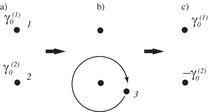
The final state is completely different from the initial one . Indeed, there is no overlap between them, i.e. .
Note that such an exotic phenomenon never occurs if the vortices is boson, fermion, or Abelian anyon. For these cases, the encircling process considered here results in a overall phase at most, so the final state is essentially the same as the initial one. In other words, the above phenomenon is a result of the non-Abelian statistics of vortices. A particle obeying the non-Abelian statistics is called non-Abelian anyon, and a topological phase with non-Abelian anyons is called non-Abelian topological phase.
Up to now, we have focused on the spinless superconductor. Now consider the spinful time-reversal breaking superconductor. An example is a chiral -wave superconductor in Sr2RuO4 or in a 3He A-phase superfluid thin film. When the spin-orbit interaction is negligible and the Cooper pairs preserve a spin in a certain direction, say , the Hamiltonian is given by
with in eq.(3.4). The gap function is given by eq.(3.3). Since is the same as that for the spinless superconductor, the Hilbert space is also the same, that is . Thus the topological number characterizing the state is the same winding number . The difference between the spinless superconductor and the spinful one is the Majorana condition. For the spinful superconductor, the quasiparticle operator
in eq.(3.4) does not satisfy the Majorana condition (3.4). Nevertheless, this does not imply that the Majorana fermion cannot appear in the spinful superconductor. Indeed, in a special kind of vortex called half-quantum vortex, the Majorana fermion appears.
The half-quantum vortex is realized in spinful spin-triplet superconductors, where the spin components of the gap function can rotate around vortex. Using this degrees of freedom, the half-quantum vortex has the following configuration,
| (153) |
where is the -vector of the spin-triplet gap function, the distance from the vortex core, and the angle around the vortex. Since this configuration does not preserve , its BdG Hamiltonian is not given in the form of eq.(3.4). Instead, we can treat the system as two copies of spinless superconductors. Indeed, the matrix representation of the gap function leads to
so there is no mixing between the different spin sectors. Then, each spin sector is the spinless superconductor described by eq.(3.4). (For the down spin sector, and should be replaced by and , respectively.) Equation (3.4) implies that only the down-spin sector has a vortex. Therefore, we can regard as the half quantum vortex as the vortex in spinless superconductor with down spin. This means that if is odd, there is a Majorana zero mode in the half-quantum vortex. Thus the half-quantum vortex can obey the non-Abelian statistics. Recently, an experimental evidence of the half-quantum vortex in Sr2RuO4 has been reported [175]. Also, a half-quantum vortex is expected to exist in a thin film of 3He A phase [176, 177].
3.5 Helical edge modes in TI/QSHE
In this subsection, we consider the band insulators without the superconductivity from the viewpoint of the topology. For time-reversal invariant systems, new topological phases arise when the spin-orbit interaction is strong enough. Here we review briefly such states, the quantum spin Hall states [178, 179, 180, 181] and its three dimensional generalization, topological insulators [182, 183, 184].
The quantum spin Hall state is easily understood as a pair of the integer quantum Hall states if is a good quantum number. Consider the following two-dimensional system preserving ,
where () is the Hamiltonian for up-spin (down-spin) electron. Here we suppose that the spin-orbit interaction works as a kind of magnetic field, and each spin sector realizes an integer quantum Hall state with the Hall conductance (). Due to the time-reversal invariance, the Chern numbers of the two spin sectors are opposite from each other, . Thus, the spin Hall conductance is quantized, while the total Hall conductance, , is zero. Correspondingly, there exist () gapless edge states with up-spin (down-spin) carrying the spin Hall conductance.
Now consider a time-reversal invariant perturbation which does not preserve . The spin indices turns into that of pseudo-spin , and the Chern numbers and are replaced by and . Then, due to the spin mixing, most of the gapless edge states become massive. Nevertheless, if is an odd number, at least one pair of gapless edge states survives: Because of the time-reversal invariance, the gapless states form a set of Kramers doublets. Since there is no mixing in the same Kramers doublet, the Kramers doublets become massive in a pair by the mixing with a different Kramers doublet. Thus, if there are an odd number of the Kramers doublets, which is realized when is odd, at least one Kramers doublet of the gapless edge states remains massless without a partner.
As indicated by the above argument, for a generic time-reversal invariant system, where is not a good quantum number, the quantum spin Hall state is characterized by the parity of , , which is called the invariant in the literature. Then the resultant gapless edge state is called the helical edge mode.
The topological insulator is a three dimensional generalization of the quantum spin Hall state [182, 183, 184]. It is characterized by the four invariants , which can take the value 0 or 1. When, , the system is called strong topological insulator which supports an odd number of 2D Dirac fermions on the surface. When some of , and are 1, while , the system is classified into weak topological insulator. In this case, an even number of Dirac fermions are on the surface, which can in principle be paired and gapped due to the disorder scattering etc., and are not stable. However, the weak topological insulator is still distinct from the conventional insulator with all ’s being zero, as has been evidenced by one-dimensional channels appearing along the dislocation [185].
3.6 Helical superconductors and helical Majorana modes
There exist a topological state of superconductors which is analogous to the quantum spin Hall state. Such a superconductor is called the helical superconductor [155, 158]. A representative example of the helical superconductor is two-dimensional Rashba noncentrosymmetric superconductors [159, 186]. Let us see its basic property.
The model Hamiltonian of the Rashba superconductor in two dimensions is
| (160) |
where () is a creation (an annihilation) operator for an electron with momentum , spin . The energy band dispersion is with the hopping parameter and the chemical potential , and the Rashba spin-orbit coupling is . Because of parity mixing of Cooper pairs, the gap function has both a spin-triplet component and a spin-singlet one at the same time, . Due to the strong spin-orbit coupling, the spin-triplet component is aligned with the Rashba coupling, [187]. For the spin-singlet component , we assume an -wave pairing, . The amplitudes are chosen as real. The Zeeman coupling with a magnetic field in the direction has been also introduced for later use.
Before going to study topological properties of the system, we first examine the bulk spectrum of the system. Topological nature of the system changes only when the gap of the bulk spectrum closes. The bulk spectrum of the system is obtained by diagonalizing the following matrix,
with , and we have
| (165) | |||||
The gap of the system closes only when
| (166) |
which is equivalent to
| (167) |
When , eq.(167) is met either when
| (168) |
or
| (169) |
In the absence of the magnetic field, only eqs.(168) can be met and they are rewritten in simpler forms,
| (170) |
Topological nature of the system does not change unless eq.(168) or eq.(169) (or eq.(170) when ) is satisfied.
When , the system is time-reversal invariant, and the topological property is characterized by the invariant like the quantum spin Hall state. Below, we will show that if the spin-triplet pairing is stronger than the spin-singlet one, the number is non-trivial.
To see this, we adiabatically deform the Hamiltonian of the system without gap closing. This process does not change the topological number, since it changes only when the gap closes [159, 186]. From eq.(170), it is found that if the spin-triplet amplitude is larger than the spin-singlet one on the Fermi surface given by , we can take , then without gap closing. (If at one of the time-reversal momenta , the gap closes when . However, this undesirable gap closing can be avoided by changing or slightly.) Thus, its number is the same as that of the pure spin-triplet SC with . The resultant system preserves , and the BdG Hamiltonian is decomposed into two spinless chiral superconductors in up-spin sector and the down-spin sector, and , respectively,
If the Fermi surface is two-dimensional and electron-like, their Chern numbers is for . (see Fig.27). Thus the number is non-trivial.
From the bulk-edge correspondence, there should exist gapless edges if the spin-triplet pairs dominate the superconductivity. In Fig.29 (a), we show the energy spectrum of the 2D noncentrosymmetric superconductor with edges. It is found that there exist gapless edge states in the bulk gap. The gapless edges states form a Kramers pair.
For comparison, we also illustrate the energy spectrum for the 2D noncentrosymmetric superconductor with purely -wave paring in Fig.29 (b). As is seen clearly, no edge state is obtained. This is also consistent with the trivial number of the purely -wave paring.
We also notice that the helical Majorana gapless edge states are very sensitive to the direction of the applied magnetic field. As seen in Fig.30, they become unstable under a small magnetic field in the -direction, while the gapless edge states are stable under a magnetic field in the - and -direction. As a result, the magnetic field along the edge causes a tiny gap of the order for the edge states. The experimental detection of the edge states have been proposed theoretically [186, 159, 188, 189, 190, 191, 192, 193, 194].


3.6.1 Non-Abelian topological order and Majorana fermion induced by spin-orbit interaction and Zeeman field
The spin-orbit interaction enables us to realize Majorana fermion and non-Abelian topological order in the presence of the Zeeman field [159, 195, 196]. In particular, the Majorana fermion can be realized even if the symmetry of the gap function is spin-singlet dominant [195, 196, 197, 198]. Here we see this interesting phase of noncentrosymmetric superconductors.
An intuitive understanding on this mechanism of non-Abelian topological phase is obtained if we perform the dual transformation of the BdG Hamiltonian [195, 196]. For the two-dimensional Rashba superconductor (160), the dual Hamiltonian is obtained by the following unitary transformation,
which leads to
From eq. (3.6.1), it is found that the Rashba spin-orbit interaction in the original Hamiltonian is formally transformed into a “-wave pairing interaction” with the vector, , in the dual Hamiltonian . Since has a nonstandard constant kinetic term, this does not necessarily mean that the topological properties of are the same as those of a usual -wave superconductor. However, we find that that the topological order emerges when satisfies
| (181) |
due to the Rashba spin-orbit interaction. Indeed, one can prove that the Chern number if the condition (181) is met [159, 195, 196]. Also, the same condition (181) is obtained from the analysis of Majorana zero mode in a vortex [197]. In Fig.31, we illustrate the energy bands of our Hamiltonian (160) with edges. This figure clearly shows the existence of a chiral gapless state if the Zeeman field satisfies eq.(181), even when the spin-triplet superconductor is absent.
From the argument in §3.4, it is evident that a vortex supports a Majorana zero mode in this case. Indeed, we can demonstrate the existence of the Majorana zero mode explicitly by solving the BdG equation for a single vortex [159, 195, 196, 197, 199]. As explained in §3.4, if there exists a single Majorana fermion zero mode for each vortex, vortices obey the non-Abelian statistics. Following ref.[195], we use here the dual Hamiltonian to solve the BdG equation, then construct a solution in the original Hamiltonian by using the duality transformation (3.6.1). For simplicity, we assume and . Then, if satisfies , the low energy properties are governed by quasiparticles on the smaller Fermi surface, which is split from the larger one by the spin-orbit interaction [196]. The larger Fermi surface can be neglected to construct the zero mode. Thus, we concentrate on fermions with for which is decomposed
The BdG equations for with a single vortex can be solved [153], then, we find a unique zero energy solution with a quasiparticle field , where , . The solution is normalizable when eq.(181) is satisfied. This is the Majorana zero energy mode; i.e., . Using the duality transformation (3.6.1), we also found that a vortex in the original Hamiltonian has a single Majorana zero mode, which implies that the vortex is a non-Abelian anyon.
Here note that the condition (181) implies the Zeeman energy larger than the -wave BCS gap . Thus the orbital depairing effect could destroy the superconductivity while the Pauli depairing effect is suppressed in the presence of the Rashba spin-orbit interaction [200, 201]. If the spin-triplet amplitude is dominant and the -wave pair amplitude is small enough, the condition (181) can be met for a weak magnetic field without destroying the superconducting gap [159]. On the other hand, if the -wave pair amplitude is dominant, one always needs a strong magnetic field larger than the superconducting gap. Several schemes to realize the non-Abelian topological phase in this case has been proposed, (i) -wave superfluids in neutral ultracold fermionic atoms with laser generated spin-orbit interaction [195, 196], (ii) heterostructure semiconductor device [197, 202], and (iii) heavy fermion systems [196].
If we consider -wave or -wave pairing instead of the -wave pairing, the condition (181) changes as [198]
| (185) |
since these pair amplitudes vanish at . Thus now the condition (185) is independent of the superconducting gap. This means that the Majorana fermion and the non-Abelian topological phase could be realized in a weak magnetic field without destroying superconductivity for systems with small . In Fig.32, we illustrate the Majorana edge modes in this case. The Majorana fermion state is topologically protected in spite of the presence of bulk gapless nodal excitations. Due to the existence of bulk nodes, one cannot obtain a well-defined Chern number, but the particle-hole symmetry makes the parity of the Chern number well-defined [198]. The non-Abelian nodal superconductor is realizable in an interface between a centrosymmetric nodal superconductor such as high- cuprates and a semiconductor. In such a system, because of the considerably large superconducting gap, the experimental detection of Majorana modes may be easier.


3.6.2 Dispersionless Majorana fermion
For a certain type of noncentrosymmetric superconductors, novel Majorana fermion is possible [203, 204, 161]. It preserves the time-reversal symmetry, however, unlike the helical Majorana fermions, it consists of a single branch of flat dispersion.
The time-reversal invariant Majorana fermion is realized for the -wave Rashba noncentrosymmetric superconductor. Such a pairing symmetry has been suggested for heterointerface LaAlO3/SrTiO3 [205]. Figure 33 illustrates the quasiparticle spectrum for the semi-infinite -wave Rashba noncentrosymmetric superconductor on . Due to the Rashba spin-orbit interaction, the Fermi surface is split into two with the Fermi momenta and (). See Fig.33. There exists a single branch of zero energy edge state in the momentum region between the Fermi surfaces. The wave function for the zero energy edge state can be written as with The Bogoliubov quasiparticle creation operator for this state is constructed in the usual way as , and satisfies the Majorana condition .
Unlike Majorana fermions discussed in previous sections, the present single Majorana bound state at is realized with time-reversal symmetry. The time-reversal invariant Majorana bound state has the following three characteristics. (a) It has a unique flat dispersion: To be consistent with the time-reversal invariance, the single branch of zero mode should be symmetric under . Therefore, by taking into account the particle-hole symmetry as well, the flat dispersion is required. On the other hand, the conventional time-reversal breaking Majorana bound state has a linear dispersion. (b) The spin-orbit coupling is necessary to obtain the time-reversal invariant Majorana bound state. Without spin-orbit coupling, the time-reversal invariant Majorana bound state vanishes. (c) The time-reversal invariant Majorana bound state is topologically stable under small deformations of the Hamiltonian preserving . The topological stability is ensured by the topological invariant [204, 161]
| (186) |
with . The flat dispersion of the Majorana fermion is terminated in a gap node. The last property is closely related to the topological stability of line nodes of noncentrosymmetric superconductors [206, 207].
It is noted that the appearance of surface flat bands in three-dimensional noncentrosymmetric superconductors or topological media have been also discussed recently [208, 209, 210, 211].

3.7 Topological phase in odd-parity superconductors
In §3.4, we have seen that the topological properties of the spinless superconductor changes as the topology of the Fermi surface changes. This is a general property of spin-triplet odd-parity superconductors [163, 212].
To see this, consider a general Hamiltonian for odd-parity superconductors,
where () denotes the creation (annihilation) operator of electron with momentum . The suffix labels other degrees of freedom for electron such as spin, orbital degrees of freedom, sub-lattice indices, and so on. is the Hamiltonian of the electron in the normal state. The system in the normal state is supposed to be invariant under the inversion with , . We also assume that the parity of the gap function is odd,
First, consider the case with the time-reversal symmetry breaking. The BdG Hamiltonian (3.7) has the following particle-hole symmetry,
From this, we can say that if is a quasiparticle state with positive energy satisfying then is a quasiparticle state with negative energy . We use a positive (negative) for to represent a positive (negative) energy quasiparticle state, and set
| (196) |
Let us define the gauge fields
| (197) |
where the relation
| (198) |
holds from (196). In addition, we have
| (199) |
with the unitary matrix given by
| (200) |
where is the -th component of .
Now consider the time-reversal invariant path in the BZ, which passes through the time-reversal invariant momenta and . See Fig.34. Note that is a closed path because of the periodicity of the BZ. The periodicity of the BZ implies that the integration of along is quantized as,
| (201) | |||||
Thus the Berry phases takes only two possible values, and we use it as the topological index,
| (202) |
Like the one-dimensional winding number in §3.3, the topological index characterizes the “one-dimensional gapped superconductor” along the path . When , the bulk-edge correspondence yields that there exists a zero energy edge state at the corresponding momentum in the surface BZ. On the other hand, when , no ZEABS is required at the corresponding momentum in the surface BZ.
Up to now, we have not used the specific property of odd-parity superconductors. For odd-parity superconductors, the combination of the inversion and the electromagnetic gauge symmetry, is manifestly preserved. Thus, has the following symmetry
From this, we have for the time-reversal invariant momentum . Thus, the quasiparticle state at is simultaneously an eigenstate of ,
| (206) |
Then, the product of for occupied states, , has the following interesting properties: (a) it takes only discrete values , and (b) its value can change only when the gap of the system closes at . These properties are what we expect for the topological index, and suggest that is a kind of topological index. Indeed, we can relate to the topological index as [212],
| (207) |
For ordinary superconductors, the superconducting gap is much smaller than the Fermi energy. Therefore, we reasonably assume that the typical energy scale of the gap function at the time-reversal invariant momentum is much smaller than that of . Under this assumption, we can deform the gap function adiabatically so as without closing the bulk energy gap. Because of the topological nature of , this adiabatic process does not change the value of . In the process , the BdG Hamiltonian at reduces to . For this simple Hamiltonian, we can evaluate rather easily, and we obtain the final expression [212],
| (208) |
where is an eigenvalue of and the product of is taken for all eigenstates of . This formula implies that for odd-parity superconductors the gapless boundary state can be predicted by the Fermi surface structure.
When the odd-parity superconductors are fully-gapped in two dimensions, the Chern number also characterizes the topological phases. By using eqs. (54) and (198), it can be linked to the topological index as
| (209) | |||||
where is the upper half of , and is the time-reversal invariant path illustrated in Fig.34(b). Therefore, eq.(208) yields
| (210) |
One can confirm the validity of the formulas (208) and (210) by applying them to the spinless superconductors in Fig.27. For example, from the Fermi surface structures illustrated in the top row, we find that only the case of Fig.27 (b) has an odd Chern number. Correspondingly, a single edge mode appears on each edge in Fig.27 (b). Furthermore, it is found that the difference between Fig.27 (a) and (c) can be understood as the difference in for each case: One find that for Fig. 27 (c), while for (a). The zero energy edge states in (c) are originated from the non-trivial values of these topological indices.

Now consider the time-reversal invariant case. The time-reversal invariance implies that is always trivial, i.e. . However, use of the time-reversal invariance as well as the particle-hole symmetry makes it possible to define another topological index.
Because of the time-reversal invariance, the quasiparticle states form Kramers pairs, , with the time-reversal operator . The new topological index is defined by the gauge field for the “half” of the Kramers doublets, say, . Then the topological index is defined as
| (211) |
In a manner similar to the above, for odd-parity superconductors, are determined by the Fermi surface structure [212],
| (212) |
where is an eigenvalue of , and we have set by using the Kramers degeneracy.
Furthermore, other topological indices characterizing time-reversal invariant superconductors can be linked to the Fermi surface topology. For the full-gapped two-dimensional case, their topological nature is characterized by the number introduced in §3.5 and §3.6. For odd-parity superconductors, it satisfies [163, 212]
| (213) |
where is the time-reversal invariant momenta in Fig.34(b). Thus, we can predict the helical Majorana edge mode from the knowledge of the Fermi surface. In addition, for the full-gapped three-dimensional case, we have another topological index known as the three-dimensional winding number [213, 154, 156, 157]. (When takes a nonzero integer , there exist Majorana cones on the surface.) We can also connect this to the Fermi surface structure as [163, 212, 214]
| (214) |
with in Fig.34 (c). The last formula determines the parity of the three-dimensional winding number, thus it gives a sufficient condition for nonzero . In Fig.34 (d), we illustrate surface states of a three-dimensional time-reversal invariant topological superconductor. The Fermi surface of this model leads to , but and . Consistently, we have two Majorana cones on the surface at the time-reversal invariant points and in the surface Brillouin zone. (For the definition of , see Fig 34(c).)
We would like to emphasis here that the correspondence between the Fermi surface and the gapless surface state discussed in the above are inherent to spin-triplet/odd-parity superconductors. Thus we may identify the spin-triplet/odd-parity superconductivity through the direct measurement of the surface state, irrespective of the details of the gap function [163, 212]. For instance, the formula (214) has been applied to CuxBi2Se3 in order to identify its possible odd-parity superconductivity [214]. Detailed information on ABS for such a material can be predicted by using the formulas (212) and (213) as well.
3.8 Majorana fermion on the surface of topological insulator
As discussed in §3.5, the topological insulator is a new state of matter with time-reversal (symmetry) [178, 179, 215, 180, 181]. Especially, on the surface of the 3D strong topological insulator (STI), there appears odd number of 2D Dirac fermions. Even with a disorder scattering etc., at least one Dirac fermion is protected by the gap and topology of the bulk states and is stable as long as the perturbation is symmetric and does not destroy the bulk gap. In the case of Bi2Se3 and Bi2Te3 [216], there appears only one surface Dirac fermion, which can be regarded as the ”half” of the 2D electrons because the spin direction is determined by the momentum. This ”fractionalization” of the electrons is one of the key concepts in the topologically ordered states. This situation is similar to the case of spinless fermion, and when the Cooper paring occurs, there is a possibility that Majorana fermions will appear [217]. Fu and Kane were the first to study the superconductivity of the surface Dirac fermions of the STI induced by the proximity effect by the superconductors attached to it [218]. Also they considered the ferromagnetic insulator (FI) put on the STI, and its interface with the conventional superconductor (S). They predicted the emergence of the one-dimensional chiral Majorana mode as an Andreev bound state [218]. This situation is similar to that discussed in §3.4. Also by applying the magnetic field, the vortices penetrate the sample. At the core of each vortex, the Majorana bound state is realized at zero energy [218, 219].

Majorana interferometry has been proposed to detect the Majorana fermions [220, 221, 222, 223]. The schematic configuration is shown in Fig.35 . Everything is on top of the STI, and there appears the chiral fermion channel at the interface of two magnetic domains with and magnetization, while the chiral Majorana fermions appear at the interface between FI and S. Let and being the creation and annihilation operators of this chiral fermion. At the branching points, this chiral fermion is connected to the two Majorana edge channels for upper and lower semicircles. Let () be the operator of the Majorana fermion in the upper (lower) semicircle. Let us consider the process that an electron is entering from the left to the branching point described by
| (215) |
At the right branching point, these two Majorana fermions merge into an electron as
| (216) |
or
| (217) |
depending on the even or odd number of vortices () trapped by the superconducting donut according to the Aharanov-Bohm effect. This leads to strong -dependence of the conductance between the left and right leads. Namely, when while when with being an integer. This prediction is based on the fact that the Majorana fermion contains the particle and hole components with equal weight, or an electron is composed of two Majorana fermions.
The other direction of the research is to study the possible manipulation of the Majorana fermion and its relevance to the transport properties in the transverse direction to the interface [224, 225, 226], For that purpose we consider the Hamiltonian for the surface state on STI influenced by the superconductor and ferromagnet ( Fig. 36 ) as given by
where describes the 2D Dirac fermion, and is the magnetic exchange interaction with . Here, , , , denote chemical potential, Pauli matrices, velocity, and magnetization (times the exchange coupling constant which we assume to be 1), respectively [218]. Interestingly, couples to the Dirac fermion as an effective vector potential of the electromagnetic field. For the moment, we assume that the pairing symmetry of superconductor is spin-singlet -wave and is given as and for N/FI/S (Fig. 36 (a)) and S/FI/S (Fig. 36 (b)) junctions formed on the surface of STI, respectively, where denotes the macroscopic phase difference between left and right superconductor. (N represents the normal metal which is the 2D Dirac fermion in the present case.) We also assume that the magnitude of is smaller than that of the bulk energy gap of superconductor deposited on STI because the S/TI interface is not ideal [227].

First, we solved the Andreev bound state (ABS) at the interface of FI/S. As an example, we show in Fig. 37 the energy dispersion as a function of the angle (corresponding to the momentum along the interface) in the right panel, and the corresponding conductance of the N/FI/S junction in the left panel for several values of . Note that the slope of the energy dispersion affects the conductance sensitively. Therefore, it is concluded that the 1D Majorana channel can be controlled by the magnetization of the FI and the chemical potential .

Next, we consider the Josephson effect in S/FI/S junction (Fig. 36(b)). This is mainly due to the tunneling process between the two Majorana edge channels at the two interfaces between S and FI. One interesting prediction is that the current-phase relation can be shifted by the . Figure 38 shows the Josephson current as a function of the phase different between the two superconductors for different values of , where the parallel shift of the curves is seen.

The generalization to the anisotropic pairing superconductors on STI has been discussed in ref.[225, 226] . It is found that the proximity effect to the superconductivity is strongly dependent on the pairing symmetry. For spin-triplet -wave superconductor, there occurs no proximity effect because the spin direction of the 2D Dirac electrons is not consistent with that of the -wave pairing. In the cases of spin-singlet -wave and -wave pairings, there occurs the proximity effect, and the Majorana fermions appear at the interface of FI and S. For spin-singlet -pairing, the zero energy states appear along the edge of the sample even without the magnetization of FI, i.e., without symmetry breaking, which has been well-known. However, the new aspect here is that the zero energy dispersionless bound states are Majorana fermions due to the proximity to STI. With the -component of the magnetization, the Majorana fermion obtains the dispersion, which results in the very different behavior of the conductance compared with the case of spin-singlet -wave superconductors.
4 Discussion
4.1 Interplay between symmetry and topology
| ZEABS | dispersion | top. index | odd- pairing | Majorana | section | |
| No | - | - | No | - | 2.2, 3.3 | |
| Yes | No | OSO | double | 2.2, 3.3 | ||
| Yes | No | OTE | double | 2.2, 3.3 | ||
| chiral (spinless) | Yes | Yes | OTE | chiral | 3.4 | |
| chiral (spinful) | Yes | Yes | OTE | double | 3.4 | |
| () | Yes | Yes | OTE+OSO | helical | 3.6 | |
| () | No | - | - | No | - | 3.6 |
| Yes | No | OSO+OTE | flat | 3.6 |
Up to now, we have studied induced odd-frequency pairings in §2 and topological bulk-edge correspondence in §3. In this section, we discuss the relation between these two.
First, all the known zero energy edge states at the surface of superconductors can be characterized by the topological indices, and are topologically protected. These zero energy states are always associated with the pure odd-frequency pairing at the surface. (When the ABS has the energy dispersion, this statement applies only to the sector of .) In Table 9, we summarize the results for various situations studied thus far.
For -wave superconductor, which belongs to ESE, there is no ZEABS because it is topologically trivial. At the same time, odd-frequency pairing is absent at the surface. However, -wave superconductor, which also belongs to ESE, has ZEABS characterized by the topological index . is the winding number defined for the one-dimensional systems when is fixed as discussed in §3.3. The formation of the ZEABS stems from the sign change of the pair potential felt by injected and reflected quasiparticles. The similar situation occurs for -wave superconductor which belongs to ETO pairing. In these cases, pure odd-frequency pair amplitudes (OSO for , OTE for ) exist at the surface. The ZEABSs can be regarded as double Majorana modes satisfying
| (221) |
Next, we discuss the spinless chiral -wave superconductor where the time-reversal symmetry is broken in the bulk. There exists ABS, however, in contrast to the cases above, it has a dispersion linear in . Because of the broken time-reversal symmetry, it is characterized by the Chern number in a manner similar to the quantum Hall states. The induced odd-frequency pair amplitude at the surface belongs to OTE symmetry. The present ABS is a chiral Majorana mode, which is a genuine Majorana fermion. The case of the spinful chiral -wave superconductor can be regarded as the two copies of the spinless case discussed above. Lastly, the noncentrosymmetric superconductors (NCSs) are discussed. In these superconductors, the parity of the pair amplitudes are mixed. For the case of -wave and -wave mixture, there are two topologically distinct states depending on the relative magnitudes of the corresponding pair potentials. When -wave component is dominant, the ABS is generated as a helical Majorana edge mode. The pair amplitude induced at the surface has OTE+OSO symmetry. The topological index characterizing the ABS is the invariant. On the other hand, when -wave component is dominant, no ABS is generated because it is smoothly connected to the topologically trivial -wave superconductor case without closing the bulk gap. For ()-wave pair potential case, a single branch of dispersionless ABS appears if satisfies some condition. This ZEABS is a single Majorana fermion. The topological index defined by eq.(186) ensures its topological stability [161]. The symmetry of induced odd-frequency pair amplitude is OSO+OTE.
4.2 Related topics
There are several important issues which are not addressed in this review article due to the limited space. We will briefly mention each of them by indicating relevant references.
In this review article, we mainly focus on the interface and surface of superconductors. There are several works on the bulk superconductors from the viewpoint of topology and/or odd-frequency pairings. Non-interacting topological insulators and topological superconductors have been classified based on the universal class of the Anderson localization. [156, 157] The similar results have been reached independently by Kitaev [228] in the framework of K-theory. The classification scheme also has been applied for solitons in topological insulators and topological superconductors.[229] Possible bulk odd-frequency superconductors have been an important issue in many-body physics. Recently, there are several proposals of odd-frequency gap functions in quasi one-dimensional systems [14, 15], magnetic superconductors[230], heavy fermion systems [12, 13], and strongly coupled electron-phonon systems [17]. However, it is noted that the thermodynamic stability and physical properties of the bulk odd-frequency pairing superconductors are still controversial issues [231, 232, 16].
Since superfluid 3He is a well established spin-triplet -wave superfluid, it is natural to expect ABS [23, 24]. ABSs in superfluid 3He have been predicted in the 1980’s [23, 24]. However, the detection of them is not easy since Cooper pairs of superfluid 3He do not have electric charge. Surface ABS of 3He B phase has been observed experimentally by the transverse acoustic impedance [233] in 2005 and specific heat measurements [234] in 2006. In the actual surface of 3He B phase, diffusive scattering by surface roughness plays an important role [235, 236]. When a surface is specular, SABS has a Dirac like linear dispersion which have been recently interpreted as Majorana fermion [155, 237]. There are several theoretical discussions about SABS from the viewpoint of topological superconductivity and Majorana fermions [156, 157, 155, 238, 239, 240, 241, 242]. It is noted that surface Majorana cone has been experimentally observed for highly specular wall of 3He B phase [243, 244]. Surface Majorana ABS (SMABS) has been also discussed in slab geometry of 3He A and B phases [241, 242]. An analogous system of diffusive normal metal/spin-triplet superconductor can be realized in superfluid aerogel/3He hybrid system. Anomalous proximity effects discussed in §2.4 are also expected in the aerogel, since it can be regarded as a diffusive Fermi liquid [245].
Recently, promising candidate of topological superconductor has been discovered in doped topological insulator CuxBi2Se3 [246]. Several experimental [247, 248] and theoretical [214, 249] researches have started. MSABS are also expected in the present new superconductors.
Majorana fermion can be a platform of topological quantum computation. Various systems have been proposed to produce Majorana fermion; spin-triplet -wave superconductors / superfluids [174, 250, 251, 252, 253, 254, 241, 176, 177], fractional quantum Hall system [255], spin singlet -wave superconductor on topological insulator surface with vortex or the interface with ferromagnet [256, 221, 257], noncentrosymmetric superconductors with Zeeman field [258, 196, 198], -wave superfluid of cold atoms with laser generated spin-orbit interaction [195, 196], semiconductor/SC systems including Rashba spin-orbit coupling with FM [197] or Zeeman field [202], one-dimensional system made of 2D QSHS[220] or nanowire[259, 260, 261, 262, 263, 264, 265], quantum anomalous Hall/ SC hybrid system[266, 267], and Half metal /SC system [268, 269].
The detection of Majorana fermion is not a trivial issue since it is a neutral particle. Majorana fermions in condensed matter physics are emergent particles resulting from the many-body interactions of electrons which are charged. Thus, they can be detected through the conversion processes to electron influenced by the phases of the superconducting order parameters. In addition to the Majorana interferometry on topological insulator discussed in §3.8 [220, 221, 222, 223], there are many other proposals for this purpose: (i) Josephson effect [259, 220, 270, 224, 271, 272], (ii) charge transport thorough Majorana fermion [222, 273, 274, 275, 276, 277], (iii) transport noise [278, 279], and (iv) spin anisotropy [159, 237, 238, 280, 204].
4.3 Perspectives
The two major fields opened up in 80’s are the quantum Hall effect and the high- superconductors. The former introduced the concept of topology and the latter the electron correlation in condensed matter physics. The idea of the topology extended to the time-reversal symmetric systems and the topological insulators have been discovered. On the other hand, the electron correlation naturally leads to the anisotropic Cooper pairings with various symmetries. These two streams are now merging into one producing many interesting new directions in the current condensed matter physics.
It is now recognized that there are 3 distinct classes of currents in solids; (i) One is the conventional Ohmic currents with dissipation. (ii) The second is the superconducting currents and/or the superfluid flow with broken gauge symmetry and macroscopic quantum coherence. (iii) The third one is the “topological currents” induced by the nontrivial topology of wavefunctions, and does not require the broken gauge symmetry. The last two have the common feature of dissipationless currents. The last one has not been paid attention thus far, but will be very unique because it can operate at room temperature when the gap protecting the topology is larger than its energy scale.
These three classes have been considered to be rather clearly separated. However, as we have described in this review article, class (ii) and class (iii) are overlapping each other. Namely, there is a class of topological supercurrent at the edge/surface of the superconductors/superfluid. Therefore, the interplay of the broken gauge symmetry and topology offers an intriguing new arena for the future condensed matter physics.
These fundamental understandings of the currents in solids will be essential to develop the electronics in the next generation. The dissipationless operations of devices are the key ingredient for the future applications to electronics, and hopefully the topological supercurrent will serve this goal. The other important issue is the quantum computing. Majorana fermion is regarded as the promising candidate for fault-tolerant qubit. In general, the topological orders bring about the electron fractionalization, which gives the robustness of the quantum states. The three degrees of freedom of electrons, i.e., spin, chirality, particle-antiparticle, can be fractionalized at the edge/surface of topologically ordered bulk states, and chiral Majorana fermions can be regarded as the ultimate fractionalized quantum state. On the other hand, the other direction is to recombine these fractionalized particles into new types of particles [281]. The more the degrees of freedom, the more the system is susceptible to the external stimuli, and hence we can adjust the robustness and sensitivity of the system at will by manipulating the fractionalization/recombination.
To verify these theoretical proposals, experimental progresses are indispensable. There are several relevant experimental techniques such as SR, NMR, neutron scattering, X-ray diffraction, and magneto transport. In particular, the direct observation of edge/surface states by the tunneling spectroscopy and ARPES is highly desired. For more details, the readers are referred to other contributions in this special volume.
Finally, we would like to stress that physics of interface/surface superconductivity includes unexplored quantum phenomena and will be a central topic in condensed matter physics in the decades to come.
Acknowledgements.
The authors thank T. Akazaki, Y. Ando, Y. Asano, A.V. Balatsky, Y. Fominov, S. Fujimoto, A. Furusaki, Y. Fuseya, A.A. Golubov, N. Hayashi, S. Higashitani, M. Ichioka, J. Inoue, S. Kashiwaya, M. Kohmoto, H. Kusunose, J. Linder, Y. Maeno, K. Miyake, T. Mizushima, K. Nagai, S. Onari, M. Oshikawa, X.L. Qi, A. P. Schnyder, R. Shindou, A. Sudbo, Y. Takahashi, Y.Tanuma, M. Ueda, K.Yada, T. Yokoyama, S.C. Zhang for valuable discussions. This work is supported by Grant-in-Aid for Scientifc Research (Grants No. 17071007, No. 17071005, No.19048008, No. 19048015, No. 20654030, No. 22103005(Innovative Areas ”Topological Quantum Phenomena”), No. 22340096, No. 21244053 and No.22540383) from the Ministry of Education, Culture, Sports, Science and Technology of Japan, Strategic International Cooperative Program (Joint Research Type) from Japan Science and Technology Agency, and Funding Program for World-Leading Innovative RD on Science and Technology (FIRST Program).References
- [1] D. Thouless: inThe Quantum Hall Effect, ed. R. E. Prange and S. M. Girvin (Springer-Verlag New York Inc., 1987), p. 101.
- [2] M. Sigrist and K. Ueda: Rev. Mod. Phys. 63 (1991) 239.
- [3] E. Bauer, G. Hilscher, H. Michor, C. Paul, E. Scheidt, A. Gribanov, Y. Seropegin, H. Noël, M. Sigrist, and P. Rogl: Phys. Rev. Lett. 92 (2004) 027003.
- [4] M. Sigrist, D. F. Agterberg, P. A. Frigeri, N. Hayashi, R. P. Kaur, A. Koga, I. Milat, K. Wakabayashi, and Y. Yanase: J. Magn. Magn. Matter. 310 (2007) 536.
- [5] It is noted that the exchange of the two time variables does not mean the time reversal. Therefore the odd-frequency pairing does not mean necessarily the time reversal symmetry breaking.
- [6] V. L. Berezinskii: JETP Lett. 20 (1974) 287.
- [7] A. Balatsky and E. Abrahams: Phys. Rev. B 45 (1992) 13125.
- [8] E. Abrahams, A. Balatsky, D. J. Scalapino, and J. R. Schrieffer: Phys. Rev. B 52 (1995) 1271.
- [9] P. Coleman, A. Georges, and A. M. Tsvelik: J. Phys. Condens. Matter 9 (1997) 345.
- [10] P. Coleman, E. Miranda, and A. Tsvelik: Phys. Rev. B 49 (1994) 8955.
- [11] M. Vojta and E. Dagotto: Phys. Rev. B 59 (1999) R713.
- [12] Y. Fuseya, H. Kohno, and K. Miyake: J. Phys. Soc. Jpn. 72 (2003) 2914.
- [13] T. Hotta: J. Phys. Soc. Jpn. 78 (2009) 123710.
- [14] K. Shigeta, S. Onari, K. Yada, and Y. Tanaka: Phys. Rev. B 79 (2009) 174507.
- [15] K. Shigeta, Y. Tanaka, K. Kuroki, S. Onari, and H. Aizawa: Phys. Rev. B 83 (2011) 140509(R).
- [16] H. Kusunose, Y. Fuseya, and K. Miyake: J. Phys. Soc. Jpn. 80 (2011) 054702.
- [17] H. Kusunose, Y. Fuseya, and K. Miyake: J. Phys. Soc. Jpn. 80 (2011) 044711.
- [18] F. S. Bergeret, A. F. Volkov, and K. B. Efetov: Phys. Rev. Lett. 86 (2001) 4096.
- [19] Y. Tanaka and A. A. Golubov: Phys. Rev. Lett. 98 (2007) 037003.
- [20] Y. Tanaka, A. A. Golubov, S. Kashiwaya, and M. Ueda: Phys. Rev. Lett. 99 (2007) 037005.
- [21] Y. Tanaka, Y. Tanuma, and A. A. Golubov: Phys. Rev. B 76 (2007) 054522.
- [22] M. Eschrig, T. Löfwander, T. Champel, J. Cuevas, and G. Schön: J. Low Temp. Phys. 147 (2007) 457.
- [23] L. J. Buchholtz and G. Zwicknagl: Phys. Rev. B 23 (1981) 5788.
- [24] J. Hara and K. Nagai: Prog. Theor. Phys. 76 (1986) 1237.
- [25] S. Kashiwaya and Y. Tanaka: Rep. Prog. Phys. 63 (2000) 1641.
- [26] T. Löfwander, V. S. Shumeiko, and G. Wendin: Supercond. Sci. Technol. 14 (2001) R53.
- [27] C. R. Hu: Phys. Rev. Lett. 72 (1994) 1526.
- [28] Y. Tanaka and S. Kashiwaya: Phys. Rev. Lett. 74 (1995) 3451.
- [29] M. Matsumoto and H. Shiba: J. Phys. Soc. Jpn 64 (1995) 1703.
- [30] Y. Tanaka and S. Kashiwaya: Phys. Rev. B 53 (1996) 9371.
- [31] Y. Asano, Y. Tanaka, and S. Kashiwaya: Phys. Rev. B 69 (2004) 134501.
- [32] A. F. Andreev: Sov. Phys. JETP 19 (1964) 1228.
- [33] G. E. Blonder, M. Tinkham, and T. Klapwijk: Phys. Rev. B 25 (1982) 4515.
- [34] C. Bruder: Phys. Rev. B 41 (1990) 4017.
- [35] S. Kashiwaya, Y. Tanaka, M. Koyanagi, and K. Kajimura: Phys. Rev. B 53 (1996) 2667.
- [36] S. Kashiwaya, Y. Tanaka, M. Koyanagi, H. Takashima, and K. Kajimura: Phys. Rev. B 51 (1995) 1350.
- [37] S. Kashiwaya, Y. Tanaka, N. Terada, M. Koyanagi, S. Ueno, L. Alff, H. Takashima, Y. Tanuma, and K. Kajimura: J. Phys. Chem. Solid 59 (1998) 2034.
- [38] M. Covington, M. Aprili, E. Paraoanu, L. H. Greene, F. Xu, J. Zhu, and C. A. Mirkin: Phys. Rev. Lett. 79 (1997) 277.
- [39] L. Alff, H. Takashima, S. Kashiwaya, N. Terada, H. Ihara, Y. Tanaka, M. Koyanagi, and K. Kajimura: Phys. Rev. B 55 (1997) R14757.
- [40] J. Y. T. Wei, N.-C. Yeh, D. F. Garrigus, and M. Strasik: Phys. Rev. Lett. 81 (1998) 2542.
- [41] I. Iguchi, W. Wang, M. Yamazaki, Y. Tanaka, and S. Kashiwaya: Phys. Rev. B 62 (2000) R6131.
- [42] A. Biswas, P. Fournier, M. M. Qazilbash, V. N. Smolyaninova, H. Balci, and R. L. Greene: Phys. Rev. Lett. 88 (2002) 207004.
- [43] B. Chesca, H. J. H. Smilde, and H. Hilgenkamp: Phys. Rev. B 77 (2008) 184510.
- [44] Y. Tanaka and S. Kashiwaya: Phys. Rev. B 53 (1996) R11957.
- [45] Y. Tanaka and S. Kashiwaya: Phys. Rev. B 56 (1997) 892.
- [46] Y. S. Barash, H. Burkhardt, and D. Rainer: Phys. Rev. Lett. 77 (1996) 4070.
- [47] S. Kashiwaya, Y. Tanaka, N. Yoshida, and M. R. Beasley: Phys. Rev. B 60 (1999) 3572.
- [48] S. Higashitani: J. Phys. Soc. Jpn. 66 (1997) 2556.
- [49] H. Walter, W. Prusseit, R. Semerad, H. Kinder, W. Assmann, H. Huber, H. Burkhardt, D. Rainer, and J. Sauls: Phys. Rev. Lett. 80 (1998) 3598.
- [50] Y. Tanaka, Y. Asano, A. Golubov, and S. Kashiwaya: Phys. Rev. B 72 (2005) 140503(R).
- [51] M. Yamashiro, Y. Tanaka, and S. Kashiwaya: Phys. Rev. B 56 (1997) 7847.
- [52] M. Yamashiro, Y. Tanaka, Y. Tanuma, and S. Kashiwaya: J. Phys. Soc. Jpn. 67 (1998) 3224.
- [53] X. G. Wen: Quantum Field Theory of Many-Body Systems (Oxford University Press, Oxford, 2004).
- [54] Note that the plateau observed experimentally is explained by the disorder and consequent Anderson localization effect. See for example Chap. 3 of ref.1.
- [55] B. I. Halperin: Phys. Rev. B 25 (1982) 2185.
- [56] Y. Hatsugai: Phys. Rev. Lett. 71 (1993) 3697.
- [57] Y. Hatsugai: J. Phys.: Condens. Matter 9 (1997) 2507.
- [58] M. Z. Hasan and C. L. Kane: Rev. Mod. Phys. 82 (2010) 3045.
- [59] X.-L. Qi and S.-C. Zhang: arXiv:1008.2026 .
- [60] P. W. Anderson: J. Phys. Chem. Solids 26 (1959) 26.
- [61] T. Yokoyama, Y. Tanaka, and A. Golubov: Phys. Rev. B 75 (2007) 134510.
- [62] T. Yokoyama, Y. Tanaka, and A. A. Golubov: Phys. Rev. B 72 (2005) 052512.
- [63] Y. Tanaka, A. A. Golubov, S. Kashiwaya, and M. Ueda: Phys. Rev. Lett. 99 (2007) 037005.
- [64] N. Kopnin: Theory of Nonequilibrium Superconductivity (Oxford University Press, 2001).
- [65] M. Ashida, S. Aoyama, J. Hara, and K. Nagai: Phys. Rev. B 40 (1989) 8673.
- [66] M. Matsumoto and H. Shiba: J. Phys. Soc. Jpn. 64 (1995) 4867.
- [67] J. W. Serene and D. Rainer: Phys. Rep. 101 (1983) 221.
- [68] G. Eilenberger: Z. Phys. 214 (1968) 195.
- [69] M. Eschrig: Phys. Rev. B 61 (2000) 9061.
- [70] W. L. McMillan: Phys. Rev. 175 (1968) 537.
- [71] J. M. Rowell and W. L. McMillan: Phys. Rev. Lett. 16 (1966) 453.
- [72] K. Ichimura and K. Nomura: J. Phys. Soc. Jpn. 75 (2006) 051012.
- [73] F. Laube, G. Goll, H. v. Löhneysen, M. Fogelström, and F. Lichtenberg: Phys. Rev. Lett. 84 (2000) 1595.
- [74] Z. Mao, K. Nelson, R. Jin, Y. Liu, and Y. Maeno: Phys. Rev. Lett. 87 (2001) 037003.
- [75] S. Kashiwaya, H. Kashiwaya, H. Kambara, T. Furuta, H. Yaguchi, Y. Tanaka, and Y. Maeno: Phys. Rev. Lett. 107 (2011) 077003.
- [76] C. Wälti, H. R. Ott, Z. Fisk, and J. L. Smith: Phys. Rev. Lett. 84 (2000) 5616.
- [77] C. S. Turel, J. Y. T. Wei, W. M. Yuhasz, and M. B. Maple: Physica C 463-465 (2007) 32.
- [78] P. M. C. Rourke, M. A. Tanatar, C. S. Turel, J. Berdeklis, C. Petrovic, and J. Y. T. Wei: Phys. Rev. Lett. 94 (2005) 107005.
- [79] Y. Tanaka and A. A. Golubov: Phys. Rev. Lett. 98 (2007) 037003.
- [80] Y. Tanaka, Y. Nazarov, and S. Kashiwaya: Phys. Rev. Lett. 90 (2003) 167003.
- [81] Y. Tanaka, Y. Nazarov, A. Golubov, and S. Kashiwaya: Phys. Rev. B 69 (2004) 144519.
- [82] Y. Tanaka and S. Kashiwaya: Phys. Rev. B 70 (2004) 012507.
- [83] Y. Tanaka, S. Kashiwaya, and T. Yokoyama: Phys. Rev. B 71 (2005) 094513.
- [84] Y. Asano, Y. Tanaka, and S. Kashiwaya: Phys. Rev. Lett. 96 (2006) 097007.
- [85] Y. Asano, Y. Tanaka, A. A. Golubov, and S. Kashiwaya: Phys. Rev. Lett. 99 (2007) 067005.
- [86] T. Yokoyama, Y. Tanaka, and A. A. Golubov: Phys. Rev. B 78 (2008) 012508.
- [87] A. Abrikosov: Superconductivity (Marcel Dekker, New York, 1969).
- [88] G. Blatter, M. V. Feigel’man, V. B. Geshkenbein, A. I. Larkin, and V. M. Vinokur: Rev. Mod. Phys. 66 (1994) 1125.
- [89] C. Caroli, P. G. de Gennes, and J. Matricon: Phys. Lett. 9 (1964) 307.
- [90] H. F. Hess, R. B. Robinson, R. C. Dynes, J. M. Valles, , and J. V. Waszczak: Phys. Rev. Lett. 62 (1989) 214.
- [91] Y. G. Makhlin and G. E. Volovik: JETP Lett. 62 (1995) 737.
- [92] A. I. Larkin and Y. N. Ovchinnikov: Phys. Rev. B 57 (1998) 5457.
- [93] N. B. Kopnin and G. E. Volovik: Phys. Rev. Lett. 62 (1997) 1377.
- [94] G. E. Volovik: JETP Lett. 70 (1999) 609.
- [95] F. Gygi and M. Schlüter: Phys. Rev. B 43 (1991) 7609.
- [96] N. Hayashi, T. Isoshima, M. Ichioka, and K. Machida: Phys. Rev. Lett. 80 (1998) 2921.
- [97] O. Fischer, M. Kugler, I. Maggio-Aprile, C. Berthod, and C. Renner: Rev. Mod. Phys. 79 (2007) 353.
- [98] N. Schopohl and K. Maki: Phys. Rev. B 52 (1995) 490.
- [99] N. Schopohl: arXiv:cond-mat/9804064 .
- [100] Y. Tanaka, H. Takayanagi, and A. Hasegawa: Solid. State Commun. 85 (1993) 321.
- [101] A. S. Mel’nikov and V. M. Vinokur: Nature 415 (2002) 415.
- [102] Y. Tanuma, N. Hayashi, Y. Tanaka, and A. A. Golubov: Phys. Rev. Lett. 102 (2009) 117003.
- [103] Y. Kato: J. Phys. Soc. Jpn. 69 (2000) 3378.
- [104] Y. Kato and N. Hayashi: J. Phys. Soc. Jpn. 71 (2002) 1721.
- [105] N. Hayashi and Y. Kato: J. Low Temp. Phys. 131 (2003) 893.
- [106] Y. Kato and N. Hayashi: Physica C 388-389 (2003) 519.
- [107] T. Yokoyama, M. Ichioka, and Y. Tanaka: J. Phys. Soc. Jpn. 79 (2010) 034702.
- [108] K. D. Usadel: Phys. Rev. Lett. 25 (1970) 507.
- [109] A. Volkov, A. Zaitsev, and T. Klapwijk: Physica C 210 (1993) 21.
- [110] A. Golubov and M. Kupriyanov: J. Low Temp. Phys. 70 (1988) 83.
- [111] W. Belzig, C. Bruder, and G. Schön: Phys. Rev. B 54 (1996) 9443.
- [112] Y. Tanaka, A. A. Golubov, and S. Kashiwaya: Phys. Rev. B 68 (2003) 054513.
- [113] C. Honerkamp and M. Sigrist: J. Low Temp. Phys. 111 (1998) 895.
- [114] W. Belzig, C. Bruder, and G. Schön: Phys. Rev. B 53 (1996) 5727.
- [115] O. Narikiyo and H. Fukuyama: J. Phys. Soc. of Jpn. 58 (1989) 4557.
- [116] S. Higashitani: J. Phys. Soc. Jpn. 66 (1997) 2556.
- [117] Y. S. Barash, M. S. Kalenkov, and J. Kurkijärvi: Phys. Rev. B 62 (2000) 6665.
- [118] H. Walter, W. Prusseit, R. Semerad, H. Kinder, W. Assmann, H. Huber, H. Burkhardt, D. Rainer, and J. Sauls: Phys. Rev. Lett. 80 (1998) 3598.
- [119] Y. Asano, A. A. Golubov, Y. Fominov, and Y. Tanaka: arXiv:1010.1574 .
- [120] F. S. Bergeret, A. F. Volkov, and K. B. Efetov: Rev. Mod. Phys. 77 (2005) 1321.
- [121] F. S. Bergeret, A. F. Volkov, and K. B. Efetov: Phys. Rev. B 68 (2003) 064513.
- [122] A. F. Volkov, Y. V. Fominov, and K. B. Efetov: Phys. Rev. B 72 (2005) 184505.
- [123] A. Kadigrobov, R. I. Shekter, and M. Jonson: Euro Phys. Lett. 90 (2001) 394.
- [124] A. A. Golubov, M. Y. Kupriyanov, and Y. V. Fominov: JETP Lett. 75 (2002) 190.
- [125] A. I. Buzdin: Rev. Mod. Phys. 77 (2005) 935.
- [126] J. Linder, T. Yokoyama, and A. Sudbo: Phys. Rev. B 77 (2008) 174507.
- [127] J. Linder, A. M. Black-Schaffer, and A. Sudbo: Phys. Rev. B 82 (2010) 041409.
- [128] T. Löfwander, T. Champel, J. Durst, and G. Schön: Phys. Rev. Lett. 95 (2005) 187003.
- [129] R. S. Keizer, S. T. B. Goennenwein, T. M. Klapwijk, G. Miao, G.Xiao, and A. Gupta: Nature 439 (2006) 825.
- [130] I. Sosnin, H. Cho, V. T. Petrashov, and A. F. Volkov: Phys. Rev. Lett. 96 (2006) 157002.
- [131] T. S. Khaire, M. A. Khasawneh, J. W. P. Pratt, and N. O. Birge: Phys. Rev. Lett. 104 (2010) 137002.
- [132] W. A. Robinson, J. D. S. Witt, and M. G. Blamire: Science 329 (2010) 59.
- [133] Y. Kalcheim, T. Kirzhner, G. Koren, and O. Millo: Phys. Rev. B 83 (2011) 064510.
- [134] A. Buzdin: Phys. Rev. B 62 (2000) 11377.
- [135] M. Zareyan, W. Belzig, and Y. V. Nazarov: Phys. Rev. Lett 86 (2001) 308.
- [136] I. Baladie and A. Buzdin: Phys. Rev. B 64 (2001) 224514.
- [137] F. S. Bergeret, A. F. Volkov, and K. B. Efetov: Phys. Rev. B 65 (2002) 134505.
- [138] T. Yokoyama, Y. Tanaka, and A. A. Golubov: Phys. Rev. B 72 (2005) 052512.
- [139] T. Yokoyama, Y. Tanaka, and A. A. Golubov: Phys. Rev. B 73 (2006) 094501.
- [140] J. Linder, T. Yokoyama, A. Sudbo, and M. Eschrig: Phys. Rev. Lett. 102 (2009) 107008.
- [141] J. Linder, A. Sudbo, T. Yokoyama, R. Grein, and M.Eschrig: Phys. Rev. B 81 (2010) 214504.
- [142] T. Yokoyama and Y. Tserkovnyak: Phys. Rev. B 80 (2009) 104416.
- [143] T. Yokoyama, Y. Tanaka, and N. Nagaosa: Phys. Rev. Lett. 106 (2011) 246601.
- [144] M. Eschrig, J. Kopu, J. C. Cuevas, and G. Schön: Phys. Rev. Lett. 90 (2003) 137003.
- [145] Y. Asano, Y. Tanaka, and A. A. Golubov: Phys. Rev. Lett. 98 (2007) 107002.
- [146] V. Braude and Y. V. Nazarov: Phys. Rev. Lett. 98 (2007) 077003.
- [147] M. Eschrig and T. Löfwander: Nature Physics 4 (2008) 138.
- [148] Y. Asano, Y. Sawa, Y. Tanaka, and A. A. Golubov: Phys. Rev. B 76 (2007) 224525.
- [149] S. Takahashi, S. Hikino, M. Mori, J. Martinek, and S. Maekawa: Phys. Rev. Lett. 99 (2007) 057003.
- [150] M. S. Anwar, F. Czeschka, M. Hesselberth, M. Porcu, and J. Aarts: Phys. Rev. B 82 (2010) 100501(R).
- [151] D. J. Thouless, M. Kohmoto, M. P. Nightingale, and M. den Nijs: Phys. Rev. Lett. 49 (1982) 405.
- [152] M. Kohmoto: Ann. Phys. 160 (1985) 343.
- [153] N. Read and D. Green: Phys. Rev. B 61 (2000) 10267.
- [154] G.R.Volovik: The Universe in a Helium Droplet (Oxford Science Publications, 2003).
- [155] X. L. Qi, T. L. Hughes, S. Raghu, and S. C. Zhang: Phys. Rev. Lett. 102 (2009) 187001.
- [156] A. P. Schnyder, S. Ryu, A. Furusaki, and A. W. W. Ludwig: Phys. Rev. B 78 (2008) 195125.
- [157] S. Ryu, A. P.Schnyder, A. Furusaki, and A. Ludwig: New J. Phys. 12 (2010) 065010.
- [158] R. Roy: arXiv:0803.2881 .
- [159] M. Sato and S. Fujimoto: Phys. Rev. B 79 (2009) 094504.
- [160] M. Sato: Bussei Kenkyu 94 (2010) 311.
- [161] M. Sato, Y. Tanaka, K. Yada, and T. Yokoyama: Phys. Rev. B 83 (2011) 224511.
- [162] S. Ryu and Y. Hatsugai: Phys. Rev. Lett. 89 (2002) 077002.
- [163] M. Sato: Phys. Rev. B 79 (2009) 214526.
- [164] For the index theorem, see for example ref.[282].
- [165] Note that is different from in ref.[161] by a factor while they are essentially the same topological index.
- [166] J. Goryo and K. Ishikawa: Phys. Lett. A 260 (1999) 294.
- [167] A. Furusaki, M. Matsumoto, and M. Sigrist: Phys. Rev. B 64 (2001) 054514.
- [168] Here we implicitly assume that at with . If this is not the case, one needs to deform the gap function slightly to satisfy the assumption. After this regulaization, one can apply the formula. This prescription does not change the value of the topological index.
- [169] R. Roy: Phys. Rev. Lett. 105 (2010) 186401.
- [170] N. B. Kopnin and M. M. Salomaa: Phys. Rev. B 44 (1991) 9667.
- [171] T. Fukui and T. Fujiwara: J. Phys. Soc. Jpn. 79 (2010) 033701.
- [172] T. Fukui and T. Fujiwara: Phys. Rev. B 82 (2010) 184536.
- [173] L. Santos, Y. Nishida, C. Chamon, and C. Mudry: Phys. Rev. B 83 (2011) 104522.
- [174] D. A. Ivanov: Phys. Rev. Lett. 86 (2001) 268.
- [175] J. Jang, D. G. Ferguson, V. Vakaryuk, R. Budakian, S. B. Chung, P. M. Goldbart, and Y. Maeno: Science 331 (2011) 186.
- [176] T. Kawakami, Y. Tsutsumi, and K. Machida: Phys. Rev. B 79 (2009) 092506.
- [177] T. Kawakami, T. Mizushima, and K. Machida: J. Phys. Soc. Jpn. 80 (2011) 044603.
- [178] C. L. Kane and E. J. Mele: Phys. Rev. Lett. 95 (2005) 146802.
- [179] C. L. Kane and E. J. Mele: Phys. Rev. Lett. 95 (2005) 226801.
- [180] B. A. Bernevig and S. C. Zhang: Phys. Rev. Lett. 96 (2006) 106802.
- [181] B. A. Bernevig, T. L. Hughes, and S. C. Zhang: Science 314 (2006) 1757.
- [182] L. Fu, K. C. L, and E. J. Mele: Phys. Rev. Lett. 98 (2007) 106803.
- [183] J. E. Moore and L. Balents: Phys. Rev. B 75 (2007) 121306(R).
- [184] R. Roy: Phys. Rev. B 79 (2009) 195322.
- [185] Y. Ran, Y. Zhang, and A. Vishwanath: Nature Physics 5 (2009) 298.
- [186] Y. Tanaka, T. Yokoyama, A. V. Balatsky, and N. Nagaosa: Phys. Rev. B 79 (2009) 060505.
- [187] P. A. Frigeri, D. F. Agterberg, A. Koga, and M. Sigrist: Phys. Rev. Lett. 92 (2004) 097001.
- [188] T. Yokoyama, Y. Tanaka, and J. Inoue: Phys. Rev. B 72 (2005) 220504(R).
- [189] C. Iniotakis, N. Hayashi, Y. Sawa, T. Yokoyama, U. May, Y. Tanaka, and M. Sigrist: Phys. Rev. B 76 (2007) 012501.
- [190] M. Eschrig, C. Iniotakis, and Y. Tanaka: arXiv:1001.2486 .
- [191] A. Vorontsov, I. Vekhter, and M. Eschrig: Phys. Rev. Lett. 101 (2008) 127003.
- [192] C. Lu and S. Yip: Phys. Rev. B 80 (2009) 024504.
- [193] A. P. Schnyder, P. M. R. Brydon, D. Manske, and C. Timm: Phys. Rev. B 82 (2010) 184508.
- [194] A. P. Schnyder, S. Ryu, and A. W. W. Ludwig: Phys. Rev. Lett. 102 (2009) 196804.
- [195] M. Sato, Y. Takahashi, and S. Fujimoto: Phys. Rev. Lett. 103 (2009) 020401.
- [196] M. Sato, Y. Takahashi, and S. Fujimoto: Phys. Rev. B 82 (2010) 134521.
- [197] J. D. Sau, R. M. Lutchyn, S. Tewari, and S. D. Sarma: Phys. Rev. Lett. 104 (2010) 040502.
- [198] M. Sato and S. Fujimoto: Phys. Rev. Lett. 105 (2010) 217001.
- [199] J. D. Sau, S. Tewari, R. Lutchyn, T. Stanescu, and S. D. Sarma: Phys. Rev. B 82 (2010) 214509.
- [200] P. A. Frigeri, D. F. Agterberg, A. Koga, and M. Sigrist: Phys. Rev. Lett. 92 (2004) 097001.
- [201] S. Fujimoto: J. Phys. Soc. Jpn. 76 (2007) 051008.
- [202] J. Alicea: Phys. Rev. B 81 (2010) 125318.
- [203] Y. Tanaka, Y. Mizuno, T. Yokoyama, K. Yada, and M. Sato: Phys. Rev. Lett. 105 (2010) 097002.
- [204] K. Yada, M. Sato, Y. Tanaka, and T. Yokoyama: Phys. Rev. B. 83 (2011) 064505.
- [205] K. Yada, S. Onari, Y. Tanaka, and J. Inoue: Phys. Rev. B 80 (2009) 140509.
- [206] M. Sato: Phys. Rev. B 73 (2006) 214502.
- [207] B. Béri: Phys. Rev.B 81 (2010) 134515.
- [208] A. P. Schnyder and S. Ryu: arXiv:1011.1438 .
- [209] P. M. R. Brydon, A. P. Schnyder, and C. Timm: arXiv:1104.2257 .
- [210] T. T. Heikkilä and G. E. Volovik: JETP Lett. 93 (2011) 59.
- [211] T. T. Heikkilä, N. B. Kopnin, and G. E. Volovik: arXiv:1012.0905 .
- [212] M. Sato: Phys. Rev. B 81 (2010) 220504(R).
- [213] P. Grinevich and G. E. Volovik: J. Low Temp. Phys. 72 (1988) 371.
- [214] L. Fu and E. Berg: Phys. Rev. Lett. 105 (2010) 097001.
- [215] L. Fu and C. L. Kane: Phys. Rev. B 74 (2006) 195312.
- [216] For review, see refs.[58] and [59].
- [217] A. Kitaev: Ann. Phys. 321 (2006) 2.
- [218] L.Fu and C. L. Kane: Phys. Rev. Lett. 100 (2008) 096407.
- [219] A similar Majorana bound state in a vortex and its non-Abelian statistics for an -wave superconducting state have been discussed for the first time in ref.[283] in a different context. For the relation to Fu-Kane model, see also appendix E in ref.[196].
- [220] L. Fu and C. L. Kane: Phys. Rev. Lett. 102 (2009) 216403.
- [221] A. R. Akhmerov, J. Nilsson, and C. W. J. Beenakker: Phys. Rev. Lett. 102 (2009) 216404.
- [222] K. T. Law, P. A. Lee, and T. K. Ng: Phys. Rev. Lett. 103 (2009) 237001.
- [223] C. Benjamin and J. K. Pachos: Phys. Rev. B 81 (2010) 085101.
- [224] Y. Tanaka, T. Yokoyama, and N. Nagaosa: Phys. Rev. Lett. 103 (2009) 107002.
- [225] J. Linder, Y. Tanaka, T. Yokoyama, A. Sudbo, and N. Nagaosa: Phys. Rev. Lett. 104 (2010) 067001.
- [226] J. Linder, Y. Tanaka, T. Yokoyama, A. Sudbo, and N. Nagaosa: Phys. Rev. B 81 (2010) 184525.
- [227] G. Fagas, G. Tkachov, A. Pfund, and K. Richter: Phys. Rev. B 71 (2005) 224510.
- [228] A. Kitaev: AIP Conf. Proc. 1134 (2009) 22.
- [229] J. C. Y. Teo and C. L. Kane: Phys. Rev. B 82 (2010) 11512.
- [230] K. Shigeta, S. Onari, and Y. Tanaka: arXiv:1104.4693 .
- [231] D. Solenov, I. Martin, and D. Mozyrsky: Phys. Rev. B 79 (2009) 132502.
- [232] Y. Fuseya and K. Miyake: J. Phys. Soc. Jpn. 80 (2011) 054705.
- [233] Y. Aoki, Y. Wada, M. Saitoh, R. Nomura, Y. Okuda, Y. Nagato, M. Yamamoto, S. Higashitani, and K. Nagai: Phys. Rev. Lett. 95 (2005) 075301.
- [234] H. Choi, J. P. Davis, J. Pollanen, and W. P. Halperin: Phys. Rev. Lett. 96 (2006) 125301.
- [235] Y. Nagato, M. Yamamoto, and K. Nagai: J. Low Temp. Phys 110 (1998) 1135.
- [236] K. Nagai, Y. Nagato, M. Yamamoto, and S. Higashitani: J. Phys. Soc. Jpn. 77 (2008) 111003.
- [237] B. Chung and S. C. Zhang: Phys. Rev. Lett. 103 (2009) 235301.
- [238] Y. Nagato, S. Higashitani, and K. Nagai: J. Phys. Soc. Jpn. 78 (2009) 123603.
- [239] G. Volovik: JETP Lett. 90 (2009) 587.
- [240] G. Volovik: JETP Lett. 90 (2009) 398.
- [241] Y. Tsutsumi, T. Mizushima, M. Ichioka, and K. Machida: J. Phys. Soc. Jpn. 79 (2010) 113601.
- [242] Y. Tsutsumi, M. Ichioka, and K. Machida: Phys. Rev. B 83 (2011) 094510.
- [243] S. Murakawa, Y. Tamura, Y. Wada, M. Wasai, M. Saitoh, Y. Aoki, R. Nomura, Y. Okuda, Y. Nagato, M. Yamamoto, S. Higashitani, and K. Nagai: Phys. Rev. Lett. 103 (2009) 155301.
- [244] S. Murakawa, Y. Wada, Y. Tamura, M. Wasai, M. Saitoh, Y. Aoki, R. Nomura, Y. Okuda, Y. Nagato, M. Yamamoto, S. Higashitani, and K. Nagai: J. Phys. Soc. Jpn. 80 (2011) 013602.
- [245] S. Higashitani, Y. Nagato, and K. Nagai: J. Low Temp. Phys. 155 (2009) 83.
- [246] Y. Hor, A. Williams, J. Checkelsky, P.Roushan, J.Seo, Q.Xu, H. Zandbergen, A.Yazdani, N. Ong, and R. Cava: Phys. Rev. Lett 104 (2010) 057001.
- [247] L. A. Wray, S. Y. Xu, Y. Xia, Y. S. Hor, D. Qian, A. V. Fedorov, H. Lin, A. Bansil, R. J. Cava, and M. Z. Hasan: Nature Phys. 6 (2010) 855.
- [248] M. Kriener, K. Segawa, Z. Ren, S. Sasaki, and Y. Ando: Phys.Rev. Lett. 106 (2011) 127004.
- [249] L. Hao and T. K. Lee: Phys.Rev. Lett. 83 (2011) 134516.
- [250] S. Tewari, S. D. Sarma, C. Nayak, C. Zhang, and P. Zoller: Phys. Rev. Lett. 98 (2007) 010506.
- [251] T. Mizushima, M. Ichioka, and K. Machida: Phys. Rev. Lett. 101 (2008) 150409.
- [252] C. Zhang, S. Tewari, R. M. Lutchyn, and S. D. Sarma: Phys. Rev. Lett. 101 (2008) 160401.
- [253] N. R. Cooper and G. V. Shlyapnikov: Phys. Rev. Lett. 103 (2009) 155302.
- [254] T. Mizushima and K. Machida: Phys. Rev. A 81 (2010) 053605.
- [255] G. Moore and N. Read: Nucl. Phys. B 360 (1991) 362.
- [256] L.Fu and C. L. Kane: Phys. Rev. Lett. 100 (2008) 096407.
- [257] T. Neupert, S. Onoda, and A. Furusaki: Phys. Rev. Lett. 105 (2010) 206404.
- [258] S. Fujimoto: Phys. Rev. B 77 (2008) 220501(R).
- [259] A. Y. Kitaev: Usp. Fiz. Nauk (Suppl.) 171 (2001) 131.
- [260] R. M. Lutchyn, T. Stanescu, and S. D. Sarma: Phys. Rev. Lett. 106 (2011) 127001.
- [261] Y. Oreg, G. Refael, and F. von Oppen: arXiv:1003.1145 .
- [262] J. Alicea, Y. Oreg, G. Refael, F. von Oppen, and M. P. A. Fisher: arXiv:1006.4395 .
- [263] P. W. Brouwer, M. Duckheim, A. Romito, and F. von Oppen: arXiv:1103.2746 .
- [264] P. W. Brouwer, M. Duckheim, A. Romito, and F. von Oppen: arXiv:1104.1531 .
- [265] J. D. Sau, C. H. Lin, H.-Y. Hui, and S. D. Sarma: arXiv:1103.2770 .
- [266] X. L. Qi, T. L. Hughes, and S. C. Zhang: Phys. Rev. B 82 (2010) 184516.
- [267] A. Ii, K. Yada, M. Sato, and Y. Tanaka: Phys. Rev. B 83 (2011) 224524.
- [268] S. B. Chung, H.-J. Zhang, X.-L. Qi, and S.-C. Zhang: arXiv:1011.6422 .
- [269] P. A. Lee: arXiv:0907.2681v2 .
- [270] R. M. Lutchyn, T. Stanescu, and S. D. Sarma: Phys. Rev. Lett. 105 (2010) 077001.
- [271] Y. Asano, Y. Tanaka, and N. Nagaosa: Phys. Rev. Lett. 105 (2010) 056402.
- [272] D. I. Pikulin and Y. V. Nazarov: arXiv:1103.0780 .
- [273] K. Flensberg: Phys. Rev. B 82 (2010) 180516(R).
- [274] V. Shivamoggi, G. Refael, and J. E. Moore: Phys. Rev. B 82 (2010) 041405(R).
- [275] L. Fu: Phys. Rev. Lett. 104 (2010) 056402.
- [276] I. Serban, B. Beri, A. R. Akhmerov, and C. W. J. Beenakker: Phys. Rev. Lett. 104 (2010) 147001.
- [277] B. Beri: arXiv:1102.4541 .
- [278] S. B. Chung, X.-L. Qi, J. Maciejko, and S.-C. Zhang: Phys. Rev. B 83 (2011) 100512.
- [279] A. Golub and B. Horovitz: arXiv:1101.3025 .
- [280] R. Shindou, A. Furusaki, and N. Nagaosa: Phys. Rev. B 82 (2010) 180505.
- [281] Y. Tanaka and N. Nagaosa: Phys. Rev. Lett. 103 (2009) 166403.
- [282] M. Nakahara: Geometry, Topology and Physics (Institute of Physics Publishing, Bristol and Philadelphia, 2003).
- [283] M.Sato: Phys. Lett. B 575 (2003) 126.