A Froggatt-Nielsen Model for
Leptophilic Scalar Dark Matter Decay
Abstract
We construct a model of decaying, TeV-scale scalar dark matter motivated by data from the PAMELA and Fermi-LAT experiments. By introducing an appropriate Abelian discrete symmetry and an intermediate scale of vector-like states that are responsible for generating lepton Yukawa couplings, we show that Planck-suppressed corrections may lead to decaying dark matter that is leptophilic and has the desired lifetime. The dark matter candidate decays primarily to lepton/anti-lepton pairs, and at a subleading rate to final states with a lepton, anti-lepton and standard model Higgs boson. We show that the model can reproduce the observed positron flux and positron fraction while remaining consistent with the bounds on the cosmic ray antiproton flux.
I Introduction
A number of earth-, balloon-, and satellite-based experiments have observed anomalies in the spectra of cosmic ray electrons and positrons. Fermi-LAT [1] and H.E.S.S. [2] have measured an excess in the flux of electrons and positrons up to, and beyond TeV, respectively. PAMELA [3], which is sensitive to electrons and positrons up to a few hundred GeV in energy, detects an upturn in the positron fraction beginning around 7 GeV, in disagreement with the expected decline from secondary production mechanisms. Recent measurements at Fermi-LAT support this result [4]. In contrast, current experiments observe no excess in the proton or antiproton flux [5]. Although astrophysical explanations are possible [6], these observations can be explained if the data includes a contribution from the decays of unstable dark matter particles that populate the galactic halo [7]. The dark matter candidate must be TeV-scale in mass, have a lifetime of order seconds, and decay preferentially to leptons. A number of scenarios have been proposed to explain the desired dark matter lifetime and decay properties [8, 9, 10, 11, 12].
To be more quantitative, consider a scalar dark matter candidate which (after the breaking of all relevant gauge symmetries) has an effective coupling to some standard model fermion given by To obtain a lifetime of seconds, one finds if TeV. From the perspective of naturalness, the origin of such a small dimensionless number requires an explanation. One possibility is that physics near the dark matter mass scale is entirely responsible for the appearance of a small number, as is the case in models where a global symmetry, that would otherwise stabilize the dark matter candidate, is broken by instanton effects of a new non-Abelian gauge group . A leptophilic model of fermionic dark matter along these lines was presented in Ref. [8]: the new gauge group is broken not far above the dark matter mass scale and the effective coupling is exponentially suppressed, , where is the gauge coupling. (An example of a supersymmetric model with anomaly-induced dark matter decays can be found in Ref. [9].) On the other hand, the appearance of a small effective coupling can arise if the breaking of the stabilizing symmetry is communicated to the dark matter via higher-dimension operators suppressed by some high scale . Then it is possible that is suppressed by , for some power ; it is well known that for TeV and , the correct lifetime can be obtained for GeV, remarkably coincident with the grand unification (GUT) scale in models with TeV-scale supersymmetry (SUSY) [10]. If the LHC fails to find SUSY in the coming years, however, then the association of GeV with a fundamental mass scale will no longer be strongly preferred. Exploring other alternatives is well motivated from this perspective and, in any event, may provide valuable insight into the range of possible decaying dark matter scenarios.
The very naive estimate for discussed above presumes that the result is determined by a TeV-scale dark matter mass , a single high scale and no small dimensionless factors. Given these assumption, the choice , where GeV is the reduced Planck mass, would not be viable: the dark matter decay rate is much too large for (i.e., there would be no dark matter left at the present epoch) and is much too small for (i.e., there would not be enough events to explain the cosmic ray excess). However, Planck-suppressed effects arise so generically that we should be careful not to discount them too quickly. What we show in the present paper is that Planck-suppressed operators can lead to the desired dark matter lifetime if they correct new physics at an intermediate scale. In the model that we present, this is the scale at which Yukawa couplings of the standard model charged leptons are generated via the integrating out of vector-like states. This sector will have the structure of a Froggatt-Nielsen model [13]: an Abelian discrete symmetry will restrict the couplings of the standard model leptons and the vector-like states, but will be spontaneously broken by the vacuum expectation values (vevs) of a set of scalar fields . Integrating out the heavy states will not only lead to the standard model charged lepton Yukawa couplings, but also to dark matter couplings that are naturally leptophilic and lead to dark matter decay. Aside from setting the overall scale of the charged lepton masses, the symmetry structure of our model will not restrict the detailed textures of the standard model Yukawa matrices. This feature is not automatic; symmetries introduced to guarantee dark matter leptophilia may also make it difficult to obtain the correct lepton mass matrices, at least without additional theoretical assumptions (for example, the addition of electroweak Higgs triplets, as in the model of Ref. [12]). Our framework is free of such complications and is compatible, in principle, with many possible extensions that might address the full flavor structure of the standard model.
Our paper is organized as follows. In the next section, we present a model that illustrates our proposal. In Section 3, we compute the predicted flux, , and the positron fraction for some points in the parameter space of our model and compare our results to the relevant cosmic ray data. It is worth noting that this analysis has applicability to any model that leads to similar dark matter decay operators. In Section 4, we comment on the relic density and dark matter direct detection in our example model. In Section 5, we summarize our conclusions.
II A Model
We assume that the right-handed charged leptons of the standard model, , and four sets of heavy vector-like charged leptons are constrained by the discrete symmetry
| (1) |
with and to be determined shortly. We assume that the vector-like leptons have the same electroweak quantum numbers as
| (2) |
All the fields shown are assumed to be triplets in generation space, with their generation indices suppressed. Under the discrete symmetry, the fields in Eq. (2) are taken to transform as
| (3) |
| (4) |
We will take and to be elements of and , respectively, with and . In addition, we assume the presence of a heavy right-handed neutrino, , that is a singlet under . We note that the fields that are charged under do not transform under any of the non-Abelian standard model gauge group factors, so that satisfies the consistency conditions of a discrete gauge symmetry in the low-energy theory [14]; such discrete symmetries are not violated by quantum gravitational effects11 1 The consistency conditions require that anomalies involving the non-Abelian gauge groups that are linear in a continuous group that embeds must vanish, as is automatic above. Ref. [14] indicates that no rigorous proof exists that the cancellation of the linear gravitational anomalies is a necessary condition for the consistency of the low-energy theory. Nonetheless, such a cancellation can be achieved here by including a singlet, left-handed fermion, , that transforms in the same way as under . For the choice , adopted later in this section, can develop a Majorana mass somewhat below and decay rapidly to lighter states via Planck-suppressed operators. Including such a state does not affect the phenomenology of the model otherwise.. The Yukawa couplings of the standard model charged leptons arise when the symmetry is spontaneously broken and the vector-like leptons are integrated out of the theory. Symmetry breaking is accomplished via the vacuum expectation values of two scalar fields and , which transform as
| (5) |
The following renormalizable Lagrangian terms involving the charged lepton fields are allowed by the discrete symmetry:
| (6) | |||||
While it is not our goal to produce a theory of flavor, we note that the terms in Eq. (6) are of the type one expects in flavor models based on the Froggatt-Nielsen mechanism. Hence, integrating out the fields leads to a higher-dimension operator
| (7) |
which provides an origin for the charged lepton Yukawa couplings. Choosing gives the correct scale for the tau lepton Yukawa coupling; the smaller, electron and muon Yukawa couplings may be accommodated by suitable choices of the undetermined couplings in Eq. (6). One might imagine that the remaining Yukawa hierarchies could be arranged by the imposition of additional symmetries, though we will not explore that possibility here.
We now introduce our dark matter candidate , a complex scalar field that transforms as
| (8) |
under . We assume that all the nonvanishing powers of and shown in Eqs. (3), (4) and (8) are nontrivial, which requires that and . Then, there are no renormalizable interactions involving a single field (or its conjugate) and two fermionic fields that could lead to dark matter decay. However, non-renormalizable, Planck-suppressed operator provide the desired effect. The lowest-order, Planck-suppressed correction to Eqs. (6) that involves a single field is the unique dimension-six operator
| (9) |
Including Eq. (9) and again integrating out the heavy, vector-like states, one obtains a new higher-dimension operator,
| (10) |
which leads to dark matter decay. For TeV (compatible qualitatively with fits to the PAMELA and Fermi-LAT data), a lifetime of seconds is obtained when
| (11) |
For our operator expansion to be sensible, we require ; however, we also do not want a proliferation of wildly dissimilar physical scales, if this can be avoided. Interestingly, if we choose to be the geometric mean of and , one finds
| (12) |
which meets our aesthetic requirements. Standard model quark and neutral lepton masses are unaffected by the discrete symmetry of our model, by construction. Light neutrino masses arise via a conventional see-saw mechanism, and it is possible to obtain a right-handed neutrino mass scale , so that all the heavy leptons appear at a comparable scale. Assuming that the largest neutrino squared mass is comparable to eV2, as suggested by atmospheric neutrino oscillations [15], then this possibility is obtained if the overall scale of the Yukawa coupling matrix that appears in the neutrino Dirac mass term is of the same order as the charm quark Yukawa coupling.

This scenario is depicted in Fig. 1. In this case, the theory is characterized by three fundamental scales: the Planck scale, an intermediate scale (associated with charged lepton flavor and right-handed neutrino masses), and the TeV-scale. Symmetry-breaking vevs appear within a factor of below the latter two. Of course, the right-handed neutrino scale need not be linked with the scale at which the charged lepton Yukawa couplings are generated; this is simply one of many viable possibilities that depend on choices of the free parameters of the model.
Finally, we return to the discrete symmetry group . We have noted that the structure of the theory that we have described is obtained for and , but this does not take into account an important additional constraint: there must be no Planck-suppressed operators involving couplings between the various scalar fields in the theory that can lead to other dark matter decay channels that are either (i) too fast or (ii) too hadronic. For example, the choice and , allows the renormalizable -invariant operator , which leads to mixing, for example, between the and fields; the latter couples to two standard model leptons via the operator in Eq. (7), leading to a disastrously large decay rate. We find that all unwanted operators are sufficiently suppressed if we take and , that is
| (13) |
The lowest-order combination of scalar fields that is invariant under , as well as the standard model gauge group, is
| (14) |
Suppression by three factors of the Planck scale is more than sufficient to suppress any operators that are generated when the and fields are integrated out of the theory, or that may be constructed from products of Eq. (14) with any -singlet, gauge-invariant combination of standard model fields. It is straightforward to confirm that the alternative choice
| (15) |
is also viable, by similar arguments. The difference between the symmetry groups and is that the former allows two types of dark matter mass terms: and . This leads to a mass splitting between the two real scalar components of , so that the lighter is the dark matter candidate. The choice forbids the mass terms, so that the dark matter consists of particles and anti-particles associated with the original complex scalar field. We note that in this theory, the renormalizable interactions involving have an accidental U(1)χ global symmetry which would lead to dark matter stability in the absence of the Planck-suppressed effects. The analysis that we present in the following sections is somewhat simplified by the choice of , which we adopt henceforth.
III Cosmic Ray Spectra
In this section, we investigate the cosmic ray and proton/antiproton spectra of our model. Our treatment of cosmic ray propagation follows that of Ref. [16]. We show that model parameters may be chosen to accommodate the positron excess and the rising electron-positron flux observed by the PAMELA and Fermi-LAT experiments, respectively.
In Eq. (10), we identified the operator responsible for dark matter decays. More explicitly, this operator may be written
| (16) |
where and are generation indices, and represents unknown order-one coefficients. Different choices for the couplings will lead, in principle, to different cosmic ray spectra. To simplify the analysis, we focus on two possibilities: In the lepton mass eigenstate basis, the fermions appearing in the decay operators are either (i) muons exclusively, or (ii) taus exclusively. We will find that either of these choices is consistent with the data, even though we have not fully exploited the parametric freedom available in the . This is sufficient to demonstrate the viability of our model. The remaining factors in the operator coefficient are chosen to obtain the desired dark matter lifetime, as we discussed in the previous section.
In unitary gauge, the operator (16) can be be expanded
| (17) |
where is the standard model Higgs field, which we will assume has a mass of GeV, GeV, and . The term proportional to the Higgs vev leads to the two-body decay , for or , while the remaining term contributes to . We take both of these decay channels into account in our numerical analysis. The final state particles in these primary decays will subsequently decay. The electrons, positrons, protons and antiprotons that are produced must be added to expected astrophysical backgrounds to predict the spectra at experiments like PAMELA and Fermi-LAT.
Electrons and positrons that are produced in dark matter decays must propagate through the Milky Way before reaching the Earth. In order to determine the observed fluxes, one must model this propagation. The transport equation for electron and positrons is given by
| (18) |
where is the number density of electron or positrons per unit energy, is the diffusion coefficient and is the energy loss rate. We assume the MED propagation model described in Ref. [17]. The diffusion coefficient and the energy loss rate are assumed to be spatially constant throughout the diffusion zone and are given by
| (19) |
and
| (20) |
where GeV. The last term in Eq. (18) is the source term given by
| (21) |
where is the dark matter mass and is the dark matter lifetime. In models like ours, where the dark matter can decay via more than one channel, the energy spectrum is given by
| (22) |
where is the branching fraction and is the electron-positron energy spectrum of the decay channel. We use PYTHIA [18] to determine the . For the dark matter density, , we adopt the spherically symmetric Navarro-Frenk-White halo density profile [19]
| (23) |
with and . The solutions to the transport equation are subject to the boundary condition at the edge of the diffusion zone, a cylinder of half-height kpc and radius kpc measured from the galactic center.
The solution of the transport equation can be written
| (24) |
where is a Green’s function, whose explicit form can be found in Ref. [20]. The interstellar flux then follows immediately from
| (25) |
We adopt a parameterization of the interstellar background fluxes given in Ref. [16]:
| (26) |
| (27) |
Finally, the flux at the top of the earth’s atmosphere, , is corrected by solar modulation effects [16],
| (28) |
where , and MeV. and are the energy of positron/electron at the heliospheric boundary and at the top of atmosphere, respectively.
The total electron and positron flux is determined by
| (29) |
where is a free parameter that determines the normalization of the primary electron flux background. The positron excess is given by
| (30) |
The results of our analysis are presented in Figs. 2 and 3. In the case where the dark matter decays only to and , we find good agreement with the data for s and TeV. In this case, the branching fraction to the two-body decay mode is . In the case where the decay is to and only, our best results are obtained for s and TeV, corresponding to a two-body branching fraction of 69.6%. In all these results, the background electron flux parameter is set to , following Ref. [20].


Since the dark matter decays in our model include the production of standard model Higgs bosons in the final state, it is worthwhile to check that subsequent Higgs decays do not lead to an excess of cosmic ray antiprotons, in conflict with the experimental data. This will not be the case at our two benchmark parameter choices since the branching fraction to the three-body decay mode is suppressed compared to the two-body mode. The procedure for computing the cosmic ray antiproton flux is similar to that of the cosmic ray electrons and positrons. The transport equation for antiproton propagation within the Milky Way is given by
| (31) |
where is the antiproton kinetic energy, is the convection velocity, and the source term has the same form as Eq. (21). As in the case of propagation, the antiproton number density can be expressed in terms of a Green’s function
| (32) |
where can be found in Ref. [20]. The relation between the antiproton number density and the interstellar flux of antiproton is given by
| (33) |
where is the antiproton velocity. We also take account the solar modulation effect on the antiproton flux at the top of atmosphere, , which is given by
| (34) |
where and are the antiproton kinetic energies at the heliospheric boundary and at the top of atmosphere, respectively, with . For the proton and antiproton flux, we adopt the background given in Ref. [28].
Again assuming the MED propagation model Ref. [17], we compute the antiproton flux and the antiproton to proton ratio for dark matter decays to and , shown in Fig. 4, and for decays to and , shown in Fig. 5. We see that in both cases, the antiproton excess above the predicted background curves is small and consistent with the data shown from a variety of experiments.


IV Relic Density and Direct Detection
In this section, we show that the model we have presented can provide the correct dark matter relic density while remaining consistent with the direct detections bounds. The part of the Lagrangian that is relevant for computing the relic density, as well as the dark matter-nucleon elastic scattering cross section, is the coupling between and standard model Higgs
| (35) |
In unitary gauge, this can be expanded
| (36) |
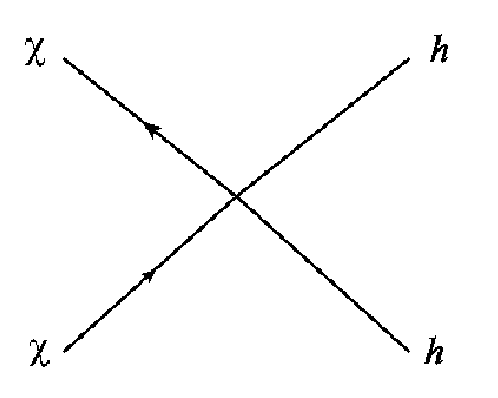


As a consequence of Eq. (36), and pairs may annihilate into a variety of standard model particles. The leading diagrams are shown in Fig. 6. The cross section for annihilations into fermions is given by
| (37) |
where is the number of fermion colors ( for leptons and for quarks) and is the fermion mass. The cross sections for annihilations into and bosons are given by
| (38) |
| (39) |
where () is the mass of () boson. In the case where the dark matter annihilates into a pair of standard model Higgs bosons, we can safely ignore the - and -channel diagrams since the typical momenta are much smaller than at temperatures near freeze out. Hence, the cross section is given by
| (40) |
The evolution of dark matter number density, , is governed by the Boltzmann equation
| (41) |
where is the Hubble parameter as a function of time and is the equilibrium number density. The thermally-averaged annihilation cross section, , can be calculated by evaluating the integral [33]
| (42) |
where is the total annihilation cross section and the are modified Bessel functions of order . We find the freeze out temperature, , using the freeze-out condition [34]
| (43) |
where equilibrium number density as a function of temperature is given by
| (44) |
The Hubble parameter may be re-expressed as a function of temperature
| (45) |
where is the number of relativistic degrees of freedom and GeV is the Planck mass. It is customary to normalize the temperature with the dark matter mass, . For the points in parameter space discussed below, we found that the freeze out happens when . The present dark matter density can be calculated using the relation
| (46) |
where is the ratio of number to entropy density and the subscript denotes the present time. The ratio of the dark matter relic density to the critical density is given by , where is the present entropy density, or equivalently
| (47) |
Note that the factor of included in the expression for takes into account the contribution from particles and antiparticles.
In the case TeV, we find numerically that the dark matter-Higgs coupling in order that . For TeV, we find . These order-one couplings are perturbative. One should keep in mind that the physics responsible for dark matter annihilations is not directly linked to the mechanism that we have proposed to account for dark matter decay; other contributions to the total annihilation cross section can easily be arranged. For example, if the Higgs sector includes mixing with a gauge singlet scalar such that there is a scalar mass eigenstate near , then the annihilation through the -channel exchange of this state can lead to a resonantly enhanced annihilation channel, as in the model of Ref. [8]. In this case, the correct relic density could be obtained for smaller than the values quoted above.
Finally, we confirm that the model does not conflict with bounds from searches for dark matter-nuclear recoil. In this case, the most relevant contribution comes from the interaction between the dark matter and quarks mediated by a -channel Higgs exchange. The effective Lagrangian is given by
| (48) |
Following Refs [35, 36], we can write an effective interaction between the nucleons and dark matter,
| (49) |
where , for or . The coefficient can be evaluated using the results of Ref. [36]; numerically, one finds with . Given the effective dark matter-nucleon interaction, we find that the spin-independent cross section is given by
| (50) |
For both of the cases discussed earlier, and , we find . This is two orders of magnitude smaller than the strongest bounds, from CDMS [37], which range from cm2 at TeV to cm2 at TeV.
V Conclusions
Models of decaying dark matter require a plausible origin for the higher-dimension operators that lead to dark matter decays. The data from cosmic ray experiments like PAMELA and Fermi-LAT require that these operators involve lepton fields preferentially. We have shown how the desired higher-dimension operators may originate from Planck-suppressed couplings between a TeV-scale scalar dark matter particle and vector-like states at a mass scale that is intermediate between the weak and Planck scales. The vector-like sector has the structure of a Froggatt-Nielsen model: charged lepton Yukawa couplings arise only after these states are integrated out and a discrete gauged Abelian flavor symmetry is broken. Couplings between and the standard model gauge-invariant combination are then also generated, with coefficients of order , where is the scale at which the flavor symmetry is broken. Taking and near the geometric mean of the reduced Planck scale and the weak scale, GeV, leads to the desired dark matter lifetime. Neutrino masses can be generated via a conventional see-saw mechanism with the mass scale of right-handed neutrinos also near . We pointed out that the symmetry structure of our model leads to an overall suppression factor multiplying the charged lepton Yukawa matrix, but does not constrain the standard model Yukawa textures otherwise. Hence, our framework is potentially compatible with a wide range of possible solutions to the more general problem of quark and lepton flavor in the standard model.
We presented the necessary PYTHIA simulations to confirm that our model can account for the anomalies observed in the cosmic ray experiments discussed earlier. The leading contribution to the primary cosmic ray electron and positron flux in our model comes from two-body decays, in which the Higgs field is set equal to its vev in the operator described above; the subleading three body decays, , are also possible. We have checked that these decay channels do not lead to an observable excess in the spectrum of cosmic ray antiprotons, since the cosmic ray antiproton flux is in agreement with astrophysical predictions.
Our model demonstrates that the desired lifetime and decay channels of TeV-scale scalar dark matter candidate can be the consequence of renormalizable physics at an intermediate lepton flavor scale and gravitational physics at . This presents an alternative scenario to the one in which dark matter decay is a consequence of physics at a unification scale located somewhere between and .
Acknowledgements.
We thank Josh Erlich and Marc Sher for useful comments. This work was supported by the NSF under Grant PHY-0757481. In addition, C.D.C. gratefully acknowledges support from a William & Mary Plumeri Fellowship.References
- [1] A. A. Abdo et al. [The Fermi LAT Collaboration], Phys. Rev. Lett. 102, 181101 (2009) [arXiv:0905.0025 [astro-ph.HE]].
- [2] F. Aharonian et al. [H.E.S.S. Collaboration], Astron. Astrophys. 508, 561 (2009) [arXiv:0905.0105 [astro-ph.HE]].
- [3] O. Adriani et al. [PAMELA Collaboration], Nature 458, 607 (2009) [arXiv:0810.4995 [astro-ph]].
- [4] W. Mitthumsiri, “Cosmic-Ray Positron Measurement with the Fermi-LAT Using the Earth’s Magnetic Field,” Talk presented at the 2011 Fermi Symposium, Rome, 9-12 May 2011, [http://fermi.gsfc.nasa.gov/science/symposium/2011/program/].
- [5] O. Adriani et al., Phys. Rev. Lett. 102, 051101 (2009) [arXiv:0810.4994 [astro-ph]].
- [6] D. Hooper, P. Blasi and P. D. Serpico, JCAP 0901, 025 (2009) [arXiv:0810.1527 [astro-ph]]; H. Yuksel, M. D. Kistler and T. Stanev, Phys. Rev. Lett. 103, 051101 (2009) [arXiv:0810.2784 [astro-ph]].
- [7] A. Ibarra and D. Tran, JCAP 0902 (2009) 021; E. Nardi, F. Sannino and A. Strumia, JCAP 0901 (2009) 043; R. Essig, N. Sehgal and L.E. Strigari, Phys. Rev. D 80 (2009) 023506; D. Malyshev, I. Cholis and J. Gelfand, Phys. Rev. D 80 (2009) 063005; V. Barger, Y. Gao, W.Y. Keung, D. Marfatia and G. Shaughnessy, Phys. Lett. B 678 (2009) 283; P. Meade, M. Papucci, A. Strumia and T. Volansky, Nucl. Phys. B 831 (2010) 178; L. Zhang, G. Sigl and J. Redondo, JCAP 0909 (2009) 012; A. Ibarra, D. Tran and C. Weniger, JCAP 1001, 009 (2010); M. Cirelli, P. Panci and P. D. Serpico, Nucl. Phys. B 840 (2010) 284; L. Covi, M. Grefe, A. Ibarra and D. Tran, JCAP 1004 (2010) 017; L. Zhang, C. Weniger, L. Maccione, J. Redondo and G. Sigl, JCAP 1006, 027 (2010); G. Hutsi, A. Hektor and M. Raidal, JCAP 1007 (2010) 008; J. Ke, M. Luo, L. Wang, G. Zhu, Phys. Lett. B698, 44-51 (2011); M. Garny, A. Ibarra, D. Tran, C. Weniger, JCAP 1101, 032 (2011); L. Dugger, T. E. Jeltema, S. Profumo, JCAP 1012, 015 (2010).
- [8] C. D. Carone, J. Erlich, R. Primulando, Phys. Rev. D82, 055028 (2010). [arXiv:1008.0642 [hep-ph]].
- [9] H. Fukuoka, J. Kubo, D. Suematsu, Phys. Lett. B678, 401-406 (2009). [arXiv:0905.2847 [hep-ph]].
- [10] A. Arvanitaki, S. Dimopoulos, S. Dubovsky, P. W. Graham, R. Harnik, S. Rajendran, Phys. Rev. D79, 105022 (2009). [arXiv:0812.2075 [hep-ph]]; Phys. Rev. D80, 055011 (2009). [arXiv:0904.2789 [hep-ph]].
- [11] H. S. Goh, L. J. Hall and P. Kumar, JHEP 0905 (2009) 097; C.R. Chen and F. Takahashi, JCAP 0902 (2009) 004; Y. Nomura and J. Thaler, Phys. Rev. D 79 (2009) 075008; P. f. Yin, Q. Yuan, J. Liu, J. Zhang, X.j. Bi and S.h. Zhu, Phys. Rev. D 79 (2009) 023512; K. Ishiwata, S. Matsumoto and T. Moroi, Phys. Lett. B 675 (2009) 446; C.R. Chen, M.M. Nojiri, F. Takahashi and T.T. Yanagida, Prog. Theor. Phys. 122 (2009) 553; X. Chen, JCAP 0909 (2009) 029; K. Ishiwata, S. Matsumoto and T. Moroi, JHEP 0905 (2009) 110; M. Endo and T. Shindou, JHEP 0909 (2009) 037; S.L. Chen, R.N. Mohapatra, S. Nussinov and Y. Zhang, Phys. Lett. B 677 (2009) 311; A. Ibarra, A. Ringwald, D. Tran and C. Weniger, JCAP 0908 (2009) 017; S. Shirai, F. Takahashi and T.T. Yanagida, Phys. Lett. B 680 (2009) 485; C.H. Chen, C.Q. Geng and D.V. Zhuridov, Eur. Phys. J. C 67 (2010) 479; J. Mardon, Y. Nomura and J. Thaler, Phys. Rev. D 80 (2009) 035013; K.Y. Choi, D.E. Lopez-Fogliani, C. Munoz and R.R. de Austri, JCAP 1003 (2010) 028; D. Aristizabal Sierra, D. Restrepo and O. Zapata, Phys. Rev. D 80 (2009) 055010; W.L. Guo, Y.L. Wu and Y.F. Zhou, Phys. Rev. D 81 (2010) 075014; X. Gao, Z. Kang, T. Li, Eur. Phys. J. C69, 467-480 (2010); S. Matsumoto, K. Yoshioka, Phys. Rev. D82, 053009 (2010); K. -Y. Choi, D. Restrepo, C. E. Yaguna, O. Zapata, JCAP 1010, 033 (2010); K. Ishiwata, S. Matsumoto, T. Moroi, JHEP 1012, 006 (2010); K. Hamaguchi, S. Shirai and T. T. Yanagida, Phys. Lett. B 673 (2009) 247; B. Kyae, JCAP 0907 (2009) 028; P.H. Frampton and P.Q. Hung, Phys. Lett. B 675 (2009) 411; M. Kadastik, K. Kannike and M. Raidal, Phys. Rev. D 81 (2010) 015002; Phys. Rev. D 80 (2009) 085020; Q. -H. Cao, E. Ma, G. Shaughnessy, Phys. Lett. B673, 152-155 (2009); J.H. Huh and J.E. Kim, Phys. Rev. D 80 (2009) 075012; M. Luo, L. Wang, W. Wu and G. Zhu, Phys. Lett. B 688 (2010) 216; C. Arina, T. Hambye, A. Ibarra and C. Weniger, JCAP 1003 (2010) 024; J. Schmidt, C. Weniger and T. T. Yanagida, arXiv:1008.0398; Y. Kajiyama, H. Okada, Nucl. Phys. B848, 303-313 (2011).
- [12] N. Haba, Y. Kajiyama, S. Matsumoto, H. Okada, K. Yoshioka, Phys. Lett. B695, 476-481 (2011). [arXiv:1008.4777 [hep-ph]].
- [13] C. D. Froggatt, H. B. Nielsen, Nucl. Phys. B147, 277 (1979).
- [14] T. Banks, M. Dine, Phys. Rev. D45, 1424-1427 (1992). [hep-th/9109045].
- [15] K. Nakamura et al. [ Particle Data Group Collaboration ], J. Phys. G G37, 075021 (2010).
- [16] A. Ibarra, D. Tran, C. Weniger, JCAP 1001, 009 (2010). [arXiv:0906.1571 [hep-ph]].
- [17] T. Delahaye, R. Lineros, F. Donato, N. Fornengo, P. Salati, Phys. Rev. D77, 063527 (2008). [arXiv:0712.2312 [astro-ph]]; F. Donato, N. Fornengo, D. Maurin, P. Salati, Phys. Rev. D69, 063501 (2004). [astro-ph/0306207].
- [18] T. Sjostrand, S. Mrenna, P. Z. Skands, Comput. Phys. Commun. 178, 852-867 (2008). [arXiv:0710.3820 [hep-ph]].
- [19] J. F. Navarro, C. S. Frenk, S. D. M. White, Astrophys. J. 462, 563-575 (1996). [astro-ph/9508025].
- [20] A. Ibarra, D. Tran, JCAP 0807, 002 (2008). [arXiv:0804.4596 [astro-ph]].
- [21] S. W. Barwick et al. [ HEAT Collaboration ], Astrophys. J. 482, L191-L194 (1997). [astro-ph/9703192].
- [22] M. Aguilar et al. [ AMS-01 Collaboration ], Phys. Lett. B646, 145-154 (2007). [astro-ph/0703154 [ASTRO-PH]].
- [23] M. Boezio et al. [ CAPRICE Collaboration ], Astrophys. J. 532, 653-669 (2000).
- [24] M. Ackermann et al. [ Fermi LAT Collaboration ], Phys. Rev. D82, 092004 (2010). [arXiv:1008.3999 [astro-ph.HE]].
- [25] F. Aharonian et al. [ H.E.S.S. Collaboration ], Phys. Rev. Lett. 101, 261104 (2008). [arXiv:0811.3894 [astro-ph]]; F. Aharonian et al. [ H.E.S.S. Collaboration ], Astron. Astrophys. 508, 561 (2009). [arXiv:0905.0105 [astro-ph.HE]].
- [26] S. Torii et al. [ PPB-BETS Collaboration ], [arXiv:0809.0760 [astro-ph]].
- [27] M. A. DuVernois, S. W. Barwick, J. J. Beatty, A. Bhattacharyya, C. R. Bower, C. J. Chaput, S. Coutu, G. A. de Nolfo et al., Astrophys. J. 559, 296-303 (2001).
- [28] V. S. Ptuskin, I. V. Moskalenko, F. C. Jones, A. W. Strong, V. N. Zirakashvili, Astrophys. J. 642, 902-916 (2006). [astro-ph/0510335].
- [29] O. Adriani et al. [ PAMELA Collaboration ], Phys. Rev. Lett. 105, 121101 (2010). [arXiv:1007.0821 [astro-ph.HE]].
- [30] M. Boezio et al. [ WIZARD Collaboration ], Astrophys. J. 487, 415-423 (1997); M. Boezio et al. [ WiZard/CAPRICE Collaboration ], Astrophys. J. 561, 787-799 (2001). [astro-ph/0103513].
- [31] S. Orito et al. [ BESS Collaboration ], Phys. Rev. Lett. 84, 1078-1081 (2000). [astro-ph/9906426].
- [32] J. W. Mitchell, L. M. Barbier, E. R. Christian, J. F. Krizmanic, K. Krombel, J. F. Ormes, R. E. Streitmatter, A. W. Labrador et al., Phys. Rev. Lett. 76, 3057-3060 (1996).
- [33] P. Gondolo, G. Gelmini, Nucl. Phys. B360, 145-179 (1991).
- [34] E. W. Kolb and M. S. Turner, “The Early Universe,” Boulder, Colorado: Westview Press (1994) 547p.
- [35] J. McDonald, Phys. Rev. D50, 3637-3649 (1994). [hep-ph/0702143 [HEP-PH]].
- [36] J. R. Ellis, A. Ferstl, K. A. Olive, Phys. Lett. B481, 304-314 (2000). [hep-ph/0001005].
- [37] Z. Ahmed et al. [ The CDMS-II Collaboration ], Science 327, 1619-1621 (2010). [arXiv:0912.3592 [astro-ph.CO]].