On Stochastic Gradient and Subgradient Methods
with Adaptive Steplength Sequences

Farzad Yousefian Angelia Nedić Uday V. Shanbhag ^†^†thanks: The authors are with the Department of Industrial and Enterprise Systems Engineering, University of Illinois, Urbana, IL 61801, USA, {yousefi1,angelia,udaybag}@illinois.edu. Nedić and Shanbhag gratefully acknowledge the support of the NSF through the award NSF CMMI 0948905 ARRA.

Abstract

Traditionally, stochastic approximation (SA) schemes have been popular choices for solving stochastic optimization problems. However, the performance of standard SA implementations can vary significantly based on the choice of the steplength sequence, and in general, little guidance is provided about good choices. Motivated by this gap, in the first part of the paper, we present two adaptive steplength schemes for strongly convex differentiable stochastic optimization problems, equipped with convergence theory, that aim to overcome some of the reliance on user-specific parameters. Of these, the first scheme, referred to as a recursive steplength stochastic approximation (RSA) scheme, optimizes the error bounds to derive a rule that expresses the steplength at a given iteration as a simple function of the steplength at the previous iteration and certain problem parameters. The second scheme, termed as a cascading steplength stochastic approximation (CSA) scheme, maintains the steplength sequence as a piecewise-constant decreasing function with the reduction in the steplength occurring when a suitable error threshold is met.

In the second part of the paper, we allow for nondifferentiable objectives but with bounded subgradients over a certain domain. In such a regime, we propose a local smoothing technique, based on random local perturbations of the objective function, that leads to a differentiable approximation of the function. Assuming a uniform distribution on the local randomness, we establish a Lipschitzian property for the gradient of the approximation and prove that the obtained Lipschitz bound grows at a modest rate with problem size. This facilitates the development of an adaptive steplength stochastic approximation framework, which now requires sampling in the product space of the original measure and the artificially introduced distribution. The resulting adaptive steplength schemes are applied to three stochastic optimization problems. In particular, we observe that both schemes perform well in practice and display markedly less reliance on user-defined parameters.

I Introduction

The use of stochastic gradient and subgradient schemes for the solution of stochastic convex optimization problems has a long tradition, beginning with an iterative scheme, first proposed by Robbins and Monro [1], that relied primarily on noisy gradient observations. Research by Ermoliev and his coauthors [2, 3, 4, 5] focused largely on quasigradient (subgradient) methods and considered a host of stochastic programming problems, amongst them being two-period recourse-based problems (see [6]). To accelerate the convergence of stochastic subgradient methods, ergodic sequences, arising from the averaging of iterates, have been employed in [7, 8, 9, 10]. Often gradient computations are either costly or unavailable; in such instances, a finite-difference approximation of the gradient can be constructed as first observed by Kiefer and Wolfowitz [11]. While standard finite-difference techniques perturb one direction at a time to obtain gradient estimates, simultaneous perturbation stochastic approximation techniques simultaneously perturb all directions and general require fewer function evaluations [12, 13]. More recently, there has been a significant interest in the application of ODE-based methods for investigating the stability and convergence of the associated stochastic approximation schemes [14, 15]. An elegant exposition of these methods may be found in the monographs by Polyak [16], Kushner and Yin [17], and Borkar [15].

Sample-average approximation (SAA) techniques [18] are often viewed as an alternative to stochastic approximation techniques and are particularly attractive when approximate solutions to the problem are desired in an offline manner. This approach relies on using a sample from the underlying distribution to construct a deterministic sample-average problem, which can be subsequently solved via standard nonlinear programming solvers, as seen in [19]. In [10], the authors demonstrate that stochastic approximation schemes are shown to be competitive with SAA techniques. Importantly in [10], Nemirovski et al. develop a robust SA scheme that determines an optimal constant steplength for minimizing the theoretical error over a pre-specified number of steps. Mirror-descent generalizations of SA, that rely on a suitably defined prox-mapping, are also presented in [10] (also see [20]), while validation analysis is provided in [21].

Stochastic gradient algorithms have also been found to be effective in solving large deterministic problems such as convex feasibility problems [9, 22, 23], feasibility problems arising in control [24, 25] and some specially structured large-scale convex problems in [26, 27, 28]. Distributed consensus-based stochastic subgradient methods for minimizing a convex objective over a network have been recently developed and studied in [29, 30, 31]. The success of gradient-based methods in solving monotone variational inequalities [32] has prompted the study of similar techniques for contending with stochastic variational inequalities. In fact, Jiang and Xu [33] develop precisely such a scheme for the solution of strongly monotone stochastic variational inequalities and regularized variants were presented in [34] to allow for application to monotone stochastic variational inequalities. Finally, stochastic generalizations of the mirror-prox schemes were examined in [35] and allowed for the solution of monotone variational inequalities.

While stochastic approximation schemes have proved successful, other avenues exist for addressing stochastic programs. For instance, an alternate approach lies in using sample-average approximation methods, that obtain estimators to the optimal value and solution of the problem through the solution of deterministic problem in which the expectation is replaced by a sample-average. Convergence theory for the obtained estimators is examined by Shapiro [18]. Decomposition schemes, that leverage cutting-plane methods, have also been particularly successful in addressing two-period stochastic linear [36], convex [37] and nonconvex programs [38] while a scalable matrix-splitting decomposition scheme is presented in [39] for two-period stochastic Nash games.

In this paper, we consider adaptive stochastic gradient and subgradient methods for solving constrained stochastic convex optimization problems. The novelty of our work can be categorized as follows: (1) the development and analysis of two adaptive stepsize rules; and (2) the development of a local function smoothing technique. Next, we provide some motivation and a more elaborate description of each.

In stochastic gradient methods (cf. [2, 3, 4, 5, 16, 40, 14, 17, 15]), the almost-sure convergence of such methods is guaranteed assuming that the stepsize is diminishing but not too rapidly, i.e., the stepsize is proportional to $\frac{1}{k^{a}}$ with $\frac{1}{2}<a\leq 1$ . Typically, there is no guidance on the specific choice of the sequence and problem parameters play little role in refining this choice. In contrast, in this paper, we propose specific (adaptive) rules for the stepsize values that exploit the information about the objective function. Accordingly, our first goal lies in examining whether one can construct a convergent scheme under an adaptive stepsize rule that is more reflective of the problem setting. Through out this part of the paper, we assume that the integrand of the expectation is a random convex differentiable function. Under a Lipschitzian assumption on the gradient, we propose two different adaptive stepsize rules:

(a)

Recursive stepsize rule: In attempting to minimize the bound on the expected error, we develop a recursive scheme for specifying the stepsize that requires only the steplength at the previous parameter and some problem parameters. Global convergence and rate estimates for this scheme are developed.
(b)

Cascading stepsize rule: It is well-known that under suitable assumptions, fixed-stepsize schemes are guaranteed to converge to a compact region containing the solution set of the original problem. We consider a modified version of such a scheme where the trajectory moves to successively smaller compact regions containing the solution sets. Furthermore, as soon as the trajectory of iterates reaches within a bound of the solution set, the steplength is updated allowing the sequence to make further progress. Effectively, we consider a method in which the steplength sequence can be viewed as one where the stepsize is maintained constant with drops or cascades in stepsize occurring at particular epochs. While the scheme has intuitive appeal, we provide a theoretical support for the convergence of such an algorithmic framework.

When the random integrands arising in such stochastic problems are nonsmooth, direct application of known SA schemes is impossible. Contending with nonsmoothness in mathematical programming is often managed through avenues that rely on the solution of a sequence of smoothed problems (cf. [41, 42]). In a stochastic regime, an approach for addressing such problems is through a technique of global smoothing, as considered in [43] and more recently in [44].¹¹ 1 See [45] for a scheme that develops an approximation method for addressing a class of separable piecewise-linear stochastic optimization problems with integer breakpoints. This involves modifying the original problem by adding a random variable with possibly unbounded support. However, such a technique is not feasible in when the objective is defined over a restricted domain. We present a local smoothing technique which leads to a globally differentiable approximation of the original function with Lipschitz continuous gradients. Furthermore, through such a smoothing, we derive a Lipschitz constant for the gradients and show that the constant grows at the rate of $\sqrt{n}$ where $n$ is the dimensionality of the problem space. Importantly, this Lipschitzian property facilitates the construction of a stochastic approximation framework. Consequently, the second part of the paper focuses on computing solutions to approximations with smoothed integrands whose gradients are shown to be provably Lipschitz continuous.

The remainder of the paper is organized as follows. In Section II, we establish the almost-sure convergence of the classical stochastic approximation algorithm for a constrained problem with a differentiable convex function with Lipschitz gradients. In Sections III and IV, for a strongly convex function, we propose and analyze two different stepsize rules, each motivated by a minimization of an estimate on the expected error per iteration of the method. In Section V, we introduce a local randomized smoothing technique for nondifferentiable convex optimization, and derive its approximation properties as well as a bound on the Lipschitz constant of the gradients. In Section VI, we report some numerical results obtained by applying our proposed stepsize rules and the smoothing technique to three test problems and conclude with a discussion in Section VII.

Notation and basic terminology: We view vectors as columns, and write $x^{T}$ to denote the transpose of a vector $x$ . We use $\|x\|$ to denote the Euclidean vector norm, i.e., $\|x\|=\sqrt{x^{T}x}$ . We write $\Pi_{X}(x)$ to denote the Euclidean projection of a vector $x$ on a set $X$ . i.e., $\|x-\Pi_{X}(x)\|=\min_{y\in X}\|x-y\|$ . For a convex function $f$ with domain ${\rm dom}f$ , a vector $g$ is a subgradient of $f$ at $\bar{x}\in{\rm dom}f$ if the following relation holds²² 2 For a differentiable convex $f$ , the inequality holds with $g=\nabla f(\bar{x})$ .:

f(\bar{x})+g^{T}(x-\bar{x})\leq f(x)\qquad\hbox{for all $x\in{\rm dom}f$}.

The subdifferential set of $f$ at $x=\bar{x}$ , denoted by $\partial f(\bar{x})$ , is the set of all subgradients of $f$ at $x=\bar{x}$ . Finally, we write a.s. for “almost surely”, and use $\hbox{Prob}(\mathcal{Z})$ and $\mathsf{E}\!\left[Z\right]$ to denote the probability of an event $\mathcal{Z}$ and the expectation of a random variable $Z$ , respectively.

II Problem Formulation and Background

In this section, we begin by describing the problem and iterative scheme of interest (Section II-A). This is followed by Section II-B where we provide a short description on various adaptive schemes in the realm of stochastic approximation.

II-A Problem Formulation

We consider the following stochastic optimization problem

\min_{x\in X}f(x)=\mathsf{E}\!\left[F(x,\xi)\right],

(1)

where $F:\mathcal{D}\times\Omega\to\mathbb{R}$ is a function, the set $\mathcal{D}\subseteq\mathbb{R}^{n}$ is open, and the set $X$ is nonempty with $X\subset\mathcal{D}$ . The vector $\xi:\Omega\rightarrow\mathbb{R}^{d}$ is a random vector with a probability distribution on a set $\Omega\subseteq\mathbb{R}^{d}$ , while the expectation $\mathsf{E}\!\left[F(x,\xi)\right]$ is taken with respect to $\xi$ . We use $X^{*}$ to denote the optimal set of problem (1) and $f^{*}$ to denote its optimal value. We assume the following:

Assumption 1

The set $X\subset\mathcal{D}$ is convex and closed. The function $F(\cdot,\xi)$ is convex on $\mathcal{D}$ for every $\xi\in\Omega$ , and the expected value $\mathsf{E}\!\left[F(x,\xi)\right]$ is finite for every $x\in\mathcal{D}$ .

Under Assumption 1, the function $f$ is convex over $X$ and the following relation holds

\partial{f(x)}=\mathsf{E}\!\left[\partial_{x}F(x,\xi)\right]\qquad\hbox{for all }x\in\mathcal{D},

(2)

where $\partial_{x}F(x,\xi)$ denotes the set of all subgradients of $F(x,\xi)$ with respect to the variable $x$ (see [46, 47]³³ 3 In both of these articles, the analysis is for a function defined over $\mathbb{R}^{n}\times\Omega$ , but can be extended to the case of a function defined over $\mathcal{D}\times\Omega$ for an open convex set $\mathcal{D}\subseteq\mathbb{R}^{n}$ .).

First, we will consider problem (1) where $f$ is a differentiable function with Lipschitz gradients. Later, we will allow the function $f$ to be nondifferentiable and we will consider a local smoothing technique yielding a differentiable function that approximates $f$ over $X$ . For this reason, we start our discussion by focusing on a differentiable problem (1) and the following iterative algorithm:

\begin{split}x_{k+1}&=\Pi_{X}\left(x_{k}-\gamma_{k}(\nabla f(x_{k})+w_{k})\right)\qquad\hbox{for all }k\geq 0,\cr w_{k}&=\nabla_{x}F(x_{k},\xi_{k})-\nabla f(x_{k}).\end{split}

(3)

Here, $x_{0}\in X$ is a random initial point, $\gamma_{k}>0$ is a (deterministic) stepsize, and $w_{k}$ is the random vector given by the difference between the sampled gradient $\nabla_{x}F(x,\xi_{k})$ and its expectation $\mathsf{E}\!\left[\nabla_{x}F(x,\xi)\right]$ evaluated at $x=x_{k}$ . Throughout the paper, we assume that $\mathsf{E}\!\left[\|x_{0}\|^{2}\right]<\infty$ .

We let $\mathcal{F}_{k}$ denote the history of the method up to time $k$ , i.e., $\mathcal{F}_{k}=\{x_{0},\xi_{0},\xi_{1},\ldots,\xi_{k-1}\}$ for $k\geq 1$ and $\mathcal{F}_{0}=\{x_{0}\}$ . By Assumption 1 and relation (2), it follows that $\nabla f(x_{k})=\mathsf{E}\!\left[\nabla_{x}F(x_{k},\xi)\right]$ for a differentiable $F$ , implying that $w_{k}$ has zero-mean, i.e.,

\mathsf{E}\!\left[w_{k}\mid\mathcal{F}_{k}\right]=0\qquad\hbox{for all }k\geq 0.

(4)

Next, we state some additional assumptions on the stochastic gradient error $w_{k}$ and the stepsize $\gamma_{k}$ .

Assumption 2

The stepsize is such that $\gamma_{k}>0$ for all $k$ . Furthermore, the following hold:

(a)

$\sum_{k=0}^{\infty}\gamma_{k}=\infty$ and $\sum_{k=0}^{\infty}\gamma_{k}^{2}<\infty$ .
(b)

The stochastic errors $w_{k}$ satisfy $\sum_{k=0}^{\infty}\gamma_{k}^{2}\mathsf{E}\!\left[\|w_{k}\|^{2}\mid\mathcal{F}_{k}\right]<\infty$ almost surely.

Assumption 2(b) is satisfied, for example, when $\sum_{k=0}^{\infty}\gamma_{k}^{2}<\infty$ and the error $w_{k}$ is bounded almost surely, i.e., $\|w_{k}\|\leq c$ for all $k$ and some scalar $c$ almost surely.

We use the following Lemma in establishing the convergence of method (3) (see [16], page 50).

Lemma 1

(Robbins-Siegmund) Let $v_{k},$ $u_{k},$ $\alpha_{k},$ and $\beta_{k}$ be nonnegative random variables, and let the following relations hold almost surely:

\mathsf{E}\!\left[v_{k+1}\mid{\tilde{\mathcal{F}}_{k}}\right]\leq(1+\alpha_{k})v_{k}-u_{k}+\beta_{k}\quad\hbox{ for all }k,\qquad\sum_{k=0}^{\infty}\alpha_{k}<\infty,\qquad\sum_{k=0}^{\infty}\beta_{k}<\infty,

where $\tilde{\mathcal{F}}_{k}$ denotes the collection $v_{0},\ldots,v_{k}$ , $u_{0},\ldots,u_{k}$ , $\alpha_{0},\ldots,\alpha_{k}$ , $\beta_{0},\ldots,\beta_{k}$ . Then, almost surely we have

\lim_{k\to\infty}v_{k}=v,\qquad\sum_{k=0}^{\infty}u_{k}<\infty,

where $v\geq 0$ is some random variable.

We also make use of the following result, which can be found in [16] (see Lemma 11 in page 50).

Lemma 2

Let $\{v_{k}\}$ be a sequence of nonnegative random variables, where $\mathsf{E}\!\left[v_{0}\right]<\infty$ , and let $\{\alpha_{k}\}$ and $\{\beta_{k}\}$ be deterministic scalar sequences such that:

		$\displaystyle\mathsf{E}\!\left[v_{k+1}\|v_{0},\ldots,v_{k}\right]\leq(1-\alpha_{k})v_{k}+\beta_{k}\qquad a.s\ \hbox{for all }k\geq 0,$
		$\displaystyle 0\leq\alpha_{k}\leq 1,\quad\ \beta_{k}\geq 0,\quad\ \sum_{k=0}^{\infty}\alpha_{k}=\infty,\quad\ \sum_{k=0}^{\infty}\beta_{k}<\infty,\quad\ \lim_{k\to\infty}\,\frac{\beta_{k}}{\alpha_{k}}=0.$

Then, $v_{k}\rightarrow 0$ almost surely, $\lim_{k\to\infty}\mathsf{E}\!\left[v_{k}\right]=0$ , and for any $\epsilon>0$ ,

\hbox{Prob}(v_{j}\leq\epsilon\hbox{ for all }j\geq k)\geq 1-\frac{1}{\epsilon}\left(\mathsf{E}\!\left[v_{k}\right]+\sum_{i=k}^{\infty}\beta_{i}\right)\qquad\hbox{for all $k>0$}.

In Sections III and IV, we examine adaptive steplength schemes for a strongly convex function $f$ whose gradients $\nabla f$ are Lipschitz continuous over $X$ with constant $L$ . $X$ is defined as

II-B Adaptive Stochastic Approximation Schemes

Robbins and Monro [1] proposed the first stochastic approximation algorithm in 1951 while Kiefer and Wolfowitz [11] proposed a variant of this scheme in which finite differences were employed to estimate the gradient. Asymptotic distributions of the Robbins-Monro scheme were first examined by Chung [48], leading to an asymptotic normality result in the one-dimensional regime while generalizations were subsequently studied by Sacks [49].

A potential challenge in developing efficient implementations of stochastic approximation implementations lies in choosing an appropriate steplength sequence. Kesten [50], in 1957, suggested a technique where the steplength sequence adapts to the observed data, which was further extended by Kushner and Gavin [51] to the multi-dimensional regime, while its accelerations were studied in [52]. Sacks [49] proved that, under suitable conditions, a choice of the form $a/k$ (where $k$ is the iterate index) is optimal from the standpoint of minimizing the asymptotic variance. Yet, the challenge lies in estimating the “optimal” $a$ . Subsequently, Ventner [53] in what is possibly amongst the first adaptive steplength SA schemes, considered sequences of the form $a_{k}/k$ where $a_{k}$ is updated by leveraging past information. Notably, Chung [48] also examined the asymptotic variance properties of SA when steplength choices of the form $a/k^{1-\alpha}$ with $\alpha<{1\over 2}$ are used. In related work on adaptive schemes, Lai and Robbins [54] considered schemes of the form $a_{k}/k$ where $a_{k}$ is a strongly consistent estimator of $\nabla f(x)$ in a stochastic root-finding problem. One choice for obtaining $a_{k}$ is through the use of least-squares estimators. Multivariate generalizations of this analysis were suggested by Wei [55] in 1987 and again, it was observed that the Jacobian of the vector function assumes relevance in constructing efficient steplength sequences.

An alternative to using a single sample was suggested by Spall [12] and relied on obtaining gradient estimates through a simultaneous perturbation of all the parameters. An adaptive generalization of this scheme, proposed by the same author [56, 57], employed an additional recursion to the standard projected gradient step that attempted to estimate the Jacobian in root finding problems or the Hessian in optimization problems. Accordingly, the modified update rule is of the form

x_{k+1}=\Pi_{X}\left(x_{k}-\gamma_{k}H_{k}^{-1}(\nabla f(x_{k})+w_{k})\right),

(5)

where $H_{k}$ is an estimate of the Hessian matrix of the objective. Clearly, this also falls under the regime of an adaptive steplength scheme. Related adaptive schemes may also be found in the work by Bhatnagar [58, 59].

A final remark is in order regarding the key difference between our proposed schemes and past work. A majority of the adaptive schemes in the literature employ past information to update the steplength. One such avenue involves developing estimates of the Hessian which is subsequently used in scaling the gradient step appropriately. In the sections to appear, we consider two very different approaches that are linked by a crucial property: they rely on using algorithm and problem parameters, and not sample points, to develop adaptive steplength schemes.

II-C Smoothing Techniques

One of the goals of this paper is to address stochastic optimization problems with nonsmooth integrands. Here, we provide some background for accommodating nonsmoothness in optimization problems. In deterministic regimes, subgradient methods and their incremental variants have proved popular (see [26, 27, 60]), as have bundle methods [61], amongst others. One approach for managing nonsmoothness is through smoothing approaches. For instance, such avenues have allowed for the solution of variational inequalities and complementarity problems [32] as well as mathematical programs with equilibrium constraints [62].

In this paper, we also adopt a smoothing technique which bears little similarity to such approaches. We adopt a framework that can be traced back to a class of averaged functions introduced by Steklov [63, 64] in 1907. A general definition of such an averaging over possibly discontinuous functions is provided next [65].

Definition 1

Given a locally integrable function $f:\mathbb{R}^{n}\to\mathbb{R}$ and a family of mollifiers $\{p_{\epsilon}:\mathbb{R}^{n}\to\mathbb{R}_{+},\epsilon>0\}$ that satisfy

\int_{\mathbb{R}^{n}}p_{\epsilon}(z)dz=1,\qquad\textrm{supp}(p_{\epsilon}):=\{z\in\mathbb{R}^{n}:p_{\epsilon}(z)>0\}\subset\rho_{\epsilon}\mathbb{B}\mbox{ with }\rho_{\epsilon}\downarrow 0\hbox{ as }\epsilon\downarrow 0,

where $\mathbb{B}$ is a unit ball in $\mathbb{R}^{n}$ . Then the associated family $\{\hat{f}_{\epsilon},\epsilon>0\}$ of averaged functions is defined by

\hat{f}_{\epsilon}:=\int_{\mathbb{R}^{n}}f(x+z)p_{\epsilon}(z)dz=\int_{\mathbb{R}^{n}}f(z)p_{\epsilon}(x-z)dz.

In effect, the mollifier is a probability density function and the family of smoothed approximations, denoted by $\{\hat{f}_{\epsilon},\epsilon>0\}$ must possess a host of convergence properties with respect to $f$ as $\epsilon\to 0$ . For instance, if $f$ is a continuous function then $\hat{f}_{\epsilon}$ converges uniformly to $f$ on every bounded subset of $\mathbb{R}^{n}$ . In the absence of continuity, this cannot be guaranteed; yet, we may draw on epi-convergence results [66] for this class of functions may be employed in an effort to establish convergence of the infima/minima. These averaging functions have allowed for solving convex nondifferentiable optimization problems [67, 68] and discontinuous optimization problems [69], by minimizing a sequence of averaged or smoothed functions.

We pursue an alternative to solving a sequence of smoothed problems and obtain an approximate solution by solving a single smoothed problem with a fixed $\epsilon$ akin to that employed by Lakshmanan and Farias [44]. However, since we intend to leverage stochastic approximation schemes of the form described earlier in this paper, Lipschitz constants associated with the gradients are a requiem. In [44], the authors obtain Lipschitz constants assuming that the averaging is achieved through a normal distribution that requires the function be defined everywhere. Instead of “globally smoothing” the function, we employ a uniform distribution, referred to as “local smoothing.”

III A recursive steplength stochastic approximation scheme

In this section, we introduce an adaptive stochastic approximation scheme that overcomes certain challenges associated with implementing standard diminishing steplength schemes and relies on the use of a recursive rule for prescribing steplengths. We begin by examining the standard stochastic gradient method for problem (1) in Section III-A. In general, the convergence of this scheme is guaranteed under the requirement that $\sum_{k=1}^{\infty}\gamma_{k}=\infty$ and $\sum_{k=0}^{\infty}\gamma_{k}^{2}<\infty.$ A host of choices exists with one possible choice being $\gamma_{k}=\theta/k.$ Yet, the choice of the appropriate $\theta$ can have a significant impact on the performance of the algorithm. Motivated by the desire to minimize the “expected error,” we develop a recursive stochastic approximation algorithm (referred to as the RSA scheme) in which the steplength at a particular iteration is a function of the steplength at the previous iteration and some problem parameters. In Section III-B, we motivate and introduce such a scheme and proceed to develop the associated convergence theory in Section III-C.

III-A Preliminaries

We consider method (3) as applied to problem (1) where $f$ has Lipschitz gradients. The method generates a sequence of iterates that converge to an optimal solution almost-surely, as shown in the forthcoming proposition. This result is a straightforward extension of Theorem 1 in [16, Pg. 51] which pertains to an unconstrained problem.

Proposition 1 (Almost-sure convergence)

Let Assumptions 1–2 hold, and let $f$ be differentiable over the set $X$ with Lipschitz gradients. Assume that the optimal set $X^{*}$ of problem (1) is nonempty. Then, the sequence $\{x_{k}\}$ generated by (3) converges almost surely to some random point in $X^{*}$ .

Proof:

By definition of the method and the nonexpansive property of the projection operation, we obtain for any $x^{*}\in X^{*}$ and $k\geq 0$ ,

	$\displaystyle\\|x_{k+1}-x^{*}\\|^{2}$	$\displaystyle\leq\\|x_{k}-x^{*}-\gamma_{k}(\nabla f(x_{k})+w_{k})\\|^{2}$
		$\displaystyle=\\|x_{k}-x^{}\\|^{2}-2\gamma_{k}(\nabla f(x_{k})+w_{k})^{T}(x_{k}-x^{})+\gamma_{k}^{2}\\|\nabla f(x_{k})+w_{k}\\|^{2}.$

By the convexity of $f$ and the gradient inequality, we have

\displaystyle\|x_{k+1}-x^{*}\|^{2}

\displaystyle\leq\|x_{k}-x^{*}\|^{2}-2\gamma_{k}(f(x_{k})-f(x^{*}))-2\gamma_{k}w_{k}^{T}(x_{k}-x^{*})+\gamma_{k}^{2}\|\nabla f(x_{k})+w_{k}\|^{2}.

Since $\|a+b\|^{2}\leq 2\|a\|^{2}+2\|b\|^{2}$ for any $a,b\in\mathbb{R}^{n}$ , by using $f^{*}=f(x^{*})$ , and by adding and subtracting $\nabla f(x^{*})$ in the last term, we obtain

	$\displaystyle\\|x_{k+1}-x^{*}\\|^{2}$	$\displaystyle\leq\\|x_{k}-x^{}\\|^{2}-2\gamma_{k}(f(x_{k})-f^{})-2\gamma_{k}w_{k}^{T}(x_{k}-x^{})+2\gamma_{k}^{2}\\|\nabla f(x_{k})-\nabla f(x^{})\\|^{2}$
		$\displaystyle+2\gamma_{k}^{2}\\|\nabla f(x^{*})+w_{k}\\|^{2}.$

Taking the conditional expectation given $\mathcal{F}_{k}$ , using $\mathsf{E}\!\left[w_{k}\mid\mathcal{F}_{k}\right]=0$ (see Eq. (4)) and the Lipschitzian property of the gradient, we have

	$\displaystyle\mathsf{E}\!\left[\\|x_{k+1}-x^{*}\\|^{2}\mid\mathcal{F}_{k}\right]$	$\displaystyle\leq(1+2L^{2}\gamma_{k}^{2})\\|x_{k}-x^{}\\|^{2}-2\gamma_{k}(f(x_{k})-f^{})$
		$\displaystyle+2\gamma_{k}^{2}\left(\\|\nabla f(x^{*})\\|^{2}+\mathsf{E}\!\left[\\|w_{k}\\|^{2}\mid\mathcal{F}_{k}\right]\right).$

Under Assumption 2, the conditions of Lemma 1 are satisfied. Therefore, almost surely, the sequence $\{\|x_{k+1}-x^{*}\|\}$ is convergent for any $x^{*}\in X^{*}$ and $\sum_{k=0}^{\infty}\gamma_{k}(f(x_{k})-f^{*})<\infty$ . The former relation implies that $\{x_{k}\}$ is bounded a.s., while the latter implies $\liminf_{k\to\infty}f(x_{k})=f^{*}$ a.s. in view of the condition $\sum_{k=0}^{\infty}\gamma_{k}=\infty$ . Since the set $X$ is closed, all accumulation points of $\{x_{k}\}$ lie in $X$ . Furthermore, since $f(x_{k})\to f^{*}$ along a subsequence a.s., by continuity of $f$ it follows that $\{x_{k}\}$ has a subsequence converging to some random point in $X^{*}$ a.s. Moreover, since $\{\|x_{k+1}-x^{*}\|\}$ is convergent for any $x^{*}\in X^{*}$ a.s., the entire sequence $\{x_{k}\}$ converges to some random point in $X^{*}$ a.s. ∎

Under the Lipschitz continuity of the gradient and the strong convexity of the objective, an expected error bound may also be provided for the method. During the development of the error bound, the following intermediate result assumes relevance.

Lemma 3

Let Assumption 1 hold, and let $f$ be differentiable over the set $X$ with Lipschitz gradients with constant $L>0$ . Also, assume that the optimal set $X^{*}$ of problem (1) is nonempty. Let the sequence $\{x_{k}\}$ be generated by algorithm (3) with any (deterministic) stepsize $\gamma_{k}>0$ . Then, for any $x^{*}\in X^{*}$ and any $k\geq 0$ , the following holds almost surely:

\displaystyle\mathsf{E}\!\left[\|x_{k+1}-x^{*}\|^{2}\mid\mathcal{F}_{k}\right]\leq\|x_{k}-x^{*}\|^{2}+\gamma_{k}^{2}\mathsf{E}\!\left[\|w_{k}\|^{2}\mid\mathcal{F}_{k}\right]-\gamma_{k}(2-\gamma_{k}L)(x_{k}-x^{*})^{T}(\nabla f(x_{k})-\nabla f(x^{*})).

Proof:

By the first-order optimality conditions, a vector $x^{*}$ is optimal for the problem if and only if $x^{*}$ satisfies

x^{*}=\Pi_{X}(x^{*}-\gamma\nabla f(x^{*}))\qquad\hbox{for any }\gamma>0.

By the definition of the method and the nonexpansive property of the projection operation, we obtain for all $k\geq 0$ ,

\begin{split}\|x_{k+1}-x^{*}\|^{2}&=\|\Pi_{X}(x_{k}-\gamma_{k}(\nabla f(x_{k})+w_{k}))-\Pi_{X}(x^{*}-\gamma_{k}\nabla f(x^{*}))\|^{2}\\ &\leq\|x_{k}-x^{*}-\gamma_{k}(\nabla f(x_{k})+w_{k}-\nabla f(x^{*}))\|^{2}.\end{split}

Taking the expectation conditioned on the past, and using $\mathsf{E}\!\left[w_{k}\mid\mathcal{F}_{k}\right]=0$ (cf. Eq. (4)), we have

\begin{split}\mathsf{E}\!\left[\|x_{k+1}-x^{*}\|^{2}\mid\mathcal{F}_{k}\right]&\leq\|x_{k}-x^{*}\|^{2}+\gamma_{k}^{2}\|\nabla f(x_{k})-\nabla f(x^{*})\|^{2}+\gamma_{k}^{2}\mathsf{E}\!\left[\|w_{k}\|^{2}\mid\mathcal{F}_{k}\right]\cr&-2\gamma_{k}(x_{k}-x^{*})^{T}(\nabla f(x_{k})-\nabla f(x^{*})).\end{split}

The Lipschitz gradient property for a convex function is equivalent to co-coercivity of the gradient map with constant $1/L$ , (see [16, Pg. 24, Lemma 2]), i.e., for all $x,y\in X$ ,

\frac{1}{L}\,\|\nabla f(x)-\nabla f(y)\|^{2}\leq(x-y)^{T}(\nabla f(x)-\nabla f(y)).

Therefore, for any $x^{*}\in X^{*}$ and any $k\geq 0$ ,

\mathsf{E}\!\left[\|x_{k+1}-x^{*}\|^{2}\mid\mathcal{F}_{k}\right]\leq\|x_{k}-x^{*}\|^{2}+\gamma_{k}^{2}\mathsf{E}\!\left[\|w_{k}\|^{2}\mid\mathcal{F}_{k}\right]-\gamma_{k}(2-\gamma_{k}L)(x_{k}-x^{*})^{T}(\nabla f(x_{k})-\nabla f(x^{*})).

∎

In what follows, we will often use a stronger version of Assumption 2(b), given as follows.

Assumption 3

The errors $w_{k}$ are such that for some $\nu>0$ ,

\mathsf{E}\!\left[\|w_{k}\|^{2}|\mathcal{F}_{k}\right]\leq\nu^{2}\quad a.s.\ \hbox{for all $k\geq 0$}.

Next, we provide an error bound for algorithm (3) under the assumption that $f(x)$ is a strongly convex function with Lipschitz gradients. Note that requiring that $f(x)$ is strongly convex over a set $K$ follows if $F(x,\xi(\omega))$ is a strongly convex function for $\omega\in\bar{\Omega}$ , where $\bar{\Omega}$ is a set of positive measure defined as

\bar{\Omega}\triangleq\left\{\omega:\exists\eta>0,(y-x)^{T}(\nabla F(y,\xi(\omega))-\nabla F(x,\xi(\omega)))\geq\eta\|x-y\|^{2}\quad\hbox{for all }x,y\in K\right\}.

Less formally, we merely require that $F(.,\xi)$ is a strongly convex function with positive, but arbitrarily small, probability to ensure that $f(x)$ is strongly convex over $K$ (see [70]).

Lemma 4 (Strongly convex function with Lipschitz gradients)

Let Assumptions 1–2 hold. Also, let $f$ be differentiable over the set $X$ with Lipschitz gradients with constant $L>0$ and strongly convex with constant $\eta>0$ . Then, the sequence $\{x_{k}\}$ generated by algorithm (3) converges almost surely to the unique optimal solution of problem (1). Furthermore, if the stepsize satisfies $0<\gamma_{k}\leq\frac{2}{L}$ for all $k\geq 0$ , we then have:

(a)

The following relation holds almost surely:

\mathsf{E}\!\left[\|x_{k+1}-x^{*}\|^{2}\mid\mathcal{F}_{k}\right]\leq\left(1-\gamma_{k}(2-\gamma_{k}L)\right)\|x_{k}-x^{*}\|^{2}+\gamma_{k}^{2}\mathsf{E}\!\left[\|w_{k}\|^{2}\mid\mathcal{F}_{k}\right]\qquad\hbox{for all }k\geq 0.

(b)

If Assumption 2(b) is replaced with Assumption 3, then the following relation holds almost surely:

\mathsf{E}\!\left[\|x_{k+1}-x^{*}\|^{2}\right]\leq(1-\eta\gamma_{k}(2-\gamma_{k}L))\mathsf{E}\!\left[\|x_{k}-x^{*}\|^{2}\right]+\gamma_{k}^{2}\nu^{2}\quad\hbox{for all }k\geq 0.

Moreover, $\lim_{k\to\infty}\mathsf{E}\!\left[\|x_{k}-x^{*}\|^{2}\right]=0$ , and for every $\epsilon>0$ ,

\hbox{Prob}\left(\|x_{j}-x^{*}\|^{2}\leq\epsilon\hbox{ for all }j\geq k\right)\geq 1-\frac{1}{\epsilon}\,\left(\mathsf{E}\!\left[\|x_{k}-x^{*}\|^{2}\right]+\nu^{2}\sum_{i=k}^{\infty}\gamma_{i}^{2}\right)\qquad\hbox{for all $k>0$}.

Proof:

The existence and uniqueness of the optimal solution of problem (1) is guaranteed by the strong convexity of $f(x)$ . The convergence of the method follows by Proposition 1. To establish the relation in part (a) for the expected value $\mathsf{E}\!\left[\|x_{k+1}-x^{*}\|^{2}\right]$ , we use Lemma 3, which implies for the optimal $x^{*}$ and all $k\geq 0$ ,

\displaystyle\mathsf{E}\!\left[\|x_{k+1}-x^{*}\|^{2}\mid\mathcal{F}_{k}\right]\leq\|x_{k}-x^{*}\|^{2}+\gamma_{k}^{2}\mathsf{E}\!\left[\|w_{k}\|^{2}\mid\mathcal{F}_{k}\right]-\gamma_{k}(2-\gamma_{k}L)(x_{k}-x^{*})^{T}(\nabla f(x_{k})-\nabla f(x^{*})).

By the strong convexity of $f(x)$ , we have $(x-y)^{T}(\nabla f(x)-\nabla f(y))\geq\eta\|x-y\|^{2}$ for all $x,y\in X$ , which when combined with the preceding relation implies for all $k\geq 0$ ,

\displaystyle\mathsf{E}\!\left[\|x_{k+1}-x^{*}\|^{2}\mid\mathcal{F}_{k}\right]\leq\left(1-\gamma_{k}\eta(2-\gamma_{k}L)\right)\|x_{k}-x^{*}\|^{2}+\gamma_{k}^{2}\mathsf{E}\!\left[\|w_{k}\|^{2}\mid\mathcal{F}_{k}\right],

(6)

thus showing the relation in part (a).

The relation in part (b), follows from inequality (6) by using Assumption 3 and by taking the total expectation. To show the other results in part (b), we apply Lemma 2. For this, we need to verify that all the conditions of Lemma 2 hold. Since $0<\gamma_{k}\leq\frac{2}{L}$ , it follows $\eta\gamma_{k}(2-\gamma_{k}L)\geq 0$ . Also, in view of $\eta\leq L$ , we have $\eta\gamma_{k}(2-\gamma_{k}L)\leq 1$ . Obviously, $\nu^{2}\gamma_{k}^{2}\geq 0$ for all $k$ . Since Assumption 2(a) holds, we have $\sum_{k=0}^{\infty}\eta\gamma_{k}(2-\gamma_{k}L)=\infty$ and $\sum_{k=0}^{\infty}\eta\gamma_{k}^{2}<\infty$ . Furthermore, since $\gamma_{k}\to 0$ , we have

\lim_{k\to\infty}\frac{\nu^{2}\gamma_{k}^{2}}{\eta\gamma_{k}(2-\gamma_{k}L)}=\lim_{k\to\infty}\frac{\nu^{2}\gamma_{k}}{\eta(2-\gamma_{k}L)}=0.

Hence, the conditions of Lemma 2 hold and the stated results follow. ∎

Lemma 4 will be employed in developing our adaptive stepsize schemes. Before proceeding, we make the following comment regarding the lemma.

Remark 1: The result in part (a) of Lemma 4 is similar to a result in [10], which was derived by requiring only the strong convexity of the function $f$ . Here, we make the additional assumption that the gradients are Lipschitz continuous and this assumption gains relevance when we employ local random smoothing in Section V. Furthermore, our result depends on the expectation of gradient errors, $\mathsf{E}\!\left[\|w_{k}\|^{2}\right]$ , with $w_{k}$ defined in (3). Note that, in contrast, the result in [10] depends on the expectation of the subgradient norms, $\mathsf{E}\!\left[\|G(x,\xi)\|^{2}\right]$ , where $G(x,\xi)\in\partial_{x}F(x,\xi)$ .

III-B A recursive steplength scheme

A challenge associated with the implementation of diminishing steplength schemes lies in determining an appropriate sequence $\{\gamma_{k}\}$ . The key result of this section is the motivation and introduction of a scheme that adaptively optimizes the steplength from iteration to iteration. Our adaptive scheme relies on the minimization of a suitably defined error function at each step. We start with the relation in part (b) of Lemma 4:

\mathsf{E}\!\left[\|x_{k+1}-x^{*}\|^{2}\right]\leq(1-\eta\gamma_{k}(2-\gamma_{k}L))\mathsf{E}\!\left[\|x_{k}-x^{*}\|^{2}\right]+\gamma_{k}^{2}\nu^{2}\quad\hbox{for all }k\geq 0.

(7)

When the stepsize is further restricted so that $0<\gamma_{k}\leq\frac{1}{L}$ , we have

1-\eta\gamma_{k}(2-\gamma_{k}L)\leq 1-\eta\gamma_{k}.

Thus, for $0<\gamma_{k}\leq\frac{1}{L}$ , inequality (7) yields

\mathsf{E}\!\left[\|x_{k+1}-x^{*}\|^{2}\right]\leq(1-\eta\gamma_{k})\mathsf{E}\!\left[\|x_{k}-x^{*}\|^{2}\right]+\gamma_{k}^{2}\nu^{2}\qquad\hbox{for all }k\geq 0.

(8)

We now use relation (8) to develop an adaptive stepsize procedure. Loosely speaking for the moment, let us view the quantity $\mathsf{E}\!\left[\|x_{k+1}-x^{*}\|^{2}\right]$ as an error $e_{k+1}$ of the method arising from the use of the stepsize values $\gamma_{0},\gamma_{1},\ldots,\gamma_{k}$ . Also, consider the worst case error which is the case when (8) holds with equality. Thus, in the worst case, the error satisfies the following recursive relation:

e_{k+1}(\gamma_{0},\ldots,\gamma_{k})=(1-\eta\gamma_{k})e_{k}(\gamma_{0},\ldots,\gamma_{k-1})+\gamma_{k}^{2}\nu^{2}.

Then, it seems natural to investigate if the stepsizes $\gamma_{0},\gamma_{1}\ldots,\gamma_{k}$ can be selected so as to minimize the error $e_{k+1}$ . It turns out that this can indeed be achieved and minimizing the error $e_{k+2}$ at the next iteration can also be done by selecting $\gamma_{k+1}$ as a function of only the most recent stepsize $\gamma_{k}$ . To formalize the above discussion, we define real-valued error functions $e_{k}(\gamma_{0},\ldots,\gamma_{k-1})$ as follows:

\displaystyle e_{k}(\gamma_{0},\ldots,\gamma_{k-1})

\displaystyle\triangleq(1-\eta\gamma_{k-1})e_{k-1}(\gamma_{0},\ldots,\gamma_{k-2})+\gamma_{k-1}^{2}\nu^{2}\qquad\hbox{for $k\geq 1$},

(9)

where $e_{0}$ is a positive scalar, $\eta$ is the strong convexity parameter and $\nu^{2}$ is the upper bound for the second moments of the error norms $\|w_{k}\|$ .

In what follows, we consider the sequence $\{\gamma^{*}_{k}\}$ given by

		$\displaystyle\gamma_{0}^{*}=\frac{\eta}{2\nu^{2}}\,e_{0}$		(10)
		$\displaystyle\gamma_{k}^{}=\gamma_{k-1}^{}\left(1-\frac{\eta}{2}\gamma_{k-1}^{*}\right)\quad\hbox{for all }k\geq 1.$		(11)

We often abbreviate $e_{k}(\gamma_{0},\ldots,\gamma_{k-1})$ by $e_{k}$ whenever this is unambiguous. We show that the stepsizes $\gamma_{i}$ , $i=0,\ldots,k-1,$ minimize the errors $e_{k}$ over an $(0,\frac{1}{L}]^{k}$ , where $L$ is the Lipschitz constant. In particular, we have the following result.

Proposition 2

Let $e_{k}(\gamma_{0},\ldots,\gamma_{k-1})$ be defined as in (9), where $e_{0}>0$ is such that $\frac{\eta}{2\nu^{2}}\,e_{0}\leq\frac{1}{L}$ , with $L$ being the Lipschitz constant for the gradients of $f$ . Let the sequence $\{\gamma^{*}_{k}\}$ be given by (10)–(11). Then, the following hold:

(a)

The error $e_{k}$ satisfies

$\displaystyle e_{k}(\gamma_{0}^{*},\ldots,\gamma_{k-1}^{*})=\frac{2\nu^{2}}{\eta}\,\gamma_{k}^{*}\qquad\hbox{for all $k\geq 0$}.$

(b)

For each $k\geq 1$ , the vector $(\gamma_{0}^{*},\gamma_{1}^{*},\ldots,\gamma_{k-1}^{*})$ is the minimizer of the function $e_{k}(\gamma_{0},\ldots,\gamma_{k-1})$ over the set

\mathbb{G}_{k}\triangleq\left\{\alpha\in\mathbb{R}^{k}:0<\alpha_{j}\leq\frac{1}{L}\hbox{ for }j=1,\ldots,k\right\}.

More precisely, for any $k\geq 1$ and any $(\gamma_{0},\ldots,\gamma_{k-1})\in\mathbb{G}_{k}$ , we have

\displaystyle e_{k}(\gamma_{0},\ldots,\gamma_{k-1})-e_{k}(\gamma_{0}^{*},\ldots,\gamma_{k-1}^{*})\geq\nu^{2}(\gamma_{k-1}-\gamma_{k-1}^{*})^{2}.

(c)

The vector $\gamma^{*}=(\gamma_{0}^{*},\gamma_{1}^{*},\ldots,\gamma_{k-1}^{*})$ is a stationary point of function $e_{k}(\gamma_{0},\gamma_{1},\ldots,\gamma_{k-1})$ over the set $\mathbb{G}_{k}$ .

Proof:

(a) We use induction on $k$ to prove our result. Note that the result holds trivially for $k=0$ from (10). Next, assume that we have $e_{k}(\gamma_{0}^{*},\ldots,\gamma_{k-1}^{*})=\frac{2\nu^{2}}{\eta}\,\gamma_{k}^{*}$ for some $k$ , and consider the case for $k+1$ . By the definition of the error $e_{k}$ in (9), we have

e_{k+1}(\gamma_{0}^{*},\ldots,\gamma_{k}^{*})=(1-\eta\gamma^{*}_{k})e_{k}(\gamma^{*}_{0},\ldots,\gamma_{k-1}^{*})+\gamma_{k}^{*}\nu^{2}=(1-\eta\gamma^{*}_{k})\frac{2\nu^{2}}{\eta}\,\gamma_{k}^{*}+\gamma_{k}^{*}\nu^{2},

where the second equality follows by the inductive hypothesis. Hence,

e_{k+1}(\gamma_{0}^{*},\ldots,\gamma_{k}^{*})=\frac{2\nu^{2}}{\eta}\,\gamma_{k}^{*}\left(1-\eta\gamma^{*}_{k}+\frac{\eta}{2}\,\gamma^{*}_{k}\right)=\frac{2\nu^{2}}{\eta}\,\gamma_{k}^{*}\left(1-\frac{\eta}{2}\,\gamma^{*}_{k}\right)=\frac{2\nu^{2}}{\eta}\,\gamma_{k+1}^{*},

where the last equality follows by the definition of $\gamma^{*}_{k+1}$ in (11).

(b) We now show that $(\gamma^{*}_{0},\gamma_{1}^{*},\ldots,\gamma_{k-1}^{*})$ minimizes the error $e_{k}$ for all $k\geq 1$ . We again use mathematical induction on $k$ . By the definition of the error $e_{1}$ and the relation $e_{1}(\gamma_{0}^{*})=\frac{2\nu^{2}}{\eta}\gamma_{1}^{*}$ shown in part (a), we have

e_{1}(\gamma_{0})-e_{1}(\gamma_{0}^{*})=(1-\eta\gamma_{0})e_{0}+\nu^{2}\gamma_{0}^{2}-\frac{2\nu^{2}}{\eta}\gamma_{1}^{*}.

Using $\gamma_{1}^{*}=\gamma_{0}^{*}\left(1-\frac{\eta}{2}\gamma_{0}^{*}\right)$ , we obtain

e_{1}(\gamma_{0})-e_{1}(\gamma_{0}^{*})=(1-\eta\gamma_{0})e_{0}+\nu^{2}\gamma_{0}^{2}-\frac{2\nu^{2}}{\eta}\gamma_{0}^{*}\left(1-\frac{\eta}{2}\gamma_{0}^{*}\right)=(1-\eta\gamma_{0})\frac{2\nu^{2}}{\eta}\,\gamma_{0}^{*}+\nu^{2}\gamma_{0}^{2}-\frac{2\nu^{2}}{\eta}\gamma_{0}^{*}\left(1-\frac{\eta}{2}\gamma_{0}^{*}\right),

where the last equality follows from $e_{0}=\frac{2\nu^{2}}{\eta}\,\gamma_{0}^{*}.$ Thus, we have

e_{1}(\gamma_{0})-e_{1}(\gamma_{0}^{*})=-2\nu^{2}\gamma_{0}\gamma_{0}^{*}+\nu^{2}\gamma_{0}^{2}+\nu^{2}\,(\gamma_{0}^{*})^{2}=\nu^{2}\left(\gamma_{0}-\gamma_{0}^{*}\right)^{2}.

Now suppose that $e_{k}(\gamma_{0},\ldots,\gamma_{k-1})\geq e_{k}(\gamma_{0}^{*},\ldots,\gamma_{k-1}^{*})$ holds for some $k$ and any $(\gamma_{0},\ldots,\gamma_{k-1})\in\mathbb{G}_{k}$ . We want to show that $e_{k+1}(\gamma_{0},\ldots,\gamma_{k})\geq e_{k+1}(\gamma_{0}^{*},\ldots,\gamma_{k}^{*})$ holds as well for all $(\gamma_{0},\ldots,\gamma_{k})\in\mathbb{G}_{k+1}$ . To simplify the notation we use $e_{k+1}^{*}$ to denote the error $e_{k+1}$ evaluated at $(\gamma^{*}_{0},\gamma_{1}^{*},\ldots,\gamma_{k}^{*})$ , and $e_{k+1}$ when evaluating at an arbitrary vector $(\gamma_{0},\gamma_{1},\ldots,\gamma_{k})\in\mathbb{G}_{k+1}$ . Using (9) and part (a), we have

\displaystyle e_{k+1}-e_{k+1}^{*}=(1-\eta\gamma_{k})e_{k}+\nu^{2}\gamma_{k}^{2}-\frac{2\nu^{2}}{\eta}\gamma_{k+1}^{*}.

Under the inductive hypothesis, we have $e_{k}\geq e_{k}^{*}$ . Using this, the relation $e_{k}^{*}=\frac{2\nu^{2}}{\eta}\gamma_{k}^{*}$ of part (a) and the definition of $\gamma_{k+1}^{*}$ , we obtain

\displaystyle e_{k+1}-e_{k+1}^{*}\geq(1-\eta\gamma_{k})\frac{2\nu^{2}}{\eta}\gamma_{k}^{*}+\nu^{2}\gamma_{k}^{2}-\frac{2\nu^{2}}{\eta}\gamma_{k}^{*}\left(1-\frac{\eta}{2}\gamma_{k}^{*}\right)=\nu^{2}(\gamma_{k}-\gamma_{k}^{*})^{2}.

Hence, we have $e_{k}(\gamma_{0},\ldots,\gamma_{k-1})-e_{k}(\gamma^{*}_{0},\ldots,\gamma_{k-1}^{*})\geq\nu^{2}(\gamma_{k}-\gamma_{k}^{*})^{2}$ for all $k\geq 1$ and all $(\gamma_{0},\ldots,\gamma_{k-1})\in\mathbb{G}_{k}$ . Therefore, for all $k\geq 1$ , the vector $(\gamma_{0},\ldots,\gamma_{k-1})\in\mathbb{G}_{k}$ is a minimizer of the error $e_{k}$ .

(c) By the choice of $e_{0}$ , we have $0<\gamma_{0}^{*}<\frac{1}{L}$ . Observe that since $\eta\leq L$ , it follows that $0<\gamma^{*}_{1}\leq\gamma^{*}_{0}$ , and by induction we can see that $0<\gamma^{*}_{k}\leq\gamma^{*}_{k-1}$ for all $k\geq 1$ . Thus, $(\gamma^{*}_{0},\ldots,\gamma_{k-1}^{*})\in\mathbb{G}_{k}$ for all $k\geq 1$ .

Now, we proceed by induction on $k$ . For $k=1$ , we have

\frac{\partial e_{1}}{\partial\gamma_{0}}=-\eta e_{0}+2\gamma_{0}\nu^{2}.

Thus, the derivative of $e_{1}$ vanishes at $\gamma_{0}^{*}=\frac{\eta}{2\nu}\,e_{0}$ , which satisfies $0<\gamma_{0}^{*}\leq\frac{1}{L}$ by the choice of $e_{0}$ . Furthermore, note that the function $e_{1}(\gamma_{0})$ is convex in $\gamma_{0}$ . Hence, $\gamma_{0}^{*}=\frac{\eta}{2\nu}\,e_{0}$ is the stationary point of $e_{1}$ over the entire real line. Suppose now that for $k\geq 1$ , the vector $(\gamma_{0},\ldots,\gamma_{k-1})$ is the minimizer of $e_{k}$ over the set $G_{k}$ . Let us now consider the case of $k+1$ . The partial derivative of $e_{k+1}$ with respect to $\gamma_{\ell}$ is given by

\displaystyle\frac{\partial e_{k+1}}{\partial\gamma_{\ell}}

\displaystyle=-\eta e_{0}\prod_{i=0,i\neq\ell}^{k}(1-\eta\gamma_{i})-\eta\nu^{2}\sum_{i=0}^{\ell-1}\left(\gamma_{i}^{2}\prod_{j=i+1,j\neq\ell}^{k}(1-\eta\gamma_{j})\right)+2\nu^{2}\gamma_{\ell}\prod_{i=\ell+1}^{k}(1-\eta\gamma_{i}),

where $0\leq\ell\leq k-1.$ By factoring out the common term $\prod_{i=\ell+1}^{k}(1-\eta\gamma_{i})$ , we obtain

\displaystyle\frac{\partial e_{k+1}}{\partial\gamma_{\ell}}=\left[-\eta\left(e_{0}\prod_{i=0}^{\ell-1}(1-\eta\gamma_{i})+\nu^{2}\sum_{i=0}^{\ell-2}\left(\gamma_{i}^{2}\prod_{j=i+1}^{\ell-1}(1-\eta\gamma_{j})\right)+\nu^{2}\gamma_{\ell-1}^{2}\right)+2\nu^{2}\gamma_{\ell}\right]\prod_{i=\ell+1}^{k}(1-\eta\gamma_{i}).

(12)

From the definition of $e_{k}$ in (9) we can see that

\displaystyle e_{k+1}(\gamma_{0},\ldots,\gamma_{k})=e_{0}\prod_{i=0}^{k}(1-\eta\gamma_{i})+\nu^{2}\sum_{i=0}^{k-1}\left(\gamma_{i}^{2}\prod_{j=i+1}^{k}(1-\eta\gamma_{j})\right)+\nu^{2}\gamma_{k}^{2}.

(13)

By combining relations (12) and (13), we obtain for all $\ell=0,\ldots,k-1,$

\frac{\partial e_{k+1}}{\partial\gamma_{\ell}}=\left(-\eta e_{\ell}(\gamma_{0},\ldots,\gamma_{\ell-1}\right)+2\nu^{2}\gamma_{\ell})\prod_{i=\ell+1}^{k}(1-\eta\gamma_{i}),

where for $\ell=0$ , we have $e_{\ell}(\gamma_{0},\ldots,\gamma_{\ell-1})=e_{0}$ . By part (a), there holds $-\eta e_{\ell}(\gamma_{0}^{*},\ldots,\gamma_{\ell-1}^{*})+2\nu^{2}\gamma_{\ell}^{*}=0$ , thus showing that $\frac{\partial e_{k+1}}{\partial\gamma_{\ell}}$ vanishes at $(\gamma^{*}_{0},\ldots,\gamma_{k}^{*})\in\mathbb{G}_{k+1}$ for all $\ell=0,\ldots,k-1$ .

Finally, we consider the partial derivative of $e_{k+1}$ with respect to $\gamma_{k}$ , for which we have

\displaystyle\frac{\partial e_{k+1}}{\partial\gamma_{k}}

\displaystyle=-\eta e_{0}\prod_{i=0}^{k-1}(1-\eta\gamma_{i})-\eta\nu^{2}\sum_{i=0}^{k-2}\left(\gamma_{i}^{2}\prod_{j=i+1}^{k-1}(1-\eta\gamma_{j})\right)-\eta\nu^{2}\gamma_{k-1}^{2}+2\nu^{2}\gamma_{k}.

Using relation (13), we obtain

\frac{\partial e_{k+1}}{\partial\gamma_{k}}=-\eta e_{k}(\gamma_{0},\ldots,\gamma_{k-1})+2\nu^{2}\gamma_{k}.

By part (a), we have $-\eta e_{k}(\gamma_{0}^{*},\ldots,\gamma_{k-1}^{*})+2\nu^{2}\gamma_{k}^{*}=0$ , thus showing that $\frac{\partial e_{k+1}}{\partial\gamma_{k}}$ vanishes at $(\gamma^{*}_{0},\ldots,\gamma_{k}^{*})\in\mathbb{G}_{k+1}$ . Thus, by induction we have that $(\gamma^{*}_{0},\ldots,\gamma_{k}^{*})$ is a stationary point of $e_{k+1}$ in the set $\mathbb{G}_{k+1}$ . ∎

We observe that in Proposition 2, the minimizer $(\gamma_{0}^{*},\ldots,\gamma_{k-1}^{*})$ of the function $e_{k}$ over the set $\mathbb{G}_{k}$ is unique up to scaling by a factor $\beta<1$ . Specifically, the solution $(\gamma_{0}^{*},\ldots,\gamma_{k-1}^{*})$ is obtained for an initial error $e_{0}>0$ satisfying $e_{0}<\frac{2\nu^{2}}{\eta L}.$ Suppose that in the definition of the sequence $\{\gamma_{k}^{*}\}$ instead of $e_{0}$ we use $\beta e_{0}$ for some $\beta\in(0,1)$ . Then it can be seen (by following the proof) that, for the resulting sequence, Proposition 2 would still hold.

III-C Convergence theory

We next show that the proposed RSA approximation scheme discussed in Section III-B leads to a convergent algorithm. We prove this in a more general setting for a stepsize with a form similar to that seen in constructing the optimal choice. The following proposition holds for any stepsize of a form similar to the optimal scheme of (11).

Proposition 3 (Global convergence of RSA scheme)

Let Assumptions 1 and 3 hold. Let the function $f$ be differentiable over the set $X$ with Lipschitz gradients and the optimal solution set of problem (1) be nonempty. Assume that the stepsize sequence $\{\gamma_{k}\}$ is generated by the following self-adaptive scheme:

\displaystyle\gamma_{k}=\gamma_{k-1}(1-c\gamma_{k-1})\qquad\hbox{for all }k\geq 1,

(14)

where $c>0$ is a scalar and the initial stepsize is such that $0<\gamma_{0}<\frac{1}{c}$ . Then, the sequence $\{x_{k}\}$ generated by algorithm (3) converges almost surely to a random point that belongs to the optimal set.

Proof:

We employ Proposition 1. To apply this proposition, it suffices to verify that Assumption 2 holds. First we show that $\sum_{i=0}^{\infty}{\gamma_{i}}=\infty$ . From (14) we obtain

\prod_{\ell=1}^{k+1}\gamma_{\ell}=\left(\prod_{i=0}^{k}\gamma_{i}\right)\prod_{i=0}^{k}(1-c\gamma_{i}).

By dividing both sides by $\left(\prod_{i=1}^{k}\gamma_{i}\right)$ , it follows that

\displaystyle\gamma_{k+1}=\gamma_{0}\prod_{i=0}^{k}(1-c\gamma_{i}).

(15)

Since $\gamma_{0}\in(0,\frac{1}{c})$ , from (14) it follows that $\{\gamma_{k}\}$ is positive nonincreasing sequence. Therefore, the limit $\lim_{k\to\infty}\gamma_{k}$ exists and it is less than $\frac{1}{c}$ . Thus, by taking the limit in (14), we obtain $\lim_{k\to\infty}\gamma_{k}=0$ . Then, by taking limits in (15), we further obtain

\lim_{k\rightarrow\infty}\prod_{i=0}^{k}(1-c\gamma_{i})=0.

To arrive at a contradiction suppose that $\sum_{i=0}^{\infty}{\gamma_{i}}<\infty$ . Then, there is an $\epsilon\in(0,1)$ such that for $j$ sufficiently large, we have

c\sum_{i=j}^{k}\gamma_{i}\leq\epsilon\quad\hbox{for all }k\geq j.

Since $\prod_{i=j}^{k}(1-c\gamma_{i})\geq 1-c\sum_{i=j}^{k}\gamma_{i}$ for all $j<k$ , by letting $k\rightarrow\infty$ , we obtain for all $j$ sufficiently large,

\prod_{i=j}^{\infty}(1-c\gamma_{i})\geq 1-c\sum_{i=j}^{\infty}\gamma_{i}\geq 1-\epsilon>0.

This, however, contradicts the fact $\lim_{k\rightarrow\infty}\prod_{i=0}^{k}(1-c\gamma_{i})=0.$ Therefore, we conclude that $\sum_{i=0}^{\infty}{\gamma_{i}}=\infty$ .

Now we show that $\sum_{i=0}^{\infty}{\gamma_{i}}^{2}<\infty$ . From (14) we have

\displaystyle\gamma_{k}=\gamma_{k-1}-c\gamma_{k-1}^{2}\quad\hbox{ for all }k\geq 1.

Summing the preceding relations, we obtain

\displaystyle\gamma_{k}=\gamma_{0}-c\sum_{i=0}^{k-1}{\gamma_{i}}^{2}\quad\hbox{ for all }k\geq 1.

By taking limits and recalling that $\lim_{k\to\infty}\gamma_{k}=0$ , we obtain

\displaystyle\sum_{i=0}^{\infty}{\gamma_{i}}^{2}=\frac{\gamma_{0}}{c}<\infty.

Assumption 3 and relation $\sum_{i=0}^{\infty}{\gamma_{i}}^{2}<\infty$ yield $\sum_{k=0}^{\infty}\gamma_{k}^{2}\mathsf{E}\!\left[\|w_{k}\|^{2}\mid\mathcal{F}_{k}\right]<\infty$ . Hence, Assumption 2 holds. ∎

Note that Proposition 3 applies to algorithm (3) with the stepsize sequence $\{\gamma_{k}^{*}\}$ generated by the recursive scheme (11). Thus, we immediately have the following corollary.

Corollary 1 (Convergence of RSA scheme)

Let Assumptions 1 and 3 hold. Let the function $f$ be differentiable over the set $X$ with Lipschitz gradients with constant $L>0$ and strongly convex with parameter $\eta>0$ . Let the stepsize sequence $\{\gamma_{k}^{*}\}$ be generated by the recursive scheme (11) with $e_{0}=\mathsf{E}\!\left[\|x_{0}-x^{*}\|^{2}\right]$ . If $\frac{\eta}{2\nu^{2}}\mathsf{E}\!\left[\|x_{0}-x^{*}\|^{2}\right]<\frac{1}{L},$ then the sequence $\{x_{k}\}$ generated by algorithm (3) converges almost surely to the unique optimal solution $x^{*}$ of problem (1).

Proof:

The existence and uniqueness of the optimal solution follows by the strong convexity assumption. Almost sure convergence follows by Proposition 3. ∎

Note that when the set $X$ is bounded, in Proposition 1 we may use $e_{0}=\max_{x,y\in X}\|x-y\|^{2}$ and the results will hold as long as $\frac{\eta}{2\nu^{2}}\max_{x,y\in X}\|x-y\|^{2}<\frac{1}{L}.$

In the following, we discuss a recursive stepsize for algorithm (3) as applied to a nonsmooth but strongly convex function $f(x)=\mathsf{E}\!\left[F(x,\xi)\right]$ . Let $G(x,\xi)$ be a subgradient vector of $F(x,\xi)$ with respect to $x$ , i.e., $G(x,\xi)\in\partial F(x,\xi)$ . Assume that there is a positive number $M$ such that

\mathsf{E}\!\left[\|G(x,\xi)\|^{2}\right]\leq M^{2}\quad\hbox{for all }x\in X.

We have the following convergence result, which obviously also holds for smooth problems.

Proposition 4 (Convergence of RSA with a nonsmooth objective)

Consider problem (1) and let Assumption 1 hold. Also, let the set $X$ be compact and the function $f$ be strongly convex over $X$ with constant $\eta$ . Assume that there is a scalar $M>0$ such that $\mathsf{E}\!\left[\|G(x,\xi)\|^{2}\right]\leq M^{2}$ for all $x\in X$ . Consider the following algorithm:

\begin{split}x_{k+1}&=\Pi_{X}\left(x_{k}-\gamma_{k}G(x_{k},\xi_{k})\right),\end{split}

(16)

where $x_{0}\in X$ is a random initial point independent of $\{\xi_{k}\}$ and $\gamma_{k}$ is a (deterministic) stepsize. Consider the self-adaptive stepsize sequence $\{\gamma_{k}^{*}\}$ defined by

		$\displaystyle\gamma_{0}^{*}=\frac{\eta}{M^{2}}D^{2},$
		$\displaystyle\gamma_{k}^{}=\gamma_{k-1}^{}(1-\eta\gamma_{k-1}^{*})\qquad\hbox{for all }k\geq 1,$

where $D=\max_{x,y\in X}\|x-y\|$ . Assuming that $\frac{\eta D^{2}}{M^{2}}<\frac{1}{2}$ , we have

\displaystyle\mathsf{E}\!\left[\|x_{k}-x^{*}\|^{2}\right]\leq\frac{M^{2}}{\eta}\gamma_{k}^{*}\qquad\hbox{for all }k\geq 1.

Proof:

The proof is based on verifying that, for the algorithm in (16), Proposition 2 holds, where $2\nu^{2}$ is replaced by $M^{2}$ and $e_{0}=D^{2}$ . Then, the rest of the proof is similar to that of Proposition 1. ∎

IV A cascading steplength stochastic approximation scheme

In Section III, we presented a stochastic approximation scheme in which the sequence of steplengths is determined via a recursion that relies on optimizing the error estimates. A key benefit of such a recursion is that the steplength choice is not left to the user. In this section, we introduce an alternate avenue for specifying steplengths that also considers a diminishing steplength framework but uses a markedly different approach for determining the steplength. In particular, the scheme relies on reducing the steplength at a set of epochs while the steplengths are maintained as constant between these epochs. The details of this stochastic approximation scheme (called the cascading steplength stochastic approximation (CSA) scheme) are presented in Section IV-A while convergence theory is provided in Section IV-B.

IV-A A cascading steplength scheme

Our technique is based on the properties derived from problems possessing strongly convex objectives. Specifically, we obtain the following result from the inequality in Lemma 4 when the stepsize is maintained as constant.

Proposition 5

Let Assumptions 1 and 3 hold. Also, let $f$ be differentiable over the set $X$ with Lipschitz gradients with constant $L>0$ and strongly convex with constant $\eta>0$ . Let the sequence $\{x_{k}\}$ be generated by (3) with constant stepsize $\gamma_{k}=\gamma$ for all $k\geq 0$ , where $\gamma\in(0,\frac{2}{L})$ . Then, we have

\mathsf{E}\!\left[\|x_{k}-x^{*}\|^{2}\right]\leq q(\gamma)^{k}\mathsf{E}\!\left[\|x_{0}-x^{*}\|^{2}\right]+\left(\frac{1-q(\gamma)^{k}}{1-q(\gamma)}\right)\gamma^{2}\nu^{2},

(17)

where $q(\gamma)=1-\eta\gamma(2-\gamma L)$ and $x^{*}$ is the optimal solution of problem (1).

Proof:

Follows from the inequality in part (b) of Lemma 4. ∎

From inequality (17), we obtain the following relation

\mathsf{E}\!\left[\|x_{k}-x^{*}\|^{2}\right]\leq\underbrace{q(\gamma)^{k}\mathsf{E}\!\left[\|x_{0}-x^{*}\|^{2}\right]}_{\rm Transient\,error}+\underbrace{\frac{\gamma^{2}\nu^{2}}{1-q(\gamma)}}_{\rm Persistent\,error}\quad\hbox{for all }k\geq 1,

(18)

where the expected distance $\mathsf{E}\!\left[\|x_{k}-x^{*}\|^{2}\right]$ is bounded by the sum of two error terms:

(1)

Transient error: The transient error, given by $q(\gamma)^{k}\mathsf{E}\!\left[\|x_{0}-x^{*}\|^{2}\right]$ , decays to zero as $k\to\infty.$ In effect, the contractive nature of this error, as arising from $q(\gamma)<1$ , ensures that the transient error can be reduced to an arbitrarily small level.
(2)

Persistent error: The persistent error, given by ${\frac{\gamma^{2}\nu^{2}}{1-q(\gamma)}}$ , is invariant to increasing the number of iterations, denoted by $k$ . Its reduction, as we proceed to show, necessitates reducing $\gamma.$

Our cascading steplength scheme basically requires specifying a rule for deciding at what iteration to decrease the steplength and to what extent it should be decreased. The iterations during which the stepsize is kept fixed is referred to as a constant steplength regime or just a regime. Given the two error terms, our scheme can be loosely represented as an infinite sequence of regimes of finite duration. In fact, we proceed to show that the duration of the regimes is an increasing function. Entering a new regime is marked by a reduction in the steplength. In fact, since a finite reduction in the steplength occurs between consecutive regimes, the steplength sequence would naturally converge to zero if there is an infinite number of the regimes. Suppose one is at the beginning of the $t$ th regime, where the steplength is $\gamma_{t}$ and the current iteration number is $K$ . The steplength $\gamma_{t}$ is maintained constant during regime $t$ . Furthermore, suppose that at the beginning of the $t$ th regime, the transient error is greater than the persistent error for $\gamma_{t}$ , i.e., $\mathsf{E}\!\left[\|x_{K}-x^{*}\|^{2}\right]>\frac{\gamma_{t}^{2}\nu^{2}}{1-q(\gamma_{t})}$ . Since $0<q(\gamma_{t})<1$ , $\mathsf{E}\!\left[\|x_{K}-x^{*}\|^{2}\right]$ decreases when multiplied with $q(\gamma_{t})^{k}$ for $k\geq 0$ . The larger $k$ , the smaller $q(\gamma_{t})^{k}\mathsf{E}\!\left[\|x_{K}-x^{*}\|^{2}\right]$ , so there exists $k>0$ for which $q(\gamma_{t})^{k}\mathsf{E}\!\left[\|x_{K}-x^{*}\|^{2}\right]$ will drop and remain below the persistent error $\frac{\gamma_{t}^{2}\nu^{2}}{1-q(\gamma_{t})}$ . We let $K_{t}$ be the index $k$ just before this drop takes place, i.e., $K_{t}$ is the largest $k$ for which the following inequality holds:

q(\gamma_{t})^{k}\mathsf{E}\!\left[\|x_{K}-x^{*}\|^{2}\right]>\frac{\gamma_{t}^{2}\nu^{2}}{1-q(\gamma_{t})}.

Therefore, $K_{t}$ specifies the duration of regime $t$ , during which the stepsize is fixed at $\gamma_{t}$ .

The next question is how one should go about reducing the persistent error. We observe through the next result that by reducing $\gamma_{t}$ , the persistent error does indeed reduce.

Lemma 5

Consider the persistent error given by $P(\gamma)=\frac{\gamma^{2}\nu^{2}}{1-q(\gamma)}$ , where $q(\gamma)=1-\eta\gamma(2-\gamma L)$ and $\gamma\in(0,\frac{2}{L})$ . Then, this error is an increasing function of $\gamma.$

Proof:

By using $q(\gamma)=1-\eta\gamma(2-\gamma L)$ , for the persistent error we obtain $P(\gamma)=\frac{\gamma\nu^{2}}{\eta(2-\gamma L)}$ . Therefore, the derivative of the persistent error with respect to $\gamma$ is given by $P^{\prime}(\gamma)=\frac{\nu^{2}}{\eta}\,\frac{2}{(2-\gamma L)^{2}}>0$ for all $\gamma\neq\frac{2}{L}$ . ∎

Therefore, when $\gamma_{t}$ is reduced to $\gamma_{t+1}$ , the persistent error does indeed reduce. This drop in steplength is referred to as the cascading step and marks the commencement of a new regime. As earlier, in this regime, the persistent error will be smaller than the transient error and the process of determining $K_{t+1}$ can be repeated. Therefore, we may view the scheme as a diminishing steplength scheme where the steplength is reduced at a sequence of time epochs and between these epochs, it is maintained constant.

We now proceed to describe the scheme more formally. It can be viewed as having two stages, of which the second stage repeats infinitely often in a consecutive fashion. The first of these is an initialization phase. We assume throughout that the constraint set $X$ is bounded, so that $\mathsf{E}\!\left[\|x_{0}-x^{*}\|^{2}\right]\leq D^{2}$ with $D=\max_{x,y\in X}\|x-y\|$ . Next, we describe each of the stages in cascading scheme in some detail.

Cascading steplength stochastic approximation (CSA) scheme:

Initialization phase (Phase I): A requirement to begin making gradient steps, is that the persistent error has to be smaller than $D^{2}$ . If this were not the case, then $\gamma$ would have to be reduced until the persistent error is smaller than $D^{2}$ . More specifically, given a parameter $\theta\in(0,1)$ , we determine the integer $\ell$ such that

\displaystyle\ell\triangleq\min_{j}\left\{D^{2}>\frac{\gamma^{2}\theta^{2j}\nu^{2}}{1-q(\gamma\theta^{j})}\right\},

(19)

where $q(\gamma)=1-\eta(2-L\gamma)$ and $0<\gamma<\frac{2}{L}.$ We define $\gamma_{0}$ as $\gamma_{0}\triangleq\gamma\theta^{\ell}$ , $q_{0}=q(\gamma_{0})$ , and

K_{0}=\max_{k}\left\{k\in\mathbb{Z}_{+}:q_{0}^{k}D^{2}>\frac{\gamma_{0}^{2}\nu^{2}}{1-q_{0}}\right\}.

(20)

Finally, we exit this phase by defining $\bar{K}_{-1}=0$ , setting $t=0$ , and going to Phase II_t.

Refer to caption — Fig. 1: The cascading scheme with phases II₀ (left), II₁ (center) and II₂ (right).

Constant steplength phase (Phase II_t): Define $\bar{K}_{t}=\sum_{j=0}^{t}K_{t}$ . For the iteration indices $k$ with $k\in\{\bar{K}_{t-1}+1,\ldots,\bar{K}_{t}\}$ , the stepsize is kept constant and equal to $\gamma_{t}$ , i.e.,

\gamma_{k}=\gamma_{t}\qquad\hbox{for all }k=\bar{K}_{t-1}+1,\ldots,\bar{K}_{t}.

Then, we increase $t$ by setting $t=t+1$ , reduce the stepsize by letting $\gamma_{t}\triangleq\gamma_{t-1}\theta$ , compute $q_{t}=q(\gamma_{t})$ and determine the integer $K_{t}$ as follows:

\displaystyle K_{t}

\displaystyle\triangleq\max_{k}\left\{k\in\mathbb{Z}_{+}:q_{t}^{k}2^{t}\left(\prod_{j=0}^{t-1}q_{j}^{K_{j}}\right)D^{2}>\frac{\gamma_{t}^{2}\nu^{2}}{1-q_{t}}\right\}.

(21)

We then repeat phase II_t until the number $k$ of iterations (i.e., gradient steps) exceeds a pre-specified threshold, in case of which the algorithm terminates.

We provide a graphical representation of these phases in Figure 1 where the circles around $x^{*}$ represent thresholds beyond which the transient error is less than the persistent error. For instance, in Figure 1 (plot to the left), phase II₀ requires $K_{0}$ steps to reach the first circle. Once, the steplength is reduced by a factor $\theta$ , the phase II₁ commences and requires $K_{1}$ steps to reach an analogous error threshold where the transient error is equal to the persistent error; this is illustrated in Figure 1 (plot in the center). Finally, phase II₂ requires $K_{2}$ to reach an even smaller level of persistent error, as depicted in Figure 1 (plot to the right). Note that whenever the steplength is reduced, the persistent error is immediately reduced (Lemma 5). Thus, the stepsize is essentially a piecewise constant decreasing function of the iteration index $k$ .

The next result establishes the correctness of the cascading scheme by showing that $K_{t}$ in Phase II_t is finite, so the scheme is well defined.

Proposition 6

Let Assumptions 1 and 3 hold. Also, let $f$ be differentiable over the set $X$ with Lipschitz gradients with constant $L>0$ and strongly convex with constant $\eta>0$ . Assume that the set $X$ is compact and let $D=\max_{x,y\in X}\|x-y\|$ . Then, $K_{t}$ is finite for all $t\geq 0$ .

Proof:

We use induction on $t$ to show that $K_{t}$ is well defined and for all $t\geq 0$ ,

\mathsf{E}\!\left[\|x_{\bar{K}_{t}}-x^{*}\|^{2}\right]<2^{t+1}\left(\prod_{j=0}^{t}q_{j}^{K_{j}}\right)D^{2}.

(22)

First note that, since $\gamma_{0}\in(0,\frac{2}{L})$ and the steplength $\gamma_{k}$ is non-increasing in $k$ , we have $q(\gamma_{t})\in(0,1)$ for all $t\geq 0$ .

For $t=0$ , from Proposition 5 and the boundedness of the set $X$ we have

\mathsf{E}\!\left[\|x_{k}-x^{*}\|^{2}\right]\leq q_{0}^{k}D^{2}+\frac{\gamma_{0}^{2}\nu^{2}}{1-q_{0}}\qquad\hbox{for all $k\geq 0$},

(23)

where $q_{0}=q(\gamma_{0})=1-\eta\gamma_{0}(2-\gamma_{0}L)$ and $\gamma_{0}$ is as given in the initialization phase of the cascading scheme. Since $\gamma_{0}$ is selected in the initialization phase so that $D^{2}>\frac{\gamma_{0}^{2}\nu^{2}}{1-q_{0}}$ and $q_{0}^{k}D^{2}$ is decreasing as $k$ increases, there exists an integer $\tilde{K}\geq 1$ such that $q_{0}^{\tilde{K}}D^{2}\leq\frac{\gamma_{0}^{2}\nu^{2}}{1-q_{0}}$ . Note that $K_{0}=\tilde{K}-1$ , thus $K_{0}$ is well defined. Furthermore, since $q_{0}^{k}D^{2}>\frac{\gamma_{0}^{2}\nu^{2}}{1-q_{0}}$ for $k=0,\ldots K_{0}$ , from (23) we have

\mathsf{E}\!\left[\|x_{\bar{K}_{0}}-x^{*}\|^{2}\right]<2\gamma_{0}^{K_{0}}D^{2},

where we use the fact $\bar{K}_{0}=K_{0}$ (see Phase II_t for $t=0$ ).

Now assume that $K_{t}$ is well defined and relation (22) holds for $t$ . We next show that $K_{t+1}$ is also well defined and relation (22) holds for $t+1$ . Note that the steplength $\gamma_{k}=\gamma_{t+1}$ is used for $k\geq\bar{K}_{t}$ . From Proposition 5 where we replace $x_{0}$ with $x_{\bar{K}_{t}}$ , by replacing $\gamma$ by $\gamma_{t+1}$ letting $q_{t+1}=q(\gamma_{t+1})$ , we have for $k\geq\bar{K}_{t}$ ,

\mathsf{E}\!\left[\|x_{k}-x^{*}\|^{2}\right]\leq q_{t+1}^{k}\mathsf{E}\!\left[\|x_{\bar{K}_{t}}-x^{*}\|^{2}\right]+\frac{\gamma_{t+1}^{2}\nu^{2}}{1-q_{t+1}}.

By inductive hypothesis relation (22) holds, so it follows

\mathsf{E}\!\left[\|x_{k}-x^{*}\|^{2}\right]<\underbrace{q_{t+1}^{k}2^{t+1}\left(\prod_{j=0}^{t}q_{j}^{K_{j}}\right)}_{\bf Term\,1}+\underbrace{\frac{\gamma_{t+1}^{2}\nu^{2}}{1-q_{t+1}}}_{\bf Term\,2}\qquad\hbox{for all $k\geq\bar{K}_{t}$}.

(24)

Consequently, $K_{t+1}$ is defined as the largest positive integer $k$ for which term 1 is strictly greater than term 2, i.e.,

K_{t+1}\triangleq\max_{k}\left\{k\in\mathbb{Z}_{+}:q_{t+1}^{k}2^{t+1}\left(\prod_{j=0}^{t}q_{j}^{K_{j}}\right)D^{2}>\frac{\gamma_{t+1}^{2}\nu^{2}}{1-q_{t+1}}\right\}

(see the definition of $K_{t}$ in (21)). Noting that $\bar{K}_{t+1}=\bar{K}_{t}+K_{t+1}$ (see Phase II_t) and $q_{t+1}^{k}2^{t+1}\left(\prod_{j=0}^{t}q_{j}^{K_{j}}\right)D^{2}>\frac{\gamma_{t+1}^{2}\nu^{2}}{1-q_{t+1}}$ for $k=\bar{K}_{t}+1,\ldots,\bar{K}_{t+1}$ , from (24) with $k=\bar{K}_{t+1}$ , we obtain

\mathsf{E}\!\left[\|x_{\bar{K}_{t+1}}-x^{*}\|^{2}\right]\leq 2q_{t+1}^{K_{t+1}}\,2^{t+1}\left(\prod_{j=0}^{t}q_{j}^{K_{j}}\right)D^{2}=2^{t+2}\left(\prod_{j=0}^{t+1}q_{j}^{K_{j}}\right)D^{2},

thus showing relation (22) for $t+1$ and completing the proof. ∎

The transient and persistent error trajectories are illustrated in in Figure 2 for a problem discussed later in Section VI-A1. In Figure 2a, the transient and persistent terms of the error are plotted. The persistent error, as expected, is a piecewise constant decreasing function of the iteration count with the jumps occurring whenever the steplengths are reduced. The transient error is a plot of $q_{t}^{k}2^{t}\prod_{j=0}^{t-1}q_{j}^{K_{j}}D^{2}$ with respect to $k$ . This function is a decreasing function when $k\in\{\bar{K}_{t-1},\ldots,\bar{K}_{t}-1\}.$ As soon as $k=\bar{K}_{t}$ , in the transient error the factor $2^{t}$ is replaced with $2^{t+1}$ , leading to the increase in transient error at that juncture. The total error, which is the summation of two terms, is showed in Figure 2b.

Remark on choice of $\theta$ : Recall that $\theta$ specifies the rate at which the steplength is dropped over consecutive steps in the cascading scheme. It can be readily observed from the bounds derived on $K_{t}$ that if $\theta\to 1$ , then $K_{t}\to 0$ thus implying that the steplength is kept constant for a very short period. This is intuitive since a conservative drop in steplengths would imply that these drops have to occur more frequently to ensure that the sequence is driven to zero. Conversely, if $\theta\to 0$ , then $K_{t}$ can grow to be quite large.

IV-B Global convergence theory

In this section, we prove that algorithm (3) using the cascading steplength scheme is indeed convergent to the optimal solution of problem (1).

Lemma 6

Let $q(\gamma)=1-2\eta\gamma+\eta L\gamma^{2}$ and let $\eta<L$ . Then, we have

	$\displaystyle 0$	$\displaystyle<\frac{-\ln(q(\gamma))}{\gamma}\qquad\hbox{for $\gamma\in\left(0,\frac{2}{L}\right)$},$
	$\displaystyle\frac{-\ln(q(\gamma))}{\gamma}$	$\displaystyle\leq\frac{2\eta L}{L-\eta}\quad\hbox{for $\gamma\in\left(0,\frac{2}{L}\right)$ }.$

Furthermore

\lim_{\gamma\to 0}\,\frac{-\ln(q(\gamma))}{\gamma}=2\eta.

Proof:

Let $r(\gamma)=\frac{-\ln(q(\gamma))}{\gamma}$ . Note that the function $q(\gamma)=1-2\eta\gamma+\eta L\gamma^{2}$ is nonnegative for all $\gamma$ since $0<\eta\leq L$ . Furthermore $q(\gamma)<1$ for $\gamma<\frac{2}{L}$ . Thus, $r(\gamma)>0$ for $0<\gamma<\frac{2}{L}$ . We next show that $r(\gamma)$ is bounded from above as stated. To show that the sequence is bounded, we employ the Taylor expansion of $\ln(q(\gamma))$ . First, we write

-\ln(q(\gamma))=-\ln(1-\beta(\gamma))\qquad\hbox{with }\beta(\gamma)=2\eta\gamma-\eta L\gamma^{2}.

Noting that $\beta(\gamma)=1-q(\gamma)\in(0,1)$ , we then use the fact $\ln(1-x)=-\sum_{k=1}^{\infty}\frac{x^{k}}{k}$ for $|x|<1$ , and obtain

-\ln(q(\gamma))=\sum_{k=1}^{\infty}\frac{\beta^{k}(\gamma)}{k}\leq\sum_{k=1}^{\infty}\beta^{k}(\gamma)=\frac{\beta(\gamma)}{1-\beta(\gamma)}=\frac{\beta(\gamma)}{q(\gamma)}.

Using $\beta(\gamma)\leq 2\eta\gamma$ , we further obtain

\frac{-\ln(q(\gamma))}{\gamma}\leq\frac{2\eta}{q(\gamma)}.

The function $q(\gamma)$ is convex over $\mathbb{R}$ and it attains its minimum at $\gamma^{*}=\frac{1}{L}$ with the minimum value $q^{*}=1-\frac{\eta}{L}$ . The minimum value satisfies $q^{*}>0$ when $L>\eta$ . Thus, when $\eta<L$ , we have $q(\gamma)\geq 1-\frac{\eta}{L}$ , implying that

\frac{-\ln(q(\gamma))}{\gamma}\leq\frac{2\eta L}{L-\eta}.

The relation for the limit is obtained by applying L’Hôpital’s rule, as follows:

\displaystyle\lim_{\gamma\to 0}\,\frac{-\ln(1-2\eta\gamma+\eta L\gamma^{2})}{\gamma}=\lim_{\gamma\to 0}\,\frac{2\eta-2\eta L\gamma}{1-2\eta\gamma+\eta L\gamma^{2}}=2\eta.

∎

Proposition 7 (Cascading steplength stochastic approximation (CSA) scheme)

Let Assumptions 1 and 3 hold. Also, let $f$ be differentiable over the set $X$ with Lipschitz gradients with constant $L>0$ and strongly convex with constant $\eta>0$ , where $L>\eta$ . Assume that the set $X$ is compact and let $D=\max_{x,y\in X}\|x-y\|$ . Let the sequence $\{x_{k}\}$ be generated by algorithm (3) and cascading steplength scheme with $\gamma_{0}\in\left(0,\frac{2}{L}\right)$ and $\theta\in(0,1)$ . Then, $\{x_{k}\}$ converges almost surely to the unique optimal solution of problem (1).

Proof:

The result will follow from Proposition 1 provided we verify that Assumption 2 holds, i.e., $\sum_{k=0}^{\infty}\gamma_{k}=\infty$ and $\sum_{k=0}^{\infty}\gamma_{k}^{2}<\infty$ . According to Phase II_t of the cascading scheme, we have $\gamma_{k}=\gamma_{t}$ for $k=\bar{K}_{t-1}+1,\ldots,\bar{K}_{t}$ with $\gamma_{t}=\theta^{t}\gamma_{0}$ and $\bar{K}_{t}=\bar{K}_{t-1}+K_{t}$ . Therefore

\sum_{k=0}^{\infty}\gamma_{k}=\gamma_{0}\sum_{j=0}^{\infty}K_{j}\theta^{j},\qquad\sum_{k=0}^{\infty}\gamma_{k}^{2}=\gamma_{0}^{2}\sum_{j=0}^{\infty}K_{j}\theta^{2j}.

Thus, we need to show

\sum_{j=0}^{\infty}K_{j}\theta^{j}=\infty,\qquad\sum_{j=0}^{\infty}K_{j}\theta^{2j}<\infty.

From the definition of $K_{t}$ in (21) we have

q_{t}^{K_{t}}2^{t}\left(\prod_{j=0}^{t-1}q_{j}^{K_{j}}\right)D^{2}>\frac{\gamma^{2}_{t}\nu^{2}}{1-q_{t}},

(25)

while $K_{t}+1$ satisfies

q_{t}^{K_{t}+1}2^{t}\left(\prod_{j=0}^{t-1}q_{j}^{K_{j}}\right)D^{2}\leq\frac{\gamma^{2}_{t}\nu^{2}}{1-q_{t}}.

(26)

Relation (26) and the fact $\gamma_{t}=\theta^{t}\gamma_{0}$ (see Phase II_t of the cascading scheme) yield

\displaystyle q_{t}^{K_{t}+1}\left(\prod_{j=0}^{t-1}q_{j}^{K_{j}}\right)\leq\frac{\gamma_{0}^{2}\left(\frac{\theta^{2}}{2}\right)^{t}\nu^{2}}{D^{2}(1-q_{t})}\implies\left(\prod_{j=0}^{t}q_{j}^{\tilde{K}_{j}}\right)\leq q_{t}^{K_{t}+1}\left(\prod_{j=0}^{t-1}q_{j}^{K_{j}}\right)\leq\frac{\gamma_{0}^{2}\left(\frac{\theta^{2}}{2}\right)^{t}\nu^{2}}{D^{2}(1-q_{t})},

where $\tilde{K}_{j}=K_{j}+1.$ Consequently, by taking logarithms and noting that $q_{j}\in(0,1)$ for all $j$ (since $\gamma_{0}\theta^{j}\in(0,2/L)$ by the choice of $\gamma_{0}$ and $\theta\in(0,1)$ ) we have

\displaystyle\sum_{j=0}^{t}\tilde{K}_{j}\ln(q_{j})\leq\ln\left(\frac{\gamma_{0}^{2}\left(\frac{\theta^{2}}{2}\right)^{t}\nu^{2}}{D^{2}(1-q_{t})}\right)\implies\sum_{j=0}^{t}\tilde{K}_{j}(-\ln(q_{j}))\geq-\ln\left(\frac{\gamma_{0}^{2}\left(\frac{\theta^{2}}{2}\right)^{t}\nu^{2}}{D^{2}(1-q_{t})}\right).

Therefore, by multiplying and dividing by $\gamma_{0}\theta^{j}$ , we obtain

\displaystyle\gamma_{0}\sum_{j=0}^{t}\tilde{K}_{j}\theta^{j}\,\left(\frac{-\ln(q_{j})}{\gamma_{0}\theta^{j}}\right)

\displaystyle\geq-\ln\left(\frac{\gamma_{0}^{2}\left(\frac{\theta^{2}}{2}\right)^{t}\nu^{2}}{D^{2}(1-q_{t})}\right).

Note that $q_{j}=1-2\eta\gamma_{0}\theta^{j}+\eta L(\gamma_{0}\theta^{j})^{2}$ with $\gamma_{0}\in(0,2/l)$ and $\theta\in(0,1)$ . Thus, by Lemma 6 we have $\frac{-\ln(q_{j})}{\gamma_{0}\theta^{j}}\leq 2\eta L/(L-\eta)$ , implying

\displaystyle\frac{2\gamma_{0}\eta L}{L-\eta}\ \sum_{j=0}^{t}\tilde{K}_{j}\theta^{j}

\displaystyle\geq-\ln\left(\frac{\gamma_{0}^{2}\left(\frac{\theta^{2}}{2}\right)^{t}\nu^{2}}{D^{2}(1-q_{t})}\right).

Taking limits on both sides, we have that

\displaystyle\frac{2\gamma_{0}\eta L}{L-\eta}\ \sum_{j=0}^{\infty}\tilde{K}_{j}\theta^{j}

\displaystyle\geq\lim_{t\to\infty}-\ln\left(\frac{\gamma_{0}^{2}\left(\frac{\theta^{2}}{2}\right)^{t}\nu^{2}}{D^{2}(1-q_{t})}\right).

The limit on the right can be simplified by substituting $q_{t}=1-2\eta\gamma_{0}\theta^{t}+\eta L\gamma_{0}^{2}\theta^{2t}$ , leading to

\displaystyle\quad-\lim_{t\to\infty}\ln\left(\frac{\gamma_{0}^{2}\left(\frac{\theta^{2}}{2}\right)^{t}\nu^{2}}{1-q_{t}}\right)=-\lim_{t\to\infty}\ln\left(\frac{\gamma_{0}^{2}\left(\frac{\theta}{2}\right)^{t}\nu^{2}}{D^{2}(2\eta\gamma_{0}\theta^{t}-\eta L\gamma_{0}^{2}\theta^{t})}\right)=+\infty,

where we also use $\theta\in(0,1)$ . Hence, $\sum_{j=0}^{t}\tilde{K}_{j}\theta^{j}=+\infty.$ Since $\tilde{K}_{j}=K_{j}+1$ and $\theta\in(0,1)$ , it follows that ∞= ∑_j=0^∞ ~ K _j θ^j = ∑_j=0^∞K_j θ^j + ∑_j=0^∞ θ^j = ∑_j=0^∞K_j θ^j + 1 1-θ , implying that $\sum_{j=0}^{\infty}K_{j}\theta^{j}=\infty.$

It remains to show that $\sum_{t=0}^{\infty}{K_{t}\theta^{2t}}<\infty.$ From (25) and the fact $q_{j}\in(0,1)$ for all $j$ , we have that

\displaystyle\frac{\gamma_{0}^{2}\left(\frac{\theta^{2}}{2}\right)^{t}\nu^{2}}{D^{2}(1-q_{t})}\leq\prod_{j=0}^{t}q_{j}^{K_{j}}\leq q_{t}^{K_{t}}.

This allows for obtaining an upper bound on $K_{t}$ , given by

\displaystyle K_{t}\leq\frac{\ln\left(\frac{\gamma_{0}^{2}\left(\frac{\theta^{2}}{2}\right)^{t}\nu^{2}}{D^{2}(1-q_{t})}\right)}{\ln q_{t}}.

(27)

The desired result will follow by the Cauchy root test, if we show that lim_t →∞ (K_t θ^2t)^1/t ¡ 1. By noting that $(K_{t}\theta^{2t})^{1/t}=\theta^{2}(K_{t})^{1/t}$ , it suffices to use the upper bound on $K_{t}$ in (27). We proceed to analyze this bound, for which by letting $\beta(\gamma)=1-q(\gamma)$ and recalling that $q_{t}=q(\gamma_{t})$ we have

\ln\left(\frac{\gamma_{0}^{2}\left(\frac{\theta^{2}}{2}\right)^{t}\nu^{2}}{D^{2}(1-q_{t})}\right)=t\ln\frac{\theta}{2}+\ln\left(\frac{\gamma_{0}^{2}\nu^{2}}{D^{2}}\right)-\ln(\beta(\gamma_{t})).

Thus,

\displaystyle K_{t}^{1/t}\leq\left(\frac{t\ln\frac{\theta}{2}+\ln\left(\frac{\gamma_{0}^{2}\nu^{2}}{D^{2}}\right)-\ln(\beta(\gamma_{t}))}{\ln(q_{t})}\right)^{1/t}=\left(\frac{-t\ln\frac{\theta}{2}-\ln\left(\frac{\gamma_{0}^{2}\nu^{2}}{D^{2}}\right)+\ln(\beta(\gamma_{t}))}{-\ln(q_{t})}\right)^{1/t}.

Noting that $\beta(\gamma)\in(0,1)$ for all $\gamma$ when $\eta<L$ , we have $\ln(\beta(\gamma))<0$ , implying

\displaystyle K_{t}^{1/t}\leq\left(\frac{-t\ln\frac{\theta}{2}-\ln\left(\frac{\gamma_{0}^{2}\nu^{2}}{D^{2}}\right)}{-\ln(q_{t})}\right)^{1/t}.

(28)

Since $\beta(\gamma)\in(0,1)$ , the denominator can be expanded in Taylor series as follows:

\displaystyle-\ln(q_{t})=-\ln(1-\beta(\gamma_{t}))=\sum_{k=1}^{\infty}\frac{\beta^{k}(\gamma_{t})}{k}\geq\beta(\gamma_{t}).

Furthermore, since $\beta(\gamma_{t})=\eta\gamma_{t}(2-L\gamma_{t})$ and $\gamma_{t}=\gamma_{0}\theta^{t}$ with $\theta\in(0,1)$ , we have $\gamma_{0}\theta^{t}\leq 1$ for $t$ large enough, implying $\beta(\gamma_{t})\geq\eta\gamma_{0}\theta^{t}$ . Thus,

\displaystyle-\ln(q_{t})\geq\eta\gamma_{0}\theta^{t}\qquad\hbox{for $t$ large enough}.

(29)

By combining (28) and (29), we obtain for $t$ large enough,

\displaystyle K_{t}^{1/t}

\displaystyle\leq t^{1/t}\left(\frac{-\ln\frac{\theta}{2}-\frac{1}{t}\ln\left(\frac{\gamma_{0}^{2}\nu^{2}}{D^{2}}\right)}{\eta\gamma_{0}\theta^{t}}\right)^{1/t}=\frac{t^{1/t}}{\theta(\eta\gamma_{0})^{1/t}}\left(-\ln\frac{\theta}{2}-\frac{1}{t}\ln\left(\frac{\gamma_{0}^{2}\nu^{2}}{D^{2}}\right)\right)^{1/t}.

By recalling that $\lim_{t\to\infty}{t^{1/t}}=1$ and $\lim_{t\to\infty}{c^{1/t}}=1$ for any $c>0$ , it follows that

\displaystyle\lim_{t\to\infty}K_{t}^{1/t}

\displaystyle\leq\frac{1}{\theta}\,\lim_{t\to\infty}\left(-\ln\frac{\theta}{2}-\frac{1}{t}\ln\left(\frac{\gamma_{0}^{2}\nu^{2}}{D^{2}}\right)\right)^{1/t}.

We next examine the limit on the right hand side. Letting $a=-\ln(\theta/2)$ and $b=-\ln\left(\frac{\gamma_{0}^{2}\nu^{2}}{D^{2}}\right)$ , we can write lim_t →∞ (a+ b t )^1/t = lim_t →∞a^1/t (1+ b at )^1/t = lim_t →∞ a^1/t lim_t →∞(1+ b at )^1/t = 1. Therefore, $\lim_{t\to\infty}K_{t}^{1/t}\leq\frac{1}{\theta},$ implying that

\lim_{t\to\infty}(K_{t}\theta^{2t})^{1/t}\leq\theta<1,

As a consequence, the Cauchy-root test is satisfied and $\sum_{t=0}^{\infty}K_{t}\theta^{2t}<\infty.$ ∎

V Addressing nondifferentiability through Local Randomized Smoothing

In this section, we develop a smoothing approach for solving stochastic optimization problem with nonsmooth integrands. In Section V-A, given a nondifferentiable function $f(x)$ , we introduce a smooth approximation for $f(x)$ , denoted by ${\hat{f}}(x)$ by using local random perturbations. In Section V-B, we derive Lipschitz constants for the gradients associated with this smooth approximation when the smoothing is introduced via a uniform distribution. Finally, in Section V-C, the convergence theory of stochastic approximation schemes is examined in this modified regime.

V-A Differentiable Approximation

We let $f$ be nondifferentiable and consider its approximation $\hat{f}$ , defined by

\hat{f}(x)\triangleq\mathsf{E}\!\left[f(x+z)\right],

(30)

where the expectation is with respect to $z\in\mathbb{R}^{n}$ , a random vector with a compact support. Suppose that $z\in\mathbb{R}^{n}$ is a random vector with a probability distribution over the $n$ -dimensional ball centered at the origin and with radius $\epsilon$ . For the function $\hat{f}$ to be well defined, we need to enlarge the underlying set $X$ so that $f(x+z)$ is defined for every $x\in X$ . In particular, for a set $X\subseteq\mathbb{R}^{n}$ and $\epsilon>0$ , we let $X_{\epsilon}$ be the set defined by:

X_{\epsilon}=\{y\mid y=x+z,\ x\in X,\ z\in\mathbb{R}^{n},\ \|z\|\leq\epsilon\}.

We discuss our local smoothing technique under the assumption that the function $f$ has uniformly bounded subgradients over the set $X_{\epsilon}$ , given as follows.

Assumption 4

The subgradients of $f$ over $X_{\epsilon}$ are uniformly bounded, i.e., there is a scalar $C>0$ such that $\|g\|\leq C$ for all $g\in\partial f(x)$ and $x\in X_{\epsilon}$ .

Assumption 4 is satisfied, for example, when $X$ is bounded. In the sequel, we let $\mathsf{E}\!\left[g(x+z)\right]$ denote the vector-valued integral of an element from the set of subdifferentials, which is given by

\mathsf{E}\!\left[g(x+z))\right]=\left\{\bar{g}=\int_{\mathbb{R}^{n}}g(x+z)p{{}_{u}}(z)dz\,\Big|\,g(x+z)\in\partial f(x+z)\,a.s.\right\}.

(31)

The following lemma presents properties of the randomized technique (30) with an arbitrary local random distribution over a ball. It states that, under the boundedness of the subgradients of $f$ , the set $\mathsf{E}\!\left[g(x+z)\right]$ defined above is a singleton. In particular, the lemma shows that $\hat{f}$ is convex and differentiable approximation of $f$ .

Lemma 7

Let $z\in\mathbb{R}^{n}$ be a random vector with the density distribution support contained in the $n$ -dimensional ball centered at the origin and with a radius $\epsilon$ , and let $\mathsf{E}\!\left[z\right]=0$ . Let $X\subseteq\mathbb{R}^{n}$ be a convex set and let the function $f(x)$ be defined and convex on the set $X_{\epsilon}$ , where $\epsilon>0$ is the parameter characterizing the distribution of $z$ . Also, let Assumption 4 hold. Then, for the function $\hat{f}$ given in (30), we have:

(a)

$\hat{f}$ is convex and differentiable over $X$ , with gradient

$\nabla\hat{f}(x)=\mathsf{E}\!\left[g(x+z)\right]\hbox{ for all }x\in X,$

where the vector $\mathsf{E}\!\left[g(x+z)\right]$ is as defined in (31). Furthermore, $\|\nabla\hat{f}(x)\|\leq C$ for all $x\in X$ .
(b)

$f(x)\leq\hat{f}(x)\leq f(x)+\epsilon C$ for all $x\in X$ .

Proof:

(a) For the convexity and differentiability of $\hat{f}$ see the proof⁴⁴ 4 There, the vector $z$ has a normal zero-mean distribution. Furthermore, the proof is applicable to a convex function defined over $\mathbb{R}^{n}$ . However, the analysis can be extended in a straightforward way to the case when $f$ is defined over an open convex set $\mathcal{D}\subset\mathbb{R}^{n}$ , since the directional derivative $f^{\prime}(x;d)$ is finite for each $x\in\mathcal{D}$ and for any direction $d\in\mathbb{R}^{n}$ (Theorem 23.1 in [71]). of Lemma 3.3(a) in [44]. The gradient boundedness follows by Assumption 4, relation (31), and $\nabla\hat{f}(x)=\mathsf{E}\!\left[\partial f(x+z)\right]$ .

(b) By definition of random vector $z$ , it has zero mean, i.e., $\mathsf{E}\!\left[x+z\right]=x$ , so that $f(\mathsf{E}\!\left[x+z\right])=f(x)$ . Therefore, by Jensen’s inequality and the definition of $\hat{f}$ , we have

f(x)=f(\mathsf{E}\!\left[x+z\right])\leq\mathsf{E}\!\left[f(x+z)\right]=\hat{f}(x)\qquad\hbox{for all }x\in X.

To show relation $\hat{f}(x)\leq f(x)+\epsilon C$ , we use the subgradient inequality for $f$ , which in particular implies that, for every $\bar{x}\in X_{\epsilon}$ and $g\in\partial f(\bar{x})$ , we have

f(\bar{x})\leq f(x)+\|g\|\,\|x-\bar{x}\|\qquad\hbox{for all }x\in X_{\epsilon}.

Since $\bar{x}\in X_{\epsilon}$ , we have $\bar{x}=x+z$ for some $x\in X$ and $z$ with $\|z\|\leq\epsilon$ . Using this and the subgradient boundedness, from the preceding relation we obtain

f(x+z)\leq f(x)+C\epsilon\qquad\hbox{for all }x\in X.

Thus, by taking the expectation, we get $\hat{f}(x)=\mathsf{E}\!\left[f(x+z)\right]\leq f(x)+\epsilon C$ for all $x\in X.$ ∎

V-B Smoothing via random variables with uniform distributions

In this subsection, we consider a local smoothing technique wherein $z$ is generated via a uniform distribution. Other distributions may also work such as normal, considered in [44]. However, distributions with finite support seem more appropriate for capturing local behavior of a function, as well as to deal with the problems where the function itself has a restricted domain. Our choice to work with a uniform distribution is due to the uniform distribution lending itself readily for computation of resulting Lipschitz constant and for assessment of the growth of the Lipschitz constant with the size of the problem.

The key result of this section is an examination of the Lipschitz continuity of the gradients of the smooth approximation, particularly in terms of the rate that such a constant grows with problem size.

Suppose $z\in\mathbb{R}^{n}$ is a random vector with uniform distribution over the $n$ -dimensional ball centered at the origin and with a radius $\epsilon$ , i.e., $z$ has the following probability density function:

p{{}_{u}}(z)=\left\{\begin{array}[]{ll}\frac{1}{c_{n}\varepsilon^{n}}&\hbox{for }\|z\|\leq\epsilon,\cr\hbox{}&\hbox{}\cr 0&\hbox{otherwise,}\end{array}\right.

(32)

where $c_{n}=\dfrac{\pi^{\frac{n}{2}}}{\Gamma(\frac{n}{2}+1)}$ , and $\Gamma$ is the gamma function given by

\displaystyle\Gamma\left(\frac{n}{2}+1\right)=\left\{\begin{array}[]{ll}\left(\frac{n}{2}\right)!&\hbox{if $n$ is even,}\cr\hbox{}&\hbox{}\cr\sqrt{\pi}\,\frac{n!!}{2^{(n+1)/2}}&\hbox{if $n$ is odd}.\end{array}\right.

The following lemma shows that $\hat{f}$ is convex and differentiable approximation of $f$ with Lipschitz gradients, where the Lipschitz constant for $\nabla\hat{f}$ is related to the norm bound for the subgradients of $f$ .

Lemma 8

Let $z\in\mathbb{R}^{n}$ be a random vector with uniform density distribution with zero mean over a $n$ -dimensional ball centered at the origin and with a radius $\epsilon$ . Let $X\subseteq\mathbb{R}^{n}$ be a convex set and let the function $f(x)$ be defined and convex on the set $X_{\epsilon}$ , where $\epsilon>0$ is the parameter characterizing the distribution of $z$ . Also, let Assumption 4 hold. Then, for the function $\hat{f}$ given in (30), we have

\|\nabla\hat{f}(x)-\nabla\hat{f}(y)\|\leq\kappa\dfrac{n!!}{(n-1)!!}\,\dfrac{C}{\epsilon}\|x-y\|\qquad\hbox{for all }x,y\in X,

where $\kappa=\frac{2}{\pi}$ if $n$ is even, and otherwise $\kappa=1$ .

Proof:

From Lemma 7(a) and relation (31), for any $x\in X$ , there is a vector $g(z+x)$ such that $g(z+x)\in\partial f(x+z)$ a.s. and

\nabla\hat{f}(x)=\int_{\mathbb{R}^{n}}g(x+z)p_{u}(z)dz=\int_{\mathbb{R}^{n}}g(v)p(v-x)dv,

where the last equality follows by letting $v=x+z$ . Therefore, for any $x,y\in X$ ,

$\displaystyle\\|\nabla\hat{f}(x)-\nabla\hat{f}(y)\\|$	$\displaystyle=$	$\displaystyle\left\\|\int_{X_{\epsilon}}(p{{}_{u}}(z-x)-p_{u}(z-y))g(z)dz\right\\|$	(34)
	$\displaystyle\leq$	$\displaystyle\int_{X_{\epsilon}}\|p_{u}(z-x)-p_{u}(z-y)\|\\|g(z)\\|dz$	(35)
	$\displaystyle\leq$	$\displaystyle C\int_{X_{\epsilon}}\|p_{u}(z-x)-p_{u}(z-y)\|dz,$	(36)

where the last inequality follows by using the boundedness of the subgradients of $f$ over $X_{\epsilon}$ .

Now, we let $x,y\in X$ be arbitrary but fixed, and we estimate $\int_{X_{\epsilon}}|p{{}_{u}}(z-x)-p{{}_{u}}(z-y)|dz$ in (34). For this we consider the cases where $\|x-y\|>2\epsilon$ and $\|x-y\|\leq 2\epsilon$ .

Case 1 ( $\|x-y\|>2\epsilon$ ): For every $z$ with $\|z-x\|\leq\epsilon$ , we have $\|z-y\|>\epsilon$ , implying that $p{{}_{u}}(z-y)=0$ , so that $\int_{\|z-x\|\leq\epsilon}|p{{}_{u}}(z-x)-p{{}_{u}}(z-y)|dz=1$ . Likewise, for every $z$ with $\|z-y\|\leq\epsilon$ , we have $p{{}_{u}}(z-x)=0$ , implying ∫_∥ z - y ∥ ≤ϵ—p_u(z -x) - p_u(z -y)—dz=1. Therefore,

	$\displaystyle\int_{X_{\epsilon}}{\|p_{u}(z-x)-p_{u}(z-y)\|}dz$	$\displaystyle=\int_{\\|z-x\\|\leq\epsilon}\|p_{u}(z-x)-p_{u}(z-y)\|dz+\int_{\\|z-y\\|\leq\epsilon}\|p_{u}(z-x)-p_{u}(z-y)\|dz$
		$\displaystyle=2.$

Since $2<\|x-y\|/\epsilon$ , it follows that

\int_{X_{\epsilon}}{|p_{u}(z-x)-p_{u}(z-y)|}dz\leq\frac{\|x-y\|}{\epsilon}.

(37)

It can be further seen that $\kappa\frac{n!!}{(n-1)!!}\geq 1$ for all $n\geq 1$ , which combined with (37) and (34) yields the result.

Case 2 ( $\|x-y\|\leq 2\epsilon$ ): We decompose the integral in (34) over several regions, as follows:

\begin{split}&\int_{X_{\epsilon}}{|p_{u}(z-x)-p_{u}(z-y)|}dz\cr&=\int_{\|z-x\|\leq\epsilon\ \&\ \|z-y\|\leq\epsilon}|p_{u}(z-x)-p_{u}(z-y)|dz+\int_{\|z-x\|\leq\epsilon\ \&\ \|z-y\|\geq\epsilon}|p_{u}(z-x)-p_{u}(z-y)|dz\cr&\quad+\int_{\|z-x\|\geq\epsilon\ \&\ \|z-y\|\leq\epsilon}|p_{u}(z-x)-p_{u}(z-y)|dz+\int_{\|z-x\|\geq\epsilon\ \&\ \|z-y\|\geq\epsilon}|p_{u}(z-x)-p_{u}(z-y)|dz.\end{split}

The first and the last integrals are zero, since $p_{u}(z-x)=p_{u}(z-y)$ for $z$ in the integration region there. Furthermore, in the other two integrals, the supports of $p_{u}(z-x)$ and $p_{u}(z-y)$ do not intersect, so that we have $|p_{u}(z-x)-p_{u}(z-y)|=1/(c_{n}\epsilon^{n})$ for $z$ in the integration region there. Using this and the symmetry of these integrals, by letting $S=\{z\in\mathbb{R}^{n}\mid\|z-x\|\leq\epsilon\hbox{ and }\|z-y\|\geq\epsilon\}$ , we obtain

\int_{X_{\epsilon}}|p_{u}(z-x)-p_{u}(z-y)|dz=\frac{2}{c_{n}\epsilon^{n}}\,V_{S},

(38)

where $V_{S}$ denotes the volume of the set $S$ .

Now we want to find an upper bound for $V_{S}$ in terms of $\|y-x\|$ . Let $V_{cap}(d)$ denote the volume of the spherical cap with the distance $d$ from the center of the sphere. Therefore,

V_{S}=c_{n}\epsilon^{n}-2V_{cap}\left(\frac{\|x-y\|}{2}\right).

(39)

The volume of the $n$ -dimensional spherical cap with distance $d$ from the center of the sphere can be calculated in terms of the volumes of $(n-1)$ -dimensional spheres, as follows:

V_{cap}(d)=\int_{d}^{\epsilon}c_{n-1}\left(\sqrt{\epsilon^{2}-\rho^{2}}\right)^{n-1}d\rho\qquad\hbox{for }d\in[0,\epsilon],

with $c_{n}=\dfrac{\pi^{n/2}}{\Gamma(\frac{n}{2}+1)}$ for $n\geq 1$ . We have for $d\in[0,\epsilon]$ ,

\begin{split}&V_{cap}^{\prime}(d)=-c_{n-1}(\epsilon^{2}-d^{2})^{\frac{n-1}{2}}\leq 0,\cr&V_{cap}^{\prime\prime}(d)=(n-1)c_{n-1}d(\epsilon^{2}-d^{2})^{\frac{n-3}{2}}\geq 0,\end{split}

where $V_{cap}^{\prime}$ and $V_{cap}^{\prime\prime}$ denote the first and the second derivative, respectively, with respect to $d$ . Hence, $V_{cap}(d)$ is convex over $[0,\varepsilon]$ , and by the subgradient inequality we have

V_{cap}(0)+V_{cap}^{\prime}(0)\,d\leq V_{cap}(d)\qquad\hbox{for }d\in[0,\epsilon].

Since $V_{cap}(0)=\frac{1}{2}c_{n}\epsilon^{n}$ and $V_{cap}^{\prime}(0)=-c_{n-1}\epsilon^{n-1}$ , it follows

\frac{1}{2}c_{n}\epsilon^{n}-c_{n-1}\epsilon^{n-1}d\leq V_{cap}(d)\qquad\hbox{for }d\in[0,\epsilon].

(40)

Noting that $\|x-y\|/2\leq\epsilon$ (since $\|x-y\|\leq 2\epsilon$ ), we can let $d=\|x-y\|/2\leq\epsilon$ in (40). By doing so and using (39), we obtain

V_{S}=c_{n}\epsilon^{n}-2V_{cap}\left(\frac{\|x-y\|}{2}\right)\leq 2c_{n-1}\epsilon^{n-1}\frac{\|x-y\|}{2}.

Finally, substituting the preceding relation in (38), we have

\int_{X_{\epsilon}}|p_{u}(z-x)-p_{u}(z-y)|dz\leq\frac{2c_{n-1}}{c_{n}}\,\frac{\|x-y\|}{\epsilon}.

Since $c_{n}=\frac{\pi^{n/2}}{\Gamma(\frac{n}{2}+1)}$ , it can be seen that

\frac{2c_{n-1}}{c_{n}}=\kappa\frac{n!!}{(n-1)!!},

(41)

with $\kappa=\frac{2}{\pi}$ if $n$ is even, and otherwise $\kappa=1$ . Thus, we have

\int_{\mathbb{R}^{n}}|p{{}_{u}}(z-x)-p{{}_{u}}(z-y)|dz\leq\kappa\frac{n!!}{(n-1)!!}\,\frac{\|x-y\|}{\epsilon}.

(42)

By combining (42) with (34), we obtain the desired result. ∎

It can be seen that the Lipschitz constant $\kappa\frac{n!!}{(n-1)!!}\,\frac{C}{\epsilon}$ established in Lemma 7 for the differentiable approximation $\hat{f}$ grows at the rate of $\sqrt{n}$ with the number $n$ of the variables, i.e.,

\lim_{n\to\infty}\ \frac{\kappa\frac{n!!}{(n-1)!!}}{\sqrt{n}}=\sqrt{\frac{\pi}{2}}.

This growth rate is worse than the growth rate $\sqrt{\ln(n+1)}$ obtained in [44] for the global smoothing approximation, which uses a normally distributed perturbation vector $z$ . However, it should be emphasized that the smoothing technique in [44] requires the function $f$ to be defined over the entire space since $z$ is drawn from a normal distribution, which is a somewhat stringent requirement. Our proposed local smoothing technique removes such a requirement, but suffers from a worse growth rate.

V-C Convergence analysis of the algorithm with local smoothing

In this section, we apply the stochastic approximation scheme presented in Section II to the smooth approximation $\hat{f}$ of a nondifferentiable function $f$ . First, we consider the case when $f$ is convex but deterministic and then, we consider the case when $f$ is given as the expectation of a convex function.

V-C1 Deterministic nondifferentiable optimization

We apply the local smoothing technique to the minimization of a convex but not necessarily differentiable function $f$ . In particular, suppose we want to minimize such a function $f$ over some set $X$ . We may first approximate $f$ by a differentiable function $\hat{f}$ and then minimize $\hat{f}$ over $f$ . In this case, by taking the minimum over $x\in X$ in the relation in Lemma 7(b), we see that $f^{*}\leq\hat{f}^{*}\leq f^{*}+\epsilon C$ . Thus, we may overestimate the optimal value $f^{*}$ of the original problem by at most $\epsilon C$ , where $C$ is a bound on subgradient norms of $f$ . So we consider the following optimization problem

\min_{x\in X}\left\{\hat{f}(x)\right\},\hbox{ where }\hat{f}(x)\triangleq\mathsf{E}\!\left[f(x+z)\right].

(43)

We may solve the problem by considering the method (3), which takes the following form

\begin{split}x_{k+1}&=\Pi_{X}[x_{k}-\gamma_{k}(\nabla\hat{f}(x_{k})+w_{k})]\qquad\hbox{for }k\geq 0,\cr w_{k}&=g_{k}-\nabla\hat{f}(x_{k})\qquad\hbox{with }g_{k}\in\partial f(x_{k}+z_{k}),\end{split}

(44)

where $\{z_{k}\}$ is an i.i.d. sequence of random variables with uniform distribution over the $n$ -dimensional sphere centered at the origin and with the radius $\epsilon>0$ .

We have the following result.

Proposition 8

Let $f$ be defined and convex over some open convex set $\mathcal{D}\subseteq\mathbb{R}^{n}$ . Let $X$ be a closed convex set and let $\epsilon>0$ be such that $X_{\epsilon}\subset\mathcal{D}$ , where $\epsilon$ is the parameter of the distribution of the random vector $z$ as given in (32). Let Assumptions 2(a) and 4 hold. Also, assume that problem (43) has a solution. Then, the sequence $\{x_{k}\}$ generated by method (44) converges almost surely to some random optimal solution of the problem.

Proof:

We show that the conditions of Proposition 1 are satisfied. In particular, under the given assumptions, the set $X_{\epsilon}$ is convex and closed (Corollary 9.1.2 in [71]). Furthermore, the function $F(x,z)=f(x+z)$ is convex and finite on some open set containing the set $X_{\epsilon}$ for any $z\in\Omega=\{\xi\mid\|\xi\|\leq\epsilon\}$ . Since $z$ is a random variable with uniform distribution on the sphere $\Omega$ , we see that $\mathsf{E}\!\left[F(x,z)\right]=\mathsf{E}\!\left[f(x+z)\right]$ is finite for every $x\in X$ . Thus, Assumption 1 is satisfied. Since $f$ has bounded subgradients on $X_{\epsilon}$ and $x_{k}\in X\subset X_{\epsilon}$ , we have $\|g_{k}\|\leq C$ . By Lemma 7(a), the gradients $\nabla\hat{f}(x)$ over $X$ are also bounded uniformly by $C$ . Hence,

\|w_{k}\|\leq\|g_{k}\|+\|\nabla\hat{f}(x_{k})\|\leq 2C,

implying that $\mathsf{E}\!\left[\|w_{k}\|^{2}\mid\mathcal{F}_{k}\right]\leq 4C^{2}$ . In view of this, and $\sum_{k=0}^{\infty}\gamma_{k}^{2}<\infty$ (Assumption 2(a)), it follows that $\sum_{k=0}^{\infty}\gamma_{k}^{2}\mathsf{E}\!\left[\|w_{k}\|^{2}\mid\mathcal{F}_{k}\right]<\infty$ , thus showing that Assumption 2(b) is satisfied. By Lemma 7, the function $\hat{f}$ is differentiable with Lipschitz gradients over $X$ . Thus, the conditions of Proposition 1 are satisfied and the result follows. ∎

V-C2 Stochastic nondifferentiable optimization

In this section, we apply our local smoothing technique to a nondifferentiable stochastic problem of the form (1). Essentially, this amounts to putting the results of Sections II and V-C together. We thus consider the following problem:

\begin{split}&\begin{array}[]{cc}\hbox{minimize }&\hat{f}(x)\cr\hbox{subject to }&x\in X\end{array}\cr&\hbox{ where }\hat{f}(x)=\mathsf{E}\!\left[f(x+z)\right],\quad f(x)=\mathsf{E}\!\left[F(x,\xi)\right],\end{split}

(45)

$F$ is the function as described in section II, and $\hat{f}$ is a smooth approximation of $f$ with $z$ having a uniform density $p_{u}$ as discussed in Section V. In view of Lemma 7(a), we know that $\epsilon C$ is an upper bound for the difference between the optimal value $f^{*}=\min_{x\in X}f(x)$ and $\hat{f}^{*}=\min_{x\in X}\hat{f}(x)$ , under appropriate conditions to be stated shortly. Under these conditions, we are interested in solving the approximate problem in (45).

Note that

\hat{f}(x)=\mathsf{E}\!\left[f(x+z)\right]=\mathsf{E}\!\left[\mathsf{E}\!\left[F(x+z,\xi)\mid\xi\right]\right],

where the inner expectation is conditioned on $\xi$ and is with respect to $z$ while the outer expectation is with respect to $\xi$ . We note that the variables $\xi$ and $z$ are independent, and by exchanging the order of the expectations, we obtain:

\hat{f}(x)=\mathsf{E}\!\left[\hat{F}(x,\xi)\right],\qquad\hbox{with }\hat{F}(x,\xi)=\mathsf{E}\!\left[F(x+z,\xi)\right].

Thus, the problem in (45) is equivalent to

\begin{split}&\begin{array}[]{ll}\hbox{minimize }&\hat{f}(x),\hbox{ where }\hat{f}(x)=\mathsf{E}\!\left[\hat{F}(x,\xi)\right],\hat{F}(x,\xi)=\mathsf{E}\!\left[F(x+z,\xi)\right]\cr\hbox{subject to }&x\in X\end{array}\cr\end{split}

(46)

In the following lemma, we provide some conditions ensuring the differentiability of $\hat{F}$ with respect to $x$ , as well as some other properties of $\hat{F}$ . The lemma can be viewed as an immediate extension of Lemma 7 to the collection of functions $F(\cdot,\xi)$ .

Lemma 9

Let the set $X$ and function $F:\mathcal{D}\times\Omega\to\mathbb{R}$ satisfy Assumption 1. Let the parameter $\epsilon$ that characterizes the distribution of $z$ be such that $X_{\epsilon}\subset\mathcal{D}$ . In addition, assume that the subdifferential set $\partial_{x}F(x,\xi)$ is uniformly bounded over the set $X_{\epsilon}\times\Omega$ , i.e., there is a constant $C$ such that

\|s\|\leq C\quad\hbox{for all $s\in\partial_{x}F(x,\xi)$, and all $x\in X_{\epsilon}$ and $\xi\in\Omega$}.

Then, for the function $\hat{F}:\mathcal{D}\times\Omega\to\mathbb{R}$ given by $\hat{F}(x,\xi)=\mathsf{E}\!\left[F(x+z,\xi)\right]$ , we have:

(a)

For every $\xi\in\Omega$ , the function $\hat{F}(\cdot,\xi)$ is convex and differentiable with respect to $x$ at every $x\in X$ , and the gradient $\nabla_{x}\hat{F}(x,\xi)$ is given by

$\nabla\hat{F}(x,\xi)=\mathsf{E}\!\left[\partial F(x+z,\xi)\right]\qquad\hbox{for all }x\in X.$

Furthermore, $\|\nabla_{x}\hat{F}(x,\xi)\|\leq C$ for all $x\in X$ and $\xi\in\Omega$ .
(b)

$F(x,\xi)\leq\hat{F}(x,\xi)\leq F(x,\xi)+\epsilon C$ for all $x\in X$ and $\xi\in\Omega$ .
(c)

$\|\nabla_{x}\hat{F}(x,\xi)-\nabla_{x}\hat{F}(y,\xi)\|\leq\kappa\dfrac{n!!}{(n-1)!!}\,\dfrac{C}{\epsilon}\|x-y\|$ for all $x,y\in X$ and $\xi\in\Omega$ , where $\kappa=\frac{2}{\pi}$ if $n$ is even, and otherwise $\kappa=1$ .

Proof:

Under the given assumptions, each of the functions $F(\cdot,\xi)$ for $\xi\in\Omega$ satisfies the conditions of Lemma 7. Thus, the results follow by applying the lemma to each of the functions $F(\cdot,\xi)$ for $\xi\in\Omega$ . ∎

In the light of Lemma 7, the optimal value $\hat{f}^{*}$ of the approximate problem in (46) is an overestimate of the optimal value $f^{*}$ of the original problem (1) within the error $\epsilon C$ . In particular, by taking the expectation with respect to $\xi$ in the relation of Lemma 7(b), we obtain

f^{*}\leq\hat{f}^{*}\leq f^{*}+\epsilon C.

This motivates solving approximate problem (46). Since for every $\xi\in\Omega$ , the function $\hat{F}(\cdot,\xi)$ is convex and differentiable over the set $X$ , the function $\hat{f}(x)=\mathsf{E}\!\left[\hat{F}(x,\xi)\right]$ is also convex and differentiable over the set $X$ (see [47]). Thus, the objective function $\hat{f}$ in (46) is differentiable. To solve the problem, we consider the method in (3), which takes the following form:

\begin{split}x_{k+1}&=\Pi_{X}[x_{k}-\gamma_{k}(\nabla\hat{f}(x_{k})+w_{k})]\qquad\hbox{for }k\geq 0,\cr w_{k}&=s_{k}-\nabla\hat{f}(x_{k})\qquad\hbox{with }s_{k}\in\partial_{x}F(x_{k}+z_{k},\xi_{k}).\end{split}

(47)

We have the following convergence result for the method.

Proposition 9

Let the assumptions of Lemma 9 hold, and let Assumption 2 hold. Then, the sequence $\{x_{k}\}$ generated by method (47) converges almost surely to some optimal solution of problem (46).

Proof:

It suffices to show that the conditions of Proposition 1 are satisfied for the set $X$ , and the functions $\hat{F}(x,\xi)$ and $\hat{f}(x)$ . The result will then follow from Proposition 1.

We first verify that $\hat{F}(x,\xi)$ satisfies Assumption 1 and that $\hat{f}(x)$ has Lipschitz gradients over $X$ . Under the given assumptions, Lemma 9 holds. By Lemma 9(a)–(b), the function $\hat{F}(x,\xi)$ satisfies Assumption 1. Furthermore, by Lemma 9(a) and (c), the function $\hat{F}(x,\xi)$ is differentiable and with Lipschitz gradients for every $\xi\in\Omega$ . Hence, $\hat{f}(x)=\mathsf{E}\!\left[\hat{F}(x,\xi)\right]$ is also differentiable with the gradient given by $\nabla\hat{f}(x)=\mathsf{E}\!\left[\nabla_{x}\hat{F}(x,\xi)\right]$ (see [47]). To see that the gradients $\nabla\hat{f}$ are Lipschitz continuous, we take the expectation in the relation of Lemma 9(c), and we obtain for all $x,y\in X$ ,

\mathsf{E}\!\left[\|\nabla_{x}\hat{F}(x,\xi)-\nabla_{x}\hat{F}(y,\xi)\|\right]\leq\kappa\dfrac{n!!}{(n-1)!!}\,\dfrac{C}{\epsilon}\|x-y\|,

where $\kappa=\frac{2}{\pi}$ if $n$ is even, and otherwise $\kappa=1$ . Using Jensen’s inequality, we further have for all $x,y\in X$ ,

\|\mathsf{E}\!\left[\nabla_{x}\hat{F}(x,\xi)\right]-\mathsf{E}\!\left[\nabla_{x}\hat{F}(y,\xi)\right]\|\leq\kappa\dfrac{n!!}{(n-1)!!}\,\dfrac{C}{\epsilon}\|x-y\|.

Since $\nabla\hat{f}(x)=\mathsf{E}\!\left[\nabla_{x}\hat{F}(x,\xi)\right]$ , it follows that $\nabla\hat{f}(x)$ is Lipschitz over the set $X$ . Thus, the objective function $\hat{f}$ satisfies the conditions of Proposition 1.

We now show that Assumption 2(b) is satisfied. In view of the assumption that $\sum_{k=0}^{\infty}\gamma_{k}^{2}<\infty$ (Assumption 2(a)), it suffices to show that $\|w_{k}\|$ is uniformly bounded. By the definition of $w_{k}$ in (47), we have for all $k$ ,

\|w_{k}\|\leq\|s_{k}\|+\|\nabla\hat{f}(x_{k})\|\qquad\hbox{with }s_{k}\in\partial_{x}F(x_{k}+z_{k},\xi_{k}),

where $x_{k}\in X$ and $\|z_{k}\|\leq\epsilon$ for all $k$ . Thus, $x_{k}+z_{k}\in X_{\epsilon}$ for all $k$ . By the assumptions of Lemma 9, the subdifferential set $\partial_{x}F(x,\xi)$ is uniformly bounded over $X_{\epsilon}\times\Omega$ , implying that

\|w_{k}\|\leq C+\|\nabla\hat{f}(x_{k})\|\qquad\hbox{for all }k\geq 0.

(48)

We next prove that the gradients $\nabla\hat{f}(x)$ are uniformly bounded over the set $X$ . Taking the expectation in the relation $\|\nabla_{x}\hat{F}(x,\xi)\|\leq C$ valid for any $x\in X$ and $\xi\in\Omega$ (Lemma 9(a)), and using Jensen’s inequality, we obtain

\|\mathsf{E}\!\left[\nabla_{x}\hat{F}(x,\xi)\right]\|\leq\mathsf{E}\!\left[\|\nabla_{x}\hat{F}(x,\xi)\|\right]\leq C\qquad\hbox{for $x\in X$}.

Since $\nabla\hat{f}(x)=\mathsf{E}\!\left[\nabla_{x}\hat{F}(x,\xi)\right]$ , we see that $\|\nabla\hat{f}(x)\|\leq C$ for $x\in X$ . This and relation (48) yields

\|w_{k}\|\leq 2C\qquad\hbox{for all }k\geq 0.

thus showing that $\|w_{k}\|$ is uniformly bounded. ∎

VI Numerical results

In this section, we present computational results of applying our adaptive and smoothing schemes to three test problems. Sections VI-A1, VI-A2 and VI-A3 consider a stochastic utility problem (see [10]), a bilinear matrix game and a stochastic network utility maximization problem, respectively. In all of these examples, we compare the performance of the recursive steplength SA scheme (RSA) and the cascading steplength SA scheme (CSA) with a standard implementation of stochastic approximation. The standard SA scheme, where the steplength sequence is chosen to be a harmonic sequence is referred to as the HSA scheme and is employed as a benchmark. For each example, we provide this comparison for 9 problems of varying size and problem parameters apart from figures illustrating the difference between theoretical bounds and the obtained results. Notably, the first two problems are nonsmooth convex problems, prompting us to work with a regularized strongly convex form. In Section VI-B, we discuss the sensitivity of the schemes to changes in parameters. Throughout Section VI, we use $N,n,\eta$ and $\epsilon$ , to denote the no. of iterations, the problem dimension, the strong convexity parameter, and the size of the uniform distribution employed for smoothing, respectively.

VI-A Examples

VI-A1 A stochastic utility problem

Consider the following optimization problem,

\displaystyle\min_{x\in X}\left\{f(x)=\mathsf{E}\!\left[\phi\left(\sum_{i=1}^{n}\left(\frac{i}{n}+\xi_{i}\right)x_{i}\right)\right]\right\},

(49)

where $X=\{x\in R^{n}|x\geq 0,\sum_{i=1}^{n}x_{i}=1\}$ , $\xi_{i}$ are independent and normally distributed random variables with mean zero and variance one. The function $\phi(\cdot)$ is a piecewise linear convex function given by $\phi(t)=\max_{1\leq i\leq m}\{v_{i}+s_{i}t\},$ where $v_{i}$ and $s_{i}$ are constants between zero and one, and $F(x,\xi)=\phi(\sum_{i=1}^{n}(\frac{i}{n}+\xi_{i})x_{i}))$ . To apply our schemes, we require strong convexity of function $f$ . Therefore, we regularize $f$ by adding the term $\frac{\eta}{2}\|x\|^{2}$ to $f$ where $\eta>0$ is the strong convexity parameter. We now apply the randomized smoothing technique discussed in Section V-C. Smoothed regularized problem given by

\displaystyle\min_{x\in X}\left\{\hat{f}(x)\triangleq\mathsf{E}\!\left[\phi(\sum_{i=1}^{n}(\frac{i}{n}+\xi_{i})(x_{i}+z_{i}))+\frac{\eta}{2}\|x+z\|^{2}\right]\right\},

(50)

where $z\in\mathbb{R}^{n}$ is the uniform distribution on a ball with radius $\epsilon$ with independent elements $z_{i}$ , $1\leq i\leq n$ . We let $x^{*}$ denote an optimal solution of problem (49) and $x_{\epsilon,\eta}^{*}$ be the unique optimal solution of problem (50). To find optimal solutions, we use an SAA method [18] which leads to linear and a quadratic program for solving problem (49) and problem (50), respectively.

Table I shows the results of parametric analysis of the simulation of our schemes on problem (50). The table is partitioned into three parts, each corresponding to a variation of parameters $n$ , $N$ , $\eta$ , respectively. In each part, one parameter has been assigned three increasing values while the other parameters are kept fixed, allowing us to ascertain the impact of each parameter on the performance of the schemes. We generated 50 trajectories of the RSA and CSA scheme for a given $n,N,\eta,\epsilon.$ Over these realizations, we computed the means and 90 $\%$ confidence intervals. The baseline parameters are chosen as $n=20$ , $N=4000$ , $\epsilon=0.5$ , and $\eta=0.5$ as a reference for each group. Note that in Table I, the confidence intervals employ the logarithm of the error. Recall that we have a theoretical upper bound on the error $\mathsf{E}\!\left[\|x_{k}-x_{\epsilon,\eta}^{*}\|^{2}\right]$ , as given by (8) and (17) for the RSA and CSA schemes. Additionally, we obtain an empirical error bound based on using the scheme in practice. Insights: We observe that the confidence intervals of both the CSA and the RSA schemes are relatively invariant to changes in problem dimension. Furthermore, RSA appears to have provide slightly tighter intervals in comparison with CSA. Expectedly, increasing $N$ leads to significant improvement in these intervals while larger values of $\eta$ lead to less accurate solutions (with respect to the unregularized problem) but tighter bounds. Moreover, the CSA schemes in particular give better confidence bounds than RSA when $\eta$ is larger.

-	P $(i)$	$n$	$N$	$\epsilon$	$\eta$	HSA - $90\%$ CI	RSA - $90\%$ CI	CSA - $90\%$ CI	$\\|x_{\epsilon,\eta}^{}-x^{}\\|^{2}$
$n$	1	10	4000	$5.0$ e $-1$	$5.0$ e $-1$	[ $1.00$ e ${+0}$ , $1.01$ e ${+0}$ ]	[ $1.58$ e ${-3}$ , $1.96$ e ${-3}$ ]	[ $1.47$ e ${-3}$ , $1.93$ e ${-3}$ ]	$3.28$ e ${-2}$
	2	20	4000	$5.0$ e $-1$	$5.0$ e $-1$	[ $1.03$ e ${+0}$ , $1.04$ e ${+0}$ ]	[ $1.74$ e ${-3}$ , $2.21$ e ${-3}$ ]	[ $1.49$ e ${-3}$ , $1.88$ e ${-3}$ ]	$1.84$ e ${-2}$
	3	40	4000	$5.0$ e $-1$	$5.0$ e $-1$	[ $1.03$ e ${+0}$ , $1.04$ e ${+0}$ ]	[ $2.21$ e ${-3}$ , $2.54$ e ${-3}$ ]	[ $2.24$ e ${-3}$ , $2.74$ e ${-3}$ ]	$6.49$ e ${-2}$
$N$	4	20	1000	$5.0$ e $-1$	$5.0$ e $-1$	[ $1.05$ e ${+0}$ , $1.05$ e ${+0}$ ]	[ $3.76$ e ${-3}$ , $4.74$ e ${-3}$ ]	[ $4.67$ e ${-3}$ , $5.96$ e ${-3}$ ]	$1.84$ e ${-2}$
	5	20	2000	$5.0$ e $-1$	$5.0$ e $-1$	[ $1.04$ e ${+0}$ , $1.05$ e ${+0}$ ]	[ $2.86$ e ${-3}$ , $3.63$ e ${-3}$ ]	[ $2.78$ e ${-3}$ , $3.57$ e ${-3}$ ]	$1.84$ e ${-2}$
	6	20	4000	$5.0$ e $-1$	$5.0$ e $-1$	[ $1.03$ e ${+0}$ , $1.04$ e ${+0}$ ]	[ $1.74$ e ${-3}$ , $2.21$ e ${-3}$ ]	[ $1.49$ e ${-3}$ , $1.88$ e ${-3}$ ]	$1.84$ e ${-2}$
$\eta$	7	20	4000	$5.0$ e $-1$	$2.5$ e $-2$	[ $1.13$ e ${+0}$ , $1.13$ e ${+0}$ ]	[ $2.77$ e ${-3}$ , $3.48$ e ${-3}$ ]	[ $2.73$ e ${-3}$ , $3.51$ e ${-3}$ ]	$9.63$ e ${-3}$
	8	20	4000	$5.0$ e $-1$	$5.0$ e $-1$	[ $1.03$ e ${+0}$ , $1.04$ e ${+0}$ ]	[ $1.74$ e ${-3}$ , $2.21$ e ${-3}$ ]	[ $1.49$ e ${-3}$ , $1.88$ e ${-3}$ ]	$1.84$ e ${-2}$
	9	20	4000	$5.0$ e $-1$	$1.0$ e $+0$	[ $0.83$ e ${+0}$ , $0.84$ e ${+0}$ ]	[ $9.70$ e ${-4}$ , $1.21$ e ${-3}$ ]	[ $1.07$ e ${-3}$ , $1.30$ e ${-3}$ ]	$4.52$ e ${-2}$

TABLE I: Stochastic utility problem: HSA, RSA, CSA

VI-A2 A bilinear matrix game problem

We consider a bilinear matrix game,

\displaystyle\min_{x\in X}\max_{y\in Y}y^{T}Ax,

(51)

where $X=Y=\{x\in\mathbb{R}^{n}:\sum_{i=1}^{n}x_{i}=1,x\geq 0\}.$ Furthermore, $A$ is a symmetric matrix whose entries are

\displaystyle A_{ij}=\frac{i+j-1}{2n-1}\quad 1\leq i,j\leq n.

(52)

Problem (51) a saddle point problem. Solving saddle point problems by SA algorithm has been discussed extensively (cf. [72]). The gradient and its sampled variant to be employed in algorithm (3) are given by:

\displaystyle g(x,y)=\left(\begin{array}[]{ccc}A^{T}y\\ -Ax\end{array}\right),\qquad G(x,y,\xi)=\left(\begin{array}[]{ccc}A_{\cdot,l(y,\xi_{1})}\\ -A_{l(x,\xi_{2}),\cdot}\end{array}\right),

respectively where $l(y,\xi_{1})$ and $\l(x,\xi_{2})$ are random integers between 1 and $n$ with probabilities

\frac{y_{q}-\min(0,y_{1},\ldots,y_{n})}{\sum_{j=1}^{n}(y_{j}-\min(0,y_{1},\ldots,y_{n}))},\quad 1\leq q\leq n,\qquad\frac{x_{p}-\min(0,x_{1},\ldots,x_{n})}{\sum_{i=1}^{n}(x_{i}-\min(0,x_{1},\ldots,x_{n}))},\quad 1\leq p\leq n,

respectively for arbitrary vectors $x$ and $y$ . We generate these random variables through two independent random variables $\xi_{1}$ and $\xi_{2}$ which are uniformly distributed in $[0,1]$ . Now, for any $(x,y)\in X\times Y$ , since $\min(0,x_{1},\ldots,x_{n})=\min(0,y_{1},\ldots,y_{n})=0$ , and $\sum_{i=1}^{n}x_{i}=\sum_{j=1}^{n}y_{j}=1$ , we have

\mathsf{E}\!\left[G(x,y,(l(y,\xi_{1}),l(x,\xi_{2})))\right]=\left(\begin{array}[]{ccc}A^{T}y\\ -Ax\end{array}\right)=g(x,y),

implying that $w_{k}$ has zero-mean, i.e., $\mathsf{E}\!\left[w_{k}\mid\mathcal{F}_{k}\right]=0$ for all $k\geq 0.$ To analyze the behavior of the upper bound of error arising from RSA and CSA, we need a strongly convex function. This is obtained by adding a regularization term $\frac{\eta}{2}\|x\|^{2}-\frac{\eta}{2}\|y\|^{2}$ to the function $y^{T}Ax$ which makes it a strongly convex function with respect to $x$ and a strongly concave function with respect to $y$ . To apply the randomized technique in Section V, we consider an ( $2n$ )-dimensional ball with radius $\epsilon$ uniformly distributed. We use the following SA algorithm to find the solution to an approximate solution of (51):

\begin{split}x_{k+1}&=\Pi_{X}[x_{k}-\gamma_{k}(G(x_{k}+\zeta_{1}^{k},y_{k}+\zeta_{2}^{k},l(y_{k}+\zeta_{2}^{k},\xi_{1}^{k}))+\eta(x_{k}+\zeta_{1}^{k}))]\qquad\hbox{for all }k\geq 0,\cr y_{k+1}&=\Pi_{Y}[y_{k}+\gamma_{k}(G(x_{k}+\zeta_{1}^{k},y_{k}+\zeta_{2}^{k},l(x_{k}+\zeta_{1}^{k},\xi_{2}^{k}))-\eta(y_{k}+\zeta_{2}^{k}))]\qquad\hbox{for all }k\geq 0,\end{split}

(57)

where $\zeta_{1}\in\mathbb{R}^{n}$ and $\zeta_{2}\in\mathbb{R}^{m}$ are random vectors with uniform distribution in the ( $n+m$ )-dimensional ball with radius $\epsilon$ .

From the structure of $A$ in (52), it is observed that the optimal solution of problem (51) is obtained for $x^{*}=[1,0,\ldots,0]^{T}$ and $y^{*}=[0,\ldots,0,1]^{T}$ . This result can also be obtained quite simply by using a linear programming reformulation. The regularized problem cannot be analyzed as easily and its solution can be obtained by using QP duality and SAA techniques.

Table II presents the results of simulations for RSA and CSA schemes. Similar to the Table I, there are three parts in the Table II for the parameters. For this problem, $\|x_{\epsilon,\eta}^{*}-x^{*}\|^{2}$ is very small and shows that the optimal solution of the approximate problem is very close to the optimal solution of problem (51). We set $n=20$ , $N=4000$ , $\epsilon=0.2$ , and $\eta=0.01$ as the reference setting. Figure 3b shows the theoretical upper bounds and the mean of samples of simulation for RSA and CSA schemes.

-	P $(i)$	$n$	$N$	$\epsilon$	$\eta$	HSA - $90\%$ CI	RSA - $90\%$ CI	CSA - $90\%$ CI	$\\|x_{\epsilon,\eta}^{}-x^{}\\|^{2}$
$n$	1	10	4000	$2.0$ e $-1$	$1.0$ e $-2$	[ $1.92$ e $+0$ , $1.92$ e $+0$ ]	[ $8.00$ e $-12$ , $8.00$ e $-12$ ]	[ $2.00$ e $-12$ , $2.00$ e $-12$ ]	$0.00$ e ${-12}$
	2	20	4000	$2.0$ e $-1$	$1.0$ e $-2$	[ $1.92$ e $+0$ , $1.92$ e $+0$ ]	[ $8.00$ e $-12$ , $9.00$ e $-12$ ]	[ $5.50$ e $-10$ , $5.76$ e $-10$ ]	$0.00$ e ${-12}$
	3	40	4000	$2.0$ e $-1$	$1.0$ e $-2$	[ $1.92$ e $+0$ , $1.92$ e $+0$ ]	[ $9.82$ e $-2$ , $9.82$ e $-2$ ]	[ $3.55$ e $-9$ , $3.70$ e $-9$ ]	$0.00$ e ${-12}$
$N$	4	20	1000	$2.0$ e $-1$	$1.0$ e $-2$	[ $1.92$ e $+0$ , $1.92$ e $+0$ ]	[ $2.79$ e $-1$ , $2.79$ e $-1$ ]	[ $1.12$ e $-1$ , $1.12$ e $-1$ ]	$0.00$ e ${-12}$
	5	20	2000	$2.0$ e $-1$	$1.0$ e $-2$	[ $1.93$ e $+0$ , $1.93$ e $+0$ ]	[ $1.07$ e $-1$ , $1.07$ e $-1$ ]	[ $5.37$ e $-10$ , $5.77$ e $-10$ ]	$0.00$ e ${-12}$
	6	20	4000	$2.0$ e $-1$	$1.0$ e $-2$	[ $1.92$ e $+0$ , $1.92$ e $+0$ ]	[ $8.00$ e $-12$ , $9.00$ e $-12$ ]	[ $5.50$ e $-10$ , $5.76$ e $-10$ ]	$0.00$ e ${-12}$
$\eta$	7	20	4000	$2.0$ e $-1$	$5.0$ e $-3$	[ $1.96$ e $+0$ , $1.96$ e $+0$ ]	[ $1.13$ e $-1$ , $1.13$ e $-1$ ]	[ $-1.15$ e $-10$ , $2.51$ e $-10$ ]	$0.00$ e ${-12}$
	8	20	4000	$2.0$ e $-1$	$1.0$ e $-2$	[ $1.92$ e $+0$ , $1.92$ e $+0$ ]	[ $8.00$ e $-12$ , $9.00$ e $-12$ ]	[ $5.50$ e $-10$ , $5.76$ e $-10$ ]	$0.00$ e ${-12}$
	9	20	4000	$2.0$ e $-1$	$2.0$ e $-2$	[ $1.84$ e $+0$ , $1.84$ e $+0$ ]	[ $1.07$ e $-10$ , $1.46$ e $-10$ ]	[ $3.29$ e $-9$ , $3.55$ e $-9$ ]	$0.00$ e ${-12}$

TABLE II: Bilinear matrix game problem: HSA, RSA, CSA

Insights: Unlike in the stochastic utility problem, in this instance, the true optimal solution is obtained within the $N$ gradient steps for most of the test problems. However, it should be remarked that the CSA appears to find solutions faster than RSA, in at least three of the problems (P $(i)$ : 3, 5 and 7).

VI-A3 A stochastic network utility problem

In this example, we consider a spatial network and consider the associated network utility maximization problem (See [73, 74]). Suppose that there are $n$ users and $L_{1}$ links. The overall network maximization problem is characterized by an objective that is a sum of user-specific concave utilities less a congestion cost, which is given by a function of aggregate flow over a link. Let $x_{i}$ denote the $i$ th user’s flow rate while $F_{i}(x_{;}\xi)$ denotes its utility function, defined by

\displaystyle F_{i}(x_{i},\xi_{i})\triangleq-k_{i}(\xi_{i})\log(1+x_{i}),

where $k_{i}(\xi_{i})$ is an uncertain parameter. Suppose that $A$ denotes the adjacency matrix that captures the set of links traversed by the traffic. More precisely, for every link $l\in{\mathcal{L}}$ and user $i$ , we have $A_{li}=1$ if link $l$ carries flow of user $i$ and $A_{li}=0$ otherwise. The congestion cost is given by $c(x)=\|Ax\|^{2}.$ The total cost at the network level us then given by

F(x,\xi)=-\sum_{i=1}^{N}k_{i}(\xi_{i})\log(1+x_{i})+\|Ax\|^{2}.

Therefore

\nabla F(x,\xi)=\left(\begin{array}[]{ccc}-\frac{k_{1}}{1+x_{1}}\\ \vdots\\ -\frac{k_{N}}{1+x_{N}}\end{array}\right)+2A^{T}Ax.

We assume that the user traffic rates are restricted by a capacity constraint $Ax\leq C$ . Since the objective function $F$ is smooth, there is no requirement to introduce an additional smoothing.

Table III shows the results of simulations for HSA, RSA, and CSA scheme. Here, we assume that $C_{3}=(0.10,0.15,0.20,0.10,0.15,0.20,0.20,0.15,0.25)=0.75C_{2}=0.5C_{1}$ and $x$ is constrained to be nonnegative. We also assume that $k_{i}(\xi_{i})$ is drawn from uniform distribution $Uni(0.2,1)$ for every user. The confidence intervals for the normed error between the terminating iterate and the optimal solution are reported for each problem.

Insights: We observe that both RSA and CSA schemes perform favorably in comparison with the HSA scheme. Importantly, neither scheme appears to deteriorate from a confidence interval standpoint when the problem size grows. Similar to the earlier examples, CSA appears to have slightly tighter confidence intervals in the empirical tests that we carried out.

-	P $(i)$	$n$	$N$	$C$	HSA - $90\%$ CI	RSA - $90\%$ CI	CSA - $90\%$ CI
$C$	1	5	4000	$C_{1}$	[ $1.58$ e ${-2}$ , $1.89$ e ${-2}$ ]	[ $5.57$ e ${-3}$ , $6.81$ e ${-3}$ ]	[ $3.65$ e ${-3}$ , $4.55$ e ${-3}$ ]
	2	5	4000	$C_{2}$	[ $1.16$ e ${-2}$ , $1.38$ e ${-2}$ ]	[ $4.47$ e ${-3}$ , $5.86$ e ${-3}$ ]	[ $3.62$ e ${-3}$ , $4.52$ e ${-3}$ ]
	3	5	4000	$C_{3}$	[ $9.08$ e ${-3}$ , $1.09$ e ${-2}$ ]	[ $4.30$ e ${-3}$ , $5.32$ e ${-3}$ ]	[ $3.62$ e ${-3}$ , $4.52$ e ${-3}$ ]
$n$	4	5	4000	$C_{3}$	[ $9.08$ e ${-3}$ , $1.09$ e ${-2}$ ]	[ $4.30$ e ${-3}$ , $5.32$ e ${-3}$ ]	[ $3.62$ e ${-3}$ , $4.52$ e ${-3}$ ]
	5	10	4000	$C_{3}$	[ $1.09$ e ${-2}$ , $1.31$ e ${-2}$ ]	[ $4.80$ e ${-3}$ , $5.94$ e ${-3}$ ]	[ $4.09$ e ${-3}$ , $5.08$ e ${-3}$ ]
	6	15	4000	$C_{3}$	[ $1.04$ e ${-2}$ , $1.24$ e ${-2}$ ]	[ $5.21$ e ${-3}$ , $6.36$ e ${-3}$ ]	[ $3.76$ e ${-3}$ , $4.63$ e ${-3}$ ]
$N$	7	5	1000	$C_{3}$	[ $8.98$ e ${-3}$ , $1.07$ e ${-2}$ ]	[ $6.63$ e ${-3}$ , $7.93$ e ${-3}$ ]	[ $5.36$ e ${-3}$ , $6.43$ e ${-3}$ ]
	8	5	2000	$C_{3}$	[ $9.70$ e ${-3}$ , $1.16$ e ${-2}$ ]	[ $5.65$ e ${-3}$ , $6.88$ e ${-3}$ ]	[ $5.32$ e ${-3}$ , $6.50$ e ${-3}$ ]
	9	5	4000	$C_{3}$	[ $9.08$ e ${-3}$ , $1.09$ e ${-2}$ ]	[ $4.30$ e ${-3}$ , $5.32$ e ${-3}$ ]	[ $3.62$ e ${-3}$ , $4.52$ e ${-3}$ ]

TABLE III: Stochastic network utility problem: HSA, RSA, CSA

VI-B Interpretation of numerical results

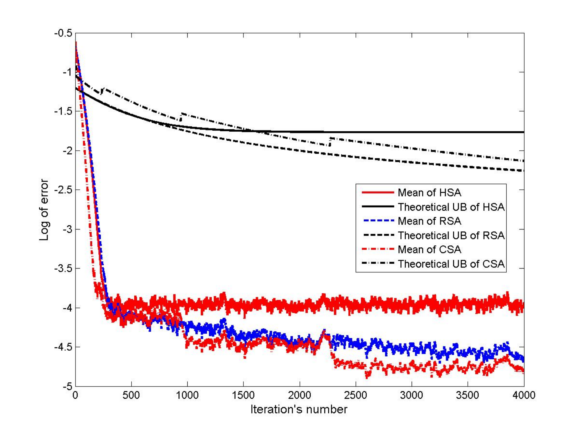
In this section, we interpret the numerical results obtained in the previous subsections, focusing on a comparison between the theoretical and empirical results and the sensitivity of the schemes to the algorithm parameters.

VI-B1 Theoretical and empirical trajectories

In Figures 3a, 3b and 3c, we provide schematics of the trajectories associated with the theoretically obtained upper bounds and the empirical means. Several observations can be immediately made. In the context of the stochastic utility problem and the network utility maximization problem, we observe that the RSA scheme displays uniformly better theoretical bounds, in comparison with CSA. It is also worth emphasizing that the “jumps” seen in the theoretical error bound trajectories of CSA correspond to junctures where the steplengths drop. In fact, the cascading nature is also apparent in the empirical trajectories of the network utility maximization game in Fig 3c, albeit in a less obvious fashion. We observe that the overall empirical behavior of both schemes is similar in terms of the final errors for the utility and network utility maximization problems while in the context of the bimatrix game, the CSA scheme performs significantly better for a subset of problems.

VI-B2 Sensitivity to algorithm parameters

Finally, in this section, we discuss the sensitivity of each scheme to algorithm parameters and provide a comparison with a standard stochastic approximation scheme where we assume that the stepsize is $\gamma_{k}=\frac{\alpha}{k}$ for $k\geq 1$ and $\alpha>0$ . In HSA, we intend to examine the effect of choosing different values of $\alpha$ on the performance of the SA algorithm. In the RSA scheme, we have a choice of the first stepsize $\gamma_{0}^{RSA}$ and also parameter $c$ in the inequality of Proposition 3. We set $c=0.5$ and examine the impact of changing $\gamma_{0}^{RSA}$ . Finally, the CSA scheme performs differently with different choices of the cascading parameter $0<\theta<1$ . We consider three different values for each of $\alpha$ , $\gamma_{0}^{RSA}$ , and $\theta$ and present simulations for HSA, RSA and CSA in the case of the stochastic utility problem. The reference setting is specified by $n=20$ , $N=4000$ , $\epsilon=0.5$ , and $\eta=0.5$ . Now suppose $\alpha$ , $\gamma_{0}^{RSA}$ , and $\theta$ are set as follows:

\alpha=1,0.5,\hbox{ and }0.25;\quad\gamma_{0}^{RSA}=1,0.5,\hbox{ and }0.25;\quad\theta=0.75,0.5,\hbox{ and }0.25.

Figure 4 shows the simulations for the specified parameters. Note that “Th. UB” shows the corresponding theoretical upper bound of each scheme and ”Mean” shows the mean of error $\|z_{k}-z_{\epsilon,\eta}^{*}\|^{2}$ where $z=(x,y)$ .

Figure 4a shows the harmonic scheme with $\alpha=$ 1, 0.5, and 0.25 corresponding to labels 1, 2, and 3 in the legend. This shows that the performance of HSA is extremely sensitive to the choice of $\alpha$ and HSA implementations with a larger $\alpha$ performed better for the stochastic utility problem. Furthermore, the error on termination of HSA schemes can vary by nearly a factor of 10 for the problems that we tested. The update rules in the RSA schemes rely on $\eta$ and $L$ with $\gamma_{0}^{RSA}$ being the sole user input. Yet, when examining the sensitivity of the RSA scheme to the choice of $\gamma_{0}^{RSA}$ (see Figure 4b with $\gamma_{0}^{RSA}=$ 1, 0.5, and 0.25 corresponding to labels 1, 2, and 3), we observe that the performance is relatively insensitive to the choice of initial stepsize. In effect, the modeler can be relatively less concerned about such parameters when attempting to solve this class of problems. Importantly, both theoretical and numerical aspect of RSA have almost the same performance for three values of $\gamma_{0}^{RSA}$ . Finally, a concern in the implementation of CSA schemes is the choice of $\theta$ , the cascading parameter where $\theta\in(0,1)$ . Figure 4c shows the simulation of the cascading scheme with $\theta=$ 0.75, 0.50, and 0.25 corresponding to labels 1, 2, and 3. Theoretically, we observe that smaller values of $\theta$ (more aggressive reductions in stepsize) lead to slightly superior theoretical bounds but not significantly so. However, the results are far more muted when conducting an empirical examination. In particular, we observe that the CSA scheme appears to be relatively insensitive to diversity in the choice of $\theta.$ The relative robustness of the RSA and CSA schemes to the choice of parameters is seen as a crucial advantage of such schemes.

VII Concluding remarks

This paper is motivated by two shortcomings associated with standard stochastic approximation procedures for stochastic convex programs. First, standard implementations of such schemes provide little guidance in specifying parameters that may prove crucial in practical performance. Furthermore, direct extensions to nonsmooth regimes of such schemes is not immediate. Accordingly, this paper makes two sets of contributions. First, we develop two sets of adaptive steplength schemes and provide the associated global convergence theory. Of these, the former, a recursive steplength scheme (RSA), specifies the steplength at a particular iteration using the previous steplength and certain problem parameters. The second scheme, called a cascading steplength scheme (CSA), differs significantly and is essentially a sequence of constant steplength schemes in which the steplength is reduced at specific points in time. The second set of contributions extends these techniques to settings where the objective is not necessarily differentiable. Through the use of a local smoothing method that perturbs the problem through a uniformly distributed random variable, we propose a stochastic gradient scheme. Notably, Lipschitz bounds are obtained for the gradients and their growth with problem size is found to be modest. Locally smoothed variants of the RSA and CSA scheme were seen to perform well on two classes of nonsmooth stochastic optimization problems and implementations were seen to be relatively insensitive to problem parameters.

References

[1] H. Robbins and S. Monro, “A stochastic approximation method,” Ann. Math. Statistics, vol. 22, pp. 400–407, 1951.
[2] Y. M. Ermoliev, “On the stochastic quasi-gradient method and stochastic quasi-feyer sequences,” Kibernetika, Kiev, no. 2, pp. 73–83, 1969.
[3] ——, Stochastic Programming Methods. Moscow: Nauka, 1976.
[4] ——, “Stochastic quasigradient methods and their application to system optimization,” Stochastic, vol. 9, pp. 1–36, 1983.
[5] ——, “Stochastic quasigradient methods,” in Numerical Techniques for Stochastic Optimization. Sringer-Verlag, 1983, pp. 141–185.
[6] J. R. Birge and F. Louveaux, Introduction to Stochastic Programming: Springer Series in Operations Research. Springer, 1997.
[7] A. Ruszczyński and W. Syski, “Stochastic approximation method with gradient averaging for unconstrained problems,” IEEE Trans. Automat. Control, vol. 28, no. 12, pp. 1097–1105, 1983.
[8] B. Polyak and A. Juditsky, “Acceleration of stochastic approximation by averaging,” SIAM J. Control Optim., vol. 30, no. 4, pp. 838–855, 1992.
[9] B. Polyak, “Random algorithms for solving convex inequalities,” in Inherently Parallel Algorithms in Feasibility and Optimization and their Applications, D. Butnariu, Y. Censor, and S. Reich, Eds. Amsterdam, Netherlands: Elsevier, 2001, pp. 409–422.
[10] A. Nemirovski, A. Juditsky, G. Lan, and A. Shapiro, “Robust stochastic approximation approach to stochastic programming,” SIAM Journal on Optimization, vol. 19, no. 4, pp. 1574–1609, 2009.
[11] J. Kiefer and J. Wolfowitz, “Stochastic estimation of the maximum of a regression function,” Annals of Mathematical Statistics, vol. 23, no. 3, pp. 462–466, 1952.
[12] J. C. Spall, “Multivariate stochastic approximation using a simultaneous perturbation gradient approximation,” IEEE Transactions on Automatic Control, vol. 37, no. 3, pp. 332–341, 1992.
[13] S. Bhatnagar, M. C. Fu, and S. I. Marcus, “Convergence of simultaneous perturbation stochastic approximation for nondifferentiable optimization,” IEEE Transactions on Automatic Control, no. 48, pp. 1459–1463, 2003.
[14] V. S. Borkar and S. P. Meyn, “The O.D.E. method for convergence of stochastic approximation and reinforcement learning,” SIAM J. Control Optim., vol. 38, no. 2, pp. 447–469 (electronic), 2000.
[15] V. S. Borkar, Stochastic Approximation: A Dynamical Systems Viewpoint. Cambridge University Press, 2008.
[16] B. Polyak, Introduction to optimization. New York: Optimization Software, Inc., 1987.
[17] H. J. Kushner and G. G. Yin, Stochastic Approximation and Recursive Algorithms and Applications. Springer New York, 2003.
[18] A. Shapiro, “Monte Carlo sampling methods,” in Handbook in Operations Research and Management Science. Amsterdam: Elsevier Science, 2003, vol. 10, pp. 353–426.
[19] J. Linderoth, A. Shapiro, and S. Wright, “The empirical behavior of sampling methods for stochastic programming,” Ann. Oper. Res., vol. 142, pp. 215–241, 2006.
[20] A. S. Nemirovskiĭ and D. B. Judin, “Cesàro convergence of the gradient method for the approximation of saddle points of convex-concave functions,” Dokl. Akad. Nauk SSSR, vol. 239, no. 5, pp. 1056–1059, 1978.
[21] W. Powell, A. A. Ruszczynski, and H. Topaloglu, “Validation analysis of robust stochastic approximation method,” Mathematical Programming (under revision), 2009.
[22] T. Alamo, R. Tempo, and E. Camacho, “Randomized strategies for probabilistic solutions of uncertain feasibility and optimization problems,” IEEE Transactions on Automatic Control, vol. 54, no. 11, pp. 2545–2559, 2009.
[23] A. Nedić, “Random projection algorithms for convex set intersection problems,” 2010, accepted at the 49th IEEE Conference on Decision and Control.
[24] G. Calafiore, F. Dabbene, and R. Tempo, “Randomized algorithms for probabilistic robustness with real and complex structured uncertainty,” IEEE Transactions on Automatic Control, vol. 45, pp. 2218–2235, 2000.
[25] B. T. Polyak and R. Tempo, “Probabilistic robust design with linear quadratic regulators,” Systems and Control Letters, vol. 43, pp. 343–353, 2001.
[26] A. Nedić, “Subgradient methods for convex minimization,” Ph.D. dissertation, Massachussetts Institute of Technology, 2001.
[27] A. Nedić, D. P. Bertsekas, and V. Borkar, “Distributed asynchronous incremental subgradient methods,” in Proceedings of the March 2000 Haifa Workshop on ”Inherently Parallel Algorithms in Feasibility and Optimization and Their Applications”, D. Butnariu, Y. Censor, and S. Reich, Eds., Elsevier, Amsterdam, 2001.
[28] A. Nedić and D. P. Bertsekas, “Convergence rate of incremental algorithms,” Stochastic Optimization: Algorithms and Applications, pp. 223–264, 2001.
[29] S. S. Ram, A. Nedić, and V. V. Veeravalli, “Incremental stochastic subgradient algorithms for convex optimization,” SIAM Journal on Optimization, vol. 20, no. 2, pp. 691–717, 2009.
[30] ——, “Distributed stochastic subgradient projection algorithms for convex optimization,” Journal of Optimization Theory and Applications, vol. 147, no. 3, pp. 516–545, 2010.
[31] ——, “Asynchronous gossip algorithms for stochastic optimization,” 2009, proceedings of the 48th IEEE Conference on Decision and Control, Shanghai, China.
[32] F. Facchinei and J.-S. Pang, Finite-dimensional variational inequalities and complementarity problems. Vols. I,II, ser. Springer Series in Operations Research. New York: Springer-Verlag, 2003.
[33] H. Jiang and H. Xu, “Stochastic approximation approaches to the stochastic variational inequality problem,” IEEE Transactions Automatic Control, vol. 53, no. 6, pp. 1462–1475, 2008.
[34] J. Koshal, A. Nedić, and U. V. Shanbhag, “Single timescale regularized stochastic approximation schemes for monotone nash games under uncertainty,” Proceedings of the IEEE Conference on Decision and Control (CDC), 2010.
[35] A. Juditsky, A. Nemirovski, and C. Tauvel, “Solving variational inequalities with stochastic mirror-prox algorithm,” 2008, http://arxiv.org/abs/0809.0815.
[36] R. M. Van Slyke and R. Wets, “L-shaped linear programs with applications to optimal control and stochastic programming,” SIAM J. Appl. Math., vol. 17, pp. 638–663, 1969.
[37] A. Ruszczynski, “Decomposition methods,” in Handbook in Operations Research and Management Science. Amsterdam: Elsevier Science, 2003, vol. 10, pp. 141–212.
[38] A. Kulkarni and U. Shanbhag, “Recourse-based stochastic nonlinear programming: Properties and Benders-SQP algorithms,” To appear in Computational Optimization and Applications, 2010.
[39] U. V. Shanbhag, G. Infanger, and P. W. Glynn, “A complementarity framework for forward contracting under uncertainty,” to appear in Operations Research.
[40] D. P. Bertsekas and J. N. Tsitsiklis, “Gradient convergence in gradient methods,” SIAM Journal on Optimization, vol. 10, no. 3, pp. 627–642, 2000.
[41] H. Jiang and D. Ralph, “Smooth SQP methods for mathematical programs with nonlinear complementarity constraints,” SIAM Journal on Optimization, vol. 10, no. 3, pp. 779–808, 2000.
[42] F. Facchinei, H. Jiang, and L. Qi, “A smoothing method for mathematical programs with equilibrium constraints,” Math. Program., Ser. A, vol. 85, no. 1, pp. 107–134, 1999.
[43] A. M. Gupal, Stochastic methods for solving nonsmooth extremal problems (Russian). Naukova Dumka, 1979.
[44] H. Lakshmanan and D. Farias, “Decentralized resource allocation in dynamic networks of agents,” SIAM Journal on Optimization, vol. 19, no. 2, pp. 911–940, 2008.
[45] W. Powell, A. A. Ruszczynski, and H. Topaloglu, “Learning algorithms for separable approximations of discrete stochastic optimization problems,” Mathematics of Operations Research, vol. 29, no. 1, pp. 814–836, 2004.
[46] D. P. Bertsekas, “Stochastic optimization problems with nondifferentiable functionals with an application in stochastic programming,” in Proceedings of 1972 IEEE Conference on Decesion and Control, 1972, pp. 555–559.
[47] ——, “Stochastic optimization problems with nondifferentiable cost functionals,” Journal of Optimization Theory and Applications, vol. 12, no. 2, pp. 218–231, 1973.
[48] K. L. Chung, “On a stochastic approximation method,” Ann. Math. Statistics, vol. 25, pp. 463–483, 1954.
[49] J. Sacks, “Asymptotic distribution of stochastic approximation procedures,” Ann. Math. Statist., vol. 29, pp. 373–405, 1958.
[50] H. Kesten, “Accelerated stochastic approximation,” Ann. Math. Statist, vol. 29, pp. 41–59, 1958.
[51] H. J. Kushner and T. Gavin, “Extensions of Kesten’s adaptive stochastic approximation method,” Ann. Statist., vol. 1, pp. 851–861, 1973.
[52] B. Delyon and A. Juditsky, “Accelerated stochastic approximation,” SIAM J. Optim., vol. 3, no. 4, pp. 868–881, 1993.
[53] J. H. Venter, “An extension of the Robbins-Monro procedure,” Ann. Math. Statist., vol. 38, pp. 181–190, 1967.
[54] T. L. Lai and H. Robbins, “Adaptive design and stochastic approximation,” Ann. Statist., vol. 7, no. 6, pp. 1196–1221, 1979.
[55] C. Z. Wei, “Multivariate adaptive stochastic approximation,” Ann. Statist., vol. 15, no. 3, pp. 1115–1130, 1987.
[56] J. C. Spall, “Adaptive stochastic approximation by the simultaneous perturbation method,” IEEE Trans. Automat. Control, vol. 45, no. 10, pp. 1839–1853, 2000.
[57] ——, “Feedback and weighting mechanisms for improving Jacobian estimates in the adaptive simultaneous perturbation algorithm,” IEEE Trans. Automat. Control, vol. 54, no. 6, pp. 1216–1229, 2009.
[58] S. Bhatnagar, “Adaptive multivariate three-timescale stochastic approximation algorithms for simulation based optimization,” ACM Transactions on Modeling and Computer Simulation, pp. 74–107, 2005.
[59] ——, “Adaptive newton-based multivariate smoothed functional algorithms for simulation optimization,” ACM Transactions on Modeling and Computer Simulation, Accepted for Publication, 2007.
[60] D. P. Bertsekas and S. K. Mitter, “A descent numerical method for optimization problems with nondifferentiable cost functionals,” SIAM J. Control, vol. 11, pp. 637–652, 1973.
[61] K. C. Kiwiel, Methods of descent for nondifferentiable optimization, ser. Lecture Notes in Mathematics. Berlin: Springer-Verlag, 1985, vol. 1133.
[62] Z.-Q. Luo, J.-S. Pang, and D. Ralph, Mathematical programs with equilibrium constraints. Cambridge: Cambridge University Press, 1996.
[63] V. A. Steklov, “Sur les expressions asymptotiques decertaines fonctions définies par les équations différentielles du second ordre et leers applications au problème du dévelopement d’une fonction arbitraire en séries procédant suivant les diverses fonctions,” Comm. Charkov Math. Soc., vol. 2, no. 10, pp. 97–199, 1907.
[64] ——, Main Problems of Mathematical Physics. Nauka, Moscow, 1983.
[65] V. I. Norkin, “The analysis and optimization of probability functions,” International Institute for Applied Systems Analysis technical report, Tech. Rep., 1993, wP-93-6.
[66] R. T. Rockafellar and R. J.-B. Wets, Variational analysis, ser. Grundlehren der Mathematischen Wissenschaften [Fundamental Principles of Mathematical Sciences]. Berlin: Springer-Verlag, 1998, vol. 317.
[67] Y. Ermoliev and E. A. Nurminski, “Limit extrernal problems,” Kibernetika, vol. 4, pp. 130–132, 1973.
[68] A. Gaivoronski, “On nonstationary stochastic optimization problems,” Kibernetika, pp. 89–92, 1978.
[69] A. M. Gupal and V. I. Norkin, “An algorithm for the minimization of discontinuous functions,” Kibernetika, pp. 73–75, 1977.
[70] U. Ravat and U. V. Shanbhag, “On the characterization of solution sets of smooth and nonsmooth stochastic nash games,” in Proceedings of the American Control Conference (ACC), Baltimore, 2010.
[71] R. T. Rockafellar, Convex Analysis. Princeton, New Jersey: Princeton University Press, 1970.
[72] A. Nedić and A. Ozdaglar, “Subgradient methods for saddle-point problems,” Journal of Optimization Theory and Applications, vol. 142, no. 1, pp. 205–228, 2009.
[73] F. Kelly, A. Maulloo, and D. Tan, “Rate control for communication networks: shadow prices, proportional fairness, and stability,” Journal of the Operational Research Society, vol. 49, pp. 237–252, 1998.
[74] R. Srikant, Mathematics of Internet Congestion Control. Birkhauser, 2004.

On Stochastic Gradient and Subgradient Methods with Adaptive Steplength Sequences

Abstract

I Introduction

II Problem Formulation and Background

II-A Problem Formulation

Assumption 1

Assumption 2

Lemma 1

Lemma 2

II-B Adaptive Stochastic Approximation Schemes

II-C Smoothing Techniques

Definition 1

III A recursive steplength stochastic approximation scheme

III-A Preliminaries

Proposition 1 (Almost-sure convergence)

Proof:

Lemma 3

Proof:

Assumption 3

Lemma 4 (Strongly convex function with Lipschitz gradients)

Proof:

III-B A recursive steplength scheme

Proposition 2

Proof:

III-C Convergence theory

Proposition 3 (Global convergence of RSA scheme)

Proof:

Corollary 1 (Convergence of RSA scheme)

Proof:

Proposition 4 (Convergence of RSA with a nonsmooth objective)

Proof:

IV A cascading steplength stochastic approximation scheme

IV-A A cascading steplength scheme

Proposition 5

Proof:

Lemma 5

Proof:

Proposition 6

Proof:

IV-B Global convergence theory

Lemma 6

Proof:

Proposition 7 (Cascading steplength stochastic approximation (CSA) scheme)

Proof:

V Addressing nondifferentiability through Local Randomized Smoothing

V-A Differentiable Approximation

Assumption 4

Lemma 7

Proof:

V-B Smoothing via random variables with uniform distributions

Lemma 8

Proof:

V-C Convergence analysis of the algorithm with local smoothing

V-C1 Deterministic nondifferentiable optimization

Proposition 8

Proof:

V-C2 Stochastic nondifferentiable optimization

Lemma 9

Proof:

Proposition 9

Proof:

VI Numerical results

VI-A Examples

VI-A1 A stochastic utility problem

VI-A2 A bilinear matrix game problem

VI-A3 A stochastic network utility problem

VI-B Interpretation of numerical results

VI-B1 Theoretical and empirical trajectories

VI-B2 Sensitivity to algorithm parameters

VII Concluding remarks

References

On Stochastic Gradient and Subgradient Methods
with Adaptive Steplength Sequences