Behavior of Graph Laplacians on Manifolds with Boundary
Abstract
In manifold learning, algorithms based on graph Laplacians constructed from data have received considerable attention both in practical applications and theoretical analysis. In particular, the convergence of graph Laplacians obtained from sampled data to certain continuous operators has become an active research topic recently. Most of the existing work has been done under the assumption that the data is sampled from a manifold without boundary or that the functions of interests are evaluated at a point away from the boundary. However, the question of boundary behavior is of considerable practical and theoretical interest. In this paper we provide an analysis of the behavior of graph Laplacians at a point near or on the boundary, discuss their convergence rates and their implications and provide some numerical results. It turns out that while points near the boundary occupy only a small part of the total volume of a manifold, the behavior of graph Laplacian there has different scaling properties from its behavior elsewhere on the manifold, with global effects on the whole manifold, an observation with potentially important implications for the general problem of learning on manifolds.
1 Introduction
Graph Laplacian constructed from data points is a key element in many machine learning algorithms including spectral clustering, e.g., [uvon], semi-supervised learning [zhu2006semi, chapelle2006ssl] and dimensionality reduction [BelkinLapMap2003], as well as a number of other applications. A large amount of work in recent years has been centered on analyzing various theoretical aspects of graph Laplacians on manifolds, and, in particular, on their different modes of convergence, when the data goes to infinity and/or the parameters, such as kernel bandwidth, tend to zero [belkinThesis, lafon, hein, CoifmanLafon2006, singer, gine, Hein07graphlaplacians, belkin2008, uvon2008, rosasco2010]. A typical result in that direction shows that the discrete graph Laplacian converges11 1 Different modes of convergence are possible here, such as different types of pointwise or uniform convergence or convergence of eigenvectors. to the Laplacian-Beltrami operator on manifolds when the bandwidth parameter of the kernel is chosen as an appropriate function of the number of data points. These results help to clarify our understanding of the underlying objects, to shed light on properties of the algorithms and to guide the selection of algorithms in practical applications.
For example, an analysis of normalized versus unnormalized Laplacians in [uvon2008]) suggests that normalization may be preferable in practical applications. In another example, the estimators of several graph Laplacian based semi-supervised learning algorithms had recently been shown to converge to constant solutions in the limit of infinite unlabeled points while fixing labeled points [nadler2009], suggesting the use of iterated Laplacians [Zhou2011a], which indeed shows superior performance in practice.
The spectral convergence of a graph Laplacian is another important limit analysis of the graph Laplacian, which links directly to applications. The empirical spectral convergence of spectral clustering when the sample size goes to infinity for a fixed kernel bandwidth was studied by [uvon2008], while the spectral convergence of a graph Laplacian to the Laplace-Beltrami operator when the kernel bandwidth goes to zero as goes to infinity is studied in [belkinCLEM].
However, most previous results on graph Laplacians deal with the setting where the manifold does not have a boundary or when the operator is analyzed at a point away from the boundary. Arguably, it is a significant short-coming of these analyses, since manifolds or domains with boundary are present explicitly or implicitly in many problems of significant interest in data analysis. Perhaps the simplest example is the fact that the pixel intensity of a gray-scale image cannot be smaller than zero, providing a natural boundary condition for any image manifolds. A more interesting example is in motion analysis, where the manifold of configurations of a human or robot body (perhaps embedded using video images or data from sensors attached to limbs) has boundaries corresponding to the limits for the range of motions of each individual joint. More generally, it is natural to think that boundaries in data are present whenever the generating process itself is in some way constrained. It is clear that if such manifolds are to be learned from data, the boundary behavior cannot be disregarded.
In the current paper we discuss the boundary behavior of graph Laplacians by analyzing the graph Laplacian convergence at the boundary. We show that the graph Laplacian at the boundary converges to a gradient operator in the direction normal to the boundary, when the bandwidth parameter is chosen adaptively as a function of the number of data points. We provide explicit bounds for the convergence. One of the key results of our analysis is that both the behavior and the scaling of the graph Laplacian near the boundary is quite different from that in the interior of the manifold. Specifically, for a fixed function and a small bandwidth parameter the (appropriately scaled) graph Laplacian will be close to the Laplace-Beltrami operator on interior point , while at the boundary the same object will be close to the normal derivative . We see that the large values of the graph Laplacian applied to a fixed function are likely to correspond to the boundary points. Moreover, the analysis shows that while there are few points near the boundary of a manifold, their influence on the graph Laplacian is disproportionately large and cannot be ignored. This suggests that the boundary has a global effect on the graph Laplacian, a finding that is confirmed by our numerical experiments provided in the paper. Viewed in a different way it suggests that for algorithms when a graph Laplacian is used as a regularizer, as is the case in many applications, bounding the norm would lead to the suppression of the large values near the boundary. Thus the minimizer of the regularization problem (or similarly, the eigenvectors) should satisfy the Neumann boundary conditions, i.e., be nearly constant in the direction orthogonal to the boundary, which is confirmed by our numerical experiments.
In a related line of investigation we find that the symmetric normalized graph Laplacian has a different boundary behavior from the random walk (asymmetric normalized) and unnormalized graph Laplacians. Unlike those two, for a fixed function , converges to for a boundary point , where is the probability density function. This does not lead to the Neumann boundary condition, and seems strange from a practical point of view.
As a further illustration of the importance of boundary conditions in learning theory, we explore the boundary effects for a reproducing kernel in a simple 1-dimensional example. We also discuss the limit of the graph Laplacian regularizer on manifolds with boundary, which cannot be taken for granted to be the same as the limit on or manifolds without boundary because of the boundary behavior of graph Laplacians.
Finally we briefly compare the graph Laplacian built from random samples to the Laplacian on regular grids in numerical PDE’s.
1.1 Problem Setting
We now proceed with a more technical setting of the problem. Let be a compact Riemannian submanifold of intrinsic dimension embedded in , the interior of , and the boundary of , which we will assume to satisfy the necessary smoothness conditions22 2 Instead of spending several pages to describe these smoothness conditions in this paper, we refer readers to [belkinThesis, lafon, hein] for more details.. Given random samples drawn i.i.d. from a distribution with a smooth density function on such that , we can build a weighted graph by mapping each sample point to vertex and assigning a weight to edge . One typical weight function is the Gaussian defined as , which is used in this paper. Let the matrix be the edge weight matrix of graph with , and be a diagonal matrix such that , then the unnormalized graph Laplacian is defined as matrix
| (1) |
There are several ways of normalizing . For instance, the most commonly used two are the asymmetric random walk normalized version and the symmetric normalized version .
Another useful way of building a graph Laplacian is governed by a parameter such that we first normalize as , then define the unnormalized, random walk and symmetric normalized graph Laplacians as
| (2) |
where is the corresponding diagonal degree matrix for . It is easy to see when , these graph Laplacians become the commonly used ones without the first step normalization. Therefore, for each value of , there are three closely connected empirical graph Laplacians.
The limit study of graph Laplacians primarily involves the limits of two parameters, sample size and weight function bandwidth . As increases, one typically decreases to let the graph Laplacian capture progressively a finer local structure.
With a proper rate as a function of and , the limit of for a given smooth function and fixed can be shown to be when is a compact submanifold of without boundary and is a uniform density. This builds a connection between the discrete graph Laplacian and the continuous Laplace-Beltrami operator on manifolds, which in can be written as
| (3) |
This connection is an important step in providing a theoretical foundation for many graph Laplacian based machine learning algorithms. For instance, harmonic functions used in [zhu2003] for semi-supervised learning is in fact a solution of a Laplace equation, with a “point boundary condition” at labeled points.
The limit of and its various aspects, including the finite sample analysis, are studied in [belkinThesis, lafon, hein, singer, gine, Hein07graphlaplacians, belkin2008, belkinCLEM]. The basic result is that the limit of for is (up to a constant )
| (4) |
where is the weighted Laplacian and . These papers deal with the analysis of graph Laplacians at an interior point of the manifold and do not deal with boundary behavior. The exception to that is the analysis in [CoifmanLafon2006], which includes manifolds with boundary, assuming the Neumann boundary conditions on the space of functions. Specifically, the Taylor series for the Gaussian convolution in [CoifmanLafon2006, Lemma 9] involves a term containing the normal gradient at the boundary, which can be reformulated to obtain the limit for the graph Laplacian on the manifold boundary. However, there is no explicit discussion of the boundary behavior as well as its implication for learning in [CoifmanLafon2006]. Discrete graph Laplacian is not considered in that work. We believe that given the popularity of graph Laplacians in machine learning, the boundary behavior of graph Laplacians deserves a more detailed study.
In Section 2, we state some existing results on the limit analysis of the graph Laplacian as well as some necessary preparatory results, which will be useful for our analysis. Section 3 contains our main Theorem 2, which states that near the boundary, the graph Laplacian converge to the normal gradient and shows the scaling behavior and explicit rates of convergence. We also show how the scaling changes between the boundary and the interior points of the manifold. Numerical examples to support our analyses are provided in Section 4. Several important implications of the boundary behavior of the graph Laplacian are discussed in Section 5.
2 Technical Preliminaries
In this section, we review the existing limit analysis of graph Laplacians , and on points away from the boundary of a compact submanifold. We also provide some technical results useful for our analysis in Section 3.
Given an undirected graph representation of the random sample set of size , the weight function with parameter is defined as
| (5) |
Notice that in this Gaussian weight function, the Euclidean distance should be used, instead of other distance, e.g., the geodesic on manifolds. It is this critical feature that on one hand makes the graph Laplacians computationally attractive, on the other hand has important implications, which will be discussed in the rest this paper.
Define the corresponding discrete degree function as
| (6) |
Then we first normalize the weight function to obtain
| (7) |
Note that this weight function also depends on the locations of and other than the Euclidean distance . We use the three subscripts to emphasize the related parameters. The corresponding discrete degree function is
| (8) |
If the weight matrix for is and the corresponding degree matrix is , then the normalized weight matrix is
| (9) |
By finding the corresponding degree matrix , the unnormalized graph Laplacian is
| (10) |
and the other two normalized versions are defined accordingly as and .
For a fixed smooth function , and any (including the samples and unseen points), define as the following,
| (11) |
and similarly for the random walk normalized graph Laplacian
| (12) |
For , it can be shown that where . Similar notions also apply to the degree functions. The intuition is that we treat vector as a sampled continuous function on . As , the vector becomes “closer and closer” to .
Three useful convergence results for the interior points will be needed in our analysis [Hein07graphlaplacians]:
| (13) |
where , and
| (14) |
The following limit shows that the graph Laplacian on points that are away from the boundary converge to the density weighted Laplace-Beltrami operator with a proper rate of and .
| (15) |
where . The limits of and can be found in [Hein07graphlaplacians]
On a -dimensional smooth manifold , for an interior point , the small neighborhood around is locally equivalent to whole space , while for a point on the boundary of , i.e. , the small neighborhood around is locally mapped into a half space defined as . This is a key fact that will be used in this paper.
Next we will need a concentration inequality for the finite sample analysis of the graph Laplacian.
Lemma 1
(McDiarmid’s inequality) Let , be i.i.d. random variables of from density , , and satisfies
| (16) |
then
| (17) |
3 Analysis of Graph Laplacian Near Manifold Boundary
In this section, we analyze the limits of the Laplacians , and when is on or near the boundary of manifold . The argument roughly follows the lines of the convergence arguments in [belkinThesis, hein, CoifmanLafon2006].
To fix the notation, in the rest of this paper, we use expressions without subscript to indicate the corresponding limit as , and expressions without subscript to for the limits as .
| (18) |
For smooth and ,
| (19) |
and
| (20) |
Similarly, can be rewritten as with .
Next we show the limits of the graph Laplacians on boundary point as and at a proper rate, when has a smooth boundary.
Theorem 2
Let , , , , be a smooth boundary of , , and be sufficiently small, then for the unnormalized graph Laplacian
| (21) |
for the random walk normalized graph Laplacian
| (22) |
and for the symmetric normalized graph Laplacian
| (23) |
where , n is inward normal direction, only depends on and , , and .
Proof: We first show the limit of the expectation of as in step 1 to 3. Then the limit of and can easily be found with the help of the limit of discrete degree function . At last, we obtain the finite sample results by applying Lemma (1).
For a sufficiently small , let be the set of points that are within distance from the boundary (a thin layer of “shell”), and . We first show that for a small , is approximated by two different terms on and , and more importantly these two terms have different orders of . Then together with the limit of , we can find the limit of and .
Step 1: The key step for the limit analysis of graph Laplacians is the approximation on the manifold. Consider
| (24) |
This integral is on the manifold . In order to study the the limit of this integral when , we can approximate the integral on an unknown smooth manifold by an integral on its tangent space at each point when is small such that the approximation errors of each step are comparable. For , the tangent space is the whole space , while for , the tangent space is the half space ().
When is within an Euclidean ball of radius centered at , in the local coordinate around a fixed , the origin is point , and let be the local geodesic coordinate of , be the projection of on the tangent space at . Then we have the following important approximation (see [belkinThesis, Chapter 4.2] and [CoifmanLafon2006, Appendix B]).
| (25) |
Step 2: Now we are ready to approximate each of the five terms in integral (24) when the integral is taken inside a ball centered at having radius in norm. Notice that .
| (26) |
where is the Hessian of at point . Notice that, the order inside of the big oh is determined by the larger one between the approximation error of to which is , and the Taylor expansion error on manifold as a function of . The other observation is that, the order of the product of these terms is determined by the third term (), the highest order of which is , with the next ones as and . This means it is enough to keep the approximation terms up to order .
Combing all the approximation together in a ball of radius around , with a change of variable , we can obtain
| (27) |
where is a ball of radius in norm centered at , while is a ball of radius in norm, and is the tangent space at point . For a sufficiently small , the first step replaces the integral over the whole with ball , generating an error [CoifmanLafon2006, Appendix B]. Then this integral is the same as the integral over a ball on the manifold . Finally, for an interior point , , which means function is a even function of . When taking the integral, the first term which has order is odd and therefore vanishes. Then the three left terms that are of order inside the integral are exactly the weighted Laplacian at , which is of order . For a boundary point , . Next we study the interior points.

Step 3: In Figure. 1, (the “shell”) is a point near the boundary, n is the inward normal direction, and is the nearest boundary point to along n. In the local coordinate system, is the origin, and along the normal direction the Gaussian convolution is from to , which is not symmetric. Therefore, is not an even function in the normal direction, so the highest order term is the order term.
In this case, all the odd terms of still will vanish in all directions except the normal direction n, and the most important point is that the leading term along the normal direction is of order , while for interior points it is . Next we assume is the normal direction.
| (28) |
where is the distance to the nearest point of on the boundary along the normal direction () as shown in Figure 1. When , in the local coordinate system
| (29) |
where , . This result also needs the following limits, which generalize [hein, Proposition 2.33] to points on the boundary.
| (30) |
Step 4: The normalized graph Laplacians can be obtained by normalization through . Then the limit of the random walk normalized graph Laplacian is (we include the limit for interior point for comparison)
| (31) |
As for the limit of , it can be shown that where . Then the limit analysis follows easily.
Step 5: Consider
| (32) |
Notice that in the sum, different terms are not independent, since the degree and includes sums of all the random variables. Therefore, we need to use the McDiarmid’s inequality in this step. The maximum change if we change a random variable is bounded by
| (33) |
The maximum change happens when we move a point from a high density region with a minimum function value to a point in a low density region with a maximum function value. Similar analyses apply to normalized graph Laplacians. Then We conclude the proof by applying the McDiarmid’s inequality.
Notice that the error rate essentially comes from the McDiarmid’s inequality. When , all terms in equation (32) are i.i.d., then we can use the Bernstein’s inequality to obtain a better rate for . For , an even better rate can be obtained as shown by [singer]. When , although strictly speaking the terms in equation (32) are not i.i.d., since is really an average of all the samples, it is almost a function of alone, and a function of alone. Then in this case, we believe it is possible to obtain a better error rate.
Together with the existing analysis for interior points, we have the following implication of Theorem (2)
| (34) |
Therefore, the graph Laplacian converges to a different limit on from that on . More importantly, these two limits are of different orders, one is while the other is . However, in practice, when we apply the normalization step, we do not know where the boundary is, and always apply a global normalization for all in order to obtain the weighted Laplacian in the limit. For a small
| (35) |
Notice that the error only happens on a “shell” having volume . For such that on the boundary point with enough data points, we have that for small values of
| (36) |
4 Numerical Examples
In this section, we explore the boundary behavior of the graph Laplacian by studying numerical examples.


4.1 Graph Laplacian on the Boundary
Example 1. We take , and . The values of with for points sampled from a uniform distribution (equal-spaced points) and are shown in Panel (a) in Figure (2). As expected, we see that the values at the boundary are much larger than those inside the domain and are consistent with (the value at is roughly -times of the value at ) up to a scaling factor33 3 The positive value at is the result of the normal direction pointing inward (left)..
In Panel (b) we show the interior of the interval where the function is indeed the Laplacian up to a scaling factor. In Panel (c) we analyze the scaling of the graph Laplacian on the boundary as a function of in the log-log coordinates. We see that is close to a linear function of with slope approximately as you would expect from the scaling factor .
Example 2. Next we analyze the boundary behavior for a simple low dimensional manifold. Let be half a unit sphere (), which is a -dimensional submanifold in . The boundary is a unit circle . We take , then the negative inward normal gradient on the boundary is
| (37) |
where is the gradient of , and is the inward normal direction. This means the negative normal gradient of along the inward normal direction on the boundary of a half sphere is a linear function in with a negative slope.
We generate a uniform sample set of points on a half sphere and compute a vector with , . We pick the set to be points near the boundary. The dependence between and for data points sampled from the uniform distribution on the half sphere is plotted in Figure (3) and is consistent with our expectation.

To provide a more rigorous error analysis we compute the mean square errors for several values of and sample size . The results are shown in Table (1). We see that the errors are relatively small compared to the values of the gradient and generally decrease with more data.
| 64/64 | 32/64 | 16/64 | 8/64 | 4/64 | 2/64 | 1/64 | |
|---|---|---|---|---|---|---|---|
| 500 | 0.0090 | 0.0059 | 0.0071 | 0.0136 | 0.0287 | 0.0500 | 0.0725 |
| 1000 | 0.0089 | 0.0048 | 0.0033 | 0.0061 | 0.0121 | 0.0294 | 0.0627 |
| 2000 | 0.0113 | 0.0076 | 0.0073 | 0.0068 | 0.0159 | 0.0356 | 0.0585 |
| 4000 | 0.0083 | 0.0044 | 0.0036 | 0.0044 | 0.0072 | 0.0189 | 0.0516 |
4.2 Comparison to Numerical PDE’s
From previous analysis we can see that, for graph Laplacians, the “missing” edges going out of the manifold boundary on one hand can be seen as being reflected back into , which is particularly intuitive in symmetric NN graphs, see e.g., [maier2009], on the other hand, it can be seen that function values on edges going out of are constant along the normal direction. The latter view is commonly used in schemes of numerical PDE’s in finite difference methods for the Neumann boundary condition, see e.g., [allaire].

We use an example in to show how the Neumann boundary condition for a Laplace operator on a regular grid is implemented in finite difference method, which we hope can shed light on the graph Laplacian on random points. The Laplace operator in is , and the regular grid near the boundary is shown in Figure (4). Since we can separate the Laplacian into partial derivatives of different dimensions, the discrete Laplace matrix on the regular grid with the Neumann boundary condition near along direction can be shown to be
where we only connects points that are next to each other. Along direction the Laplace matrix elements near are . Let the distance between data points be . Consider point on the boundary, along direction, we have a 3-point stencil along axis, , which is enough to define .
This is also true for points that are in the interior , e.g. , , etc. However, for on the boundary along direction (normal direction at ) we only have two points
This shows that “converge” to for on the boundary while to for inside of the domain, with a different scaling behavior. This is almost the same as what happens to the graph Laplacian on random samples. Notice in numerical PDE’s we also have that if , as , . In fact, if we construct the graph Laplacian matrix by setting if two points are next to each other and otherwise, on two dimensional grid as shown in Figure (4), the graph Laplacian matrix is the same as the Laplace matrix with the Neumann boundary condition in numerical PDE’s.
In order to let converges to for all on domain with a single normalization term, we can add a ‘fictitious’ point along the normal direction, and let . Then as we have
Together with direction, we have , . Condition then becomes
which is the Neumann boundary condition. This method is used to implement the Neumann boundary condition in finite difference methods for PDE’s, see e.g., [allaire, Chapter 2].
The graph Laplacian can be seen as an implementation of the Neumann Laplacian on random points, which generalizes regular grids to random graphs based on random samples. This also means by construction, the graph Laplacian is a Neumann Laplacian, which is a built-in feature of the graph Laplacian.
5 Discussions and Implications
5.1 Neumann Boundary Condition
Our analysis of the boundary behavior suggests that the eigenfunctions of both and as well as solutions of certain regularization problems should satisfy the Neumann boundary condition. However, this is not true for the symmetric normalized Laplacian .
Unnormalized and Random Walk Normalized Graph Laplacians: These two versions of graph Laplacians only differ in the density weight outside of the normal gradient, so we only need to find the boundary condition for one of them. Let and be the right eigenfunctions of , then for any positive integer and , the following Neumann boundary condition holds.
| (38) |
This is also true for the eigenfunctions of , the limit of the unnormalized graph Laplacian, which can be seen as follows. All the eigenfunctions should satisfy
On the boundary
Since for all , if does not satisfy the Neumann boundary condition, then on the boundary, therefore such can not be the eigenfunctions of . This implies that all the eigenfunctions of should satisfy the Neumann boundary condition, i.e., for . Similarly, this is true for the unnormalized graph Laplacian with a bounded density.
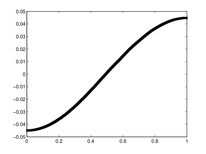


We numerically compute the second and third eigenfunctions of with in Figure (5)44 4 The Neumann boundary condition also holds for other .. The left panel shows the eigenfunctions over interval with a uniform density, while the right panel is for a mixture of two Gaussians. As the numerical results suggest, the second and third eigenfunctions of the graph Laplacian satisfy the Neumann boundary condition, and this is also true for other eigenfunctions. In fact for a uniform over , the Neumann eigenfunctions for the Laplacian are where . The second and third eigenfunctions correspond to and , up to a change of sign, which is consistent with the numerical results in the left panel of Figure (5).
Symmetric Normalized Graph Laplacian: For the symmetric normalized graph Laplacian , the Neumann boundary condition does not hold for its eigenfunctions in the limit. This can be shown by a one to one correspondence between the eigenfunctions of and . Let the eigenvectors for be , and the right eigenvectors for be , then
This is true for any sample size and any parameter . Therefore, in the limit
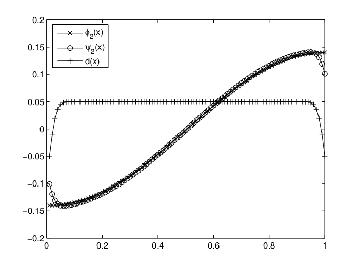
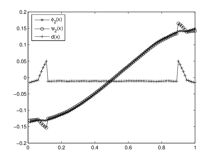
Near the boundary along the normal direction, degree function decreases as a result of the asymmetric interval for , so tends to be “bent” towards zero near the boundary. Since how the graph is constructed will determine what the degree function will be, the boundary behavior also depends on what graph is used. We test two graphs, NN graph and symmetric NN graph, which are studied by [maier2009] for clustering. In the left panel of Figure (6), is scaled and shifted to fit the plot and an NN graph is used. For near the boundary, the degree function decreases as a result of having less points in the fixed radius neighborhood. Therefore, is “bent” towards zero.
Notice that for the symmetric NN graph, in the right panel of Figure (6), the eigenfunctions can have “bumps” near the boundary. This is the result that for symmetric NN graphs, the edges going out of the boundaries are “reflected” back. For example consider in a symmetric NN graph, with the distance between points set as , for point , its nearest neighbors are . However, for point , is not in its nearest neighbors. This means the constructed graph will not be symmetric. If we add for every asymmetric edge , then although the graph is symmetric now, for point will be much larger than other points. As decreases, this “bumps” will shift to the boundary.
5.2 Limit of Graph Laplacian Regularizer
The following graph Laplacian regularizer is a popular penalty term in many semi-supervised learning algorithms when .
| (39) |
This limit is studied in [hein, Chapter 2] without considering the boundary, and is also studied on by [bousquet], which has no boundary and is not a low dimensional manifold either. From Theorem (2), we see that the graph Laplacian has a limit of different scaling behavior on the boundary points compared to the interior points. This leads to the question of the limit of the graph Laplacian regularizer when it is defined on a compact submanifold with a smooth boundary. Based on the quadratic form, we use a similar method as the proof of Theorem (2) to obtain the next theorem.
Theorem 3
For a fixed function , and let , , and the intrinsic dimension of be , then as , and ,
| (40) |
where .
Proof: Following the proof of Theorem (2), let be a thin lay of “shell” of width , and . For a fixed , consider the quadratic form (39), the limit as is
| (41) |
Then by the approximation on manifolds (25) and (26), for a fixed ,
| (42) |
Notice that in this case, the highest order is controlled by , which is of order , and is the tangent space at . Then for any point , the limit is
| (43) |
where
| (44) |
with as the distance between and the nearest boundary point along the normal direction.
On , for a small , we can replace with , then the integral on is
| (45) |
where the coefficient becomes a constant independent of .
On the shell , as , the shell shrinks into a set with measure zero. As long as the function inside the integral is bounded, the integral on will also be zero. For , we have and
| (46) |
For and any , in any direction, . The density is also bounded, therefore, the integral on is zero as . Overall, as , , , and becomes , therefore,
| (47) |
Next consider
| (48) |
Since all the terms in the sum are not i.i.d., we use the McDiarmid’s inequality. The maximum change of replacing one random variable is
| (49) |
therefore,
| (50) |
We conclude the proof by plugging in and .
One important implication of this theorem is that, in order to use a gradient penalty term w.r.t. to different density weights in the form of in the limit, we can use with different values. For instance, to obtain instead of having as the commonly used penalty term , we can set . This penalty then fits the fact that sample are drawn from density .
We tested Theorem (3) numerically on several functions with a uniform density over -dimensional interval . equal-space points are generated, the value of is between and , and we compute the numerical graph Laplacian approximation , and the analytical value of . The ratios of the two are reported in Table (2) and the coefficient plots as a function of are shown in Figure (7).
| \ | |||||||||
|---|---|---|---|---|---|---|---|---|---|
| 0 | 0.4424 | 0.4424 | 0.4424 | 0.4420 | 0.4423 | 0.4424 | 0.4423 | 0.4426 | 0.4431 |
| 1/2 | 0.2497 | 0.2497 | 0.2497 | 0.2497 | 0.2497 | 0.2497 | 0.2497 | 0.2497 | 0.2500 |
| 1 | 0.1411 | 0.1411 | 0.1411 | 0.1412 | 0.1411 | 0.1412 | 0.1410 | 0.1411 | 0.1410 |
| -1 | 1.3845 | 1.3846 | 1.3846 | 1.3819 | 1.3840 | 1.3827 | 1.3865 | 1.3859 | 1.3921 |
In Figure (7), eight different functions from Table (2) are tested for the coefficient using different bandwidth . Each plot corresponds to one fixed value. As suggested by the figure, in Table (2), the maximum values from different are reported. From both the figure and the table we can see that, the numerical results are close to the theoretical coefficient . The figure also suggests a numerically stable patterns as decreases, until it is too small and loses numerical precision.


Notice that on finite samples, it is also possible to treat as an inner product as . However, in the limit, as we see in this paper, can degenerate to an unbounded value on the boundary. Although this behavior only happens on a small part having volume and the degenerating behavior scales as , they cannot cancel out each other since we can not bring the limit across the integral when the sequence of functions inside of the integral have an unbounded limit, i.e., it violates the condition of Dominated Convergence Theorem. When satisfy the Neumann boundary condition or has no boundary, then it is safe to compute the limit as an inner product, which is essentially the Green’s first identity.
5.3 Reproducing Kernels and Boundary Effects
In the short discussion below we would like to illustrate the importance of boundary effects in a simple 1-dimensional setting. Consider the regularizer , whose limit for a fixed in has the following expression [bousquet].
In , the subspace orthogonal to the null space of is a reproducing kernel Hilbert space (RKHS) [nadler2009].
Consider its reproducing kernel function . Over the unit interval with uniform probability density the kernel function can be found explicitly by eigenfunction expansion of the Green’s function of the weighted Laplacian (Green’s function in this case is the same as kernel ). Using the Neumann boundary condition, we find that the reproducing kernel (in the subspace orthogonal to the null space) has the following expression:
| (51) |
On the other hand, in [nadler2009] the kernel without boundary conditions is shown to be
| (52) |
which is a different function.
In order to test our analysis, we notice that in finite sample case the discrete Green’s function of is the same as the reproducing kernel functions for space , which is the pseudoinverse of the matrix [berlinet, Chapter 6]. In Figure (8), we compute and plot the kernels numerically to verify the above analysis. On one hand, we use the eigenfunction expansion (51) to find the kernel. On the other hand, we build the graph Laplacian matrix and compute its pseudoinverse to obtain the approximate kernel function. As shown in Figure (8), we can see that the kernel obtained by eigenfunction expansion analytically is very close to the one obtained from the pseudoinverse of the matrix (up to a constant scaling factor). This kernel is quite different from . The difference is due to the global effect of the boundary behavior of the graph Laplacian and provides additional evidence for the Neumann boundary condition in eigenfunctions.


References
- Allaire, 2007 Allaire][2007]allaire Allaire, G. (2007). Numerical analysis and optimization : an introduction to mathematical modelling and numerical simulation. Oxford University Press, 2007.
- Belkin, 2003 Belkin][2003]belkinThesis Belkin, M. (2003). Problems of learning on manifold. Doctoral dissertation, University of Chicago.
- Belkin & Niyogi, 2003 Belkin and Niyogi][2003]BelkinLapMap2003 Belkin, M., & Niyogi, P. (2003). Laplacian eigenmaps for dimensionality reduction and data representation. Neural Comp, 15, 1373–1396.
- Belkin & Niyogi, 2007 Belkin and Niyogi][2007]belkinCLEM Belkin, M., & Niyogi, P. (2007). Convergence of Laplacian Eigenmaps. In B. Schölkopf, J. Platt and T. Hoffman (Eds.), Advances in neural information processing systems 19, 129–136. Cambridge, MA: MIT Press.
- Belkin & Niyogi, 2008 Belkin and Niyogi][2008]belkin2008 Belkin, M., & Niyogi, P. (2008). Towards a Theoretical Foundation for Laplacian-Based Manifold Methods. Journal of Computer and System Sciences, 74, 1289–1308.
- Berlinet & Thomas-Agnan, 2003 Berlinet and Thomas-Agnan][2003]berlinet Berlinet, A., & Thomas-Agnan, C. (2003). Reproducing Kernel Hilbert Spaces in Probability and Statistics. Kluwer Academic Publishers.
- Bosquet et al., 2004 Bosquet et al.][2004]bousquet Bosquet, O., Chapelle, O., & Hein, M. (2004). Measure Based Regularization. Advances in Neural Information Processing Systems 16.
- Chapelle et al., 2006 Chapelle et al.][2006]chapelle2006ssl Chapelle, O., Schölkopf, B., & Zien, A. (2006). Semi-supervised Learning. MIT Press.
- Coifman & Lafon, 2006 Coifman and Lafon][2006]CoifmanLafon2006 Coifman, R. R., & Lafon, S. (2006). Diffusion maps. Applied and Computational Harmonic Analysis, 21, 5–30.
- Giné & Koltchinskii, 2006 Giné and Koltchinskii][2006]gine Giné, E., & Koltchinskii, V. (2006). Empirical Graph Laplacian Approximation of Laplace-Beltrami Operators: Large Sample Results. 51, 238–259.
- Hein, 2005 Hein][2005]hein Hein, M. (2005). Geometrical aspects of statistical learning theory. Doctoral dissertation, Wissenschaftlicher Mitarbeiter am Max-Planck-Institut für biologische Kybernetik in Tübingen in der Abteilung.
- Hein et al., 2007 Hein et al.][2007]Hein07graphlaplacians Hein, M., yves Audibert, J., & Luxburg, U. V. (2007). Graph Laplacians and their Convergence on Random Neighborhood Graphs. Journal of Machine Learning Research, 8, 1325–1368.
- Lafon, 2004 Lafon][2004]lafon Lafon, S. (2004). Diffusion Maps and Geodesic Harmonics. Doctoral dissertation, Yale University.
- Maier et al., 2009 Maier et al.][2009]maier2009 Maier, M., Hein, M., & von Luxburg, U. (2009). Optimal construction of k-nearest-neighbor graphs for identifying noisy clusters. Theoretical Computer Science, 410, 1749–1764.
- Nadler et al., 2009 Nadler et al.][2009]nadler2009 Nadler, B., Srebro, N., & Zhou, X. (2009). Semi-Supervised Learning with the Graph Laplacian: The Limit of Infinite Unlabelled Data. Twenty-Third Annual Conference on Neural Information Processing Systems.
- Rosasco et al., 2010 Rosasco et al.][2010]rosasco2010 Rosasco, L., M.Belkin, & Vito, E. D. (2010). On Learning with Integral Operators. Journal of Machine Learning Research, 11, 905–934.
- Singer, 2006 Singer][2006]singer Singer, A. (2006). From graph to manifold Laplacian: The convergence rate. Appl. Comput. Harmon. Anal., 21, 128–134.
- von Luxburg, 2007 von Luxburg][2007]uvon von Luxburg, U. (2007). A Tutorial on Spectral Clustering. Statistics and Computing (pp. 395–416).
- von Luxburg et al., 2008 von Luxburg et al.][2008]uvon2008 von Luxburg, U., Belkin, M., & Bousquet, O. (2008). Consistency of spectral clustering. Ann. Statist., 36, 555–586.
- Zhou & Belkin, 2011 Zhou and Belkin][2011]Zhou2011a Zhou, X., & Belkin, M. (2011). Semi-supervised Learning by Higher Order Regularization. The 14th International Conference on Artificial Intelligence and Statistics.
- Zhu, 2006 Zhu][2006]zhu2006semi Zhu, X. (2006). Semi-supervised learning literature survey. Computer Science, University of Wisconsin-Madison.
- Zhu et al., 2003 Zhu et al.][2003]zhu2003 Zhu, X., Lafferty, J., & Ghahramani, Z. (2003). Semi-Supervised Learning Using Gaussian Fields and Harmonic Function. The Twentieth International Conference on Machine Learning.