Implicit-explicit (IMEX) evolution of single black holes
Abstract
Numerical simulations of binary black holes—an important predictive tool for the detection of gravitational waves—are computationally expensive, especially for binaries with high mass ratios or with rapidly spinning constituent holes. Existing codes for evolving binary black holes rely on explicit timestepping methods, for which the timestep size is limited by the smallest spatial scale through the Courant-Friedrichs-Lewy condition. Binary inspiral typically involves spatial scales (the spatial resolution required by a small or rapidly spinning hole) which are orders of magnitude smaller than the relevant (orbital, precession, and radiation-reaction) timescales characterizing the inspiral. Therefore, in explicit evolutions of binary black holes, the timestep size is typically orders of magnitude smaller than the relevant physical timescales. Implicit timestepping methods allow for larger timesteps, and they often reduce the total computational cost (without significant loss of accuracy) for problems dominated by spatial rather than temporal error, such as for binary-black-hole inspiral in corotating coordinates. However, fully implicit methods can be difficult to implement for nonlinear evolution systems like the Einstein equations. Therefore, in this paper we explore implicit-explicit (IMEX) methods and use them for the first time to evolve black-hole spacetimes. Specifically, as a first step toward IMEX evolution of a full binary-black-hole spacetime, we develop an IMEX algorithm for the generalized harmonic formulation of the Einstein equations and use this algorithm to evolve stationary and perturbed single-black-hole spacetimes. Numerical experiments explore the stability and computational efficiency of our method.
pacs
04.25.dg, 04.25.D-, 02.70.-c, 02.70.JnI Introduction
Binary black holes (BBHs) are important sources of gravitational waves for the current and future gravitational wave detectors such as LIGO, Virgo, LCGT [1, 2, 3, 4] and LISA [5, 6]. Data-analysis of these gravitational wave detectors proceeds with matched filtering, which requires accurate knowledge of the expected waveforms. This motivates numerical simulations of the inspiral, merger and ringdown of two black holes. Starting with Pretorius’ 2005 breakthrough [7], several research groups have developed numerical codes capable of simulating this process (see [8] for a recent review).
BBH inspiral simulations for gravitational wave detectors must cover at least the last orbits of the inspiral, and possibly many more [9, 10, 11, 12, 13], requiring simulations significantly longer than the dynamical timescales of the individual black holes. This separation of temporal scales becomes particularly pronounced for a BBH with mass-ratio : The dynamical time of the smaller black hole shrinks proportional to . Simultaneously, the inspiral proceeds slower and the time the binary spends in the strong-field regime lengthens proportionally to .
All published numerical simulations of BBH inspiral and merger employ explicit timestepping algorithms which are subject to the Courant-Friedrichs-Lewy (CFL) condition which limits the timestep size by the smallest spatial scale in the problem. Binary inspiral typically involves spatial scales (the spatial resolution required by a small or rapidly spinning hole) which are orders of magnitude smaller than the relevant (orbital, precession, and radiation-reaction) timescales characterizing the inspiral. In explicit binary evolutions the CFL condition then effectively fixes the timestep size to be the dynamical timescale (see the last paragraph) for one of the constituent holes. Such a timestep is orders of magnitude smaller than the relevant physical timescales for the binary as a whole; particularly when the binary has a large mass ratio (such as the simulations in Refs. [14, 15]) or when at least one constituent hole has a high spin (since the horizon of the high-spin hole then requires higher spatial resolution). For instance, a simulation with constituent holes with dimensionless spin magnitudes [16] required half a million timesteps over 12.5 orbits.
Were the CFL restriction overcome, computation of BBH inspirals with higher mass ratios, higher spins, and more orbits could become feasible. Implicit timestepping is one way to overcome the CFL condition and take larger timesteps. Of course, larger timesteps correspond to larger temporal truncation errors; however, a small timestep is required in BBH inspirals for stability (CFL condition) rather than accuracy (since, as argued above, the accuracy of a BBH inspiral is typically limited by spatial resolution, not temporal resolution). For problems dominated by spatial rather then temporal error, implicit timestepping methods often reduce the total computational cost (without significant loss of accuracy), but fully implicit methods can be difficult to implement for nonlinear evolution systems like the Einstein equations. Implicit-explicit (IMEX) methods [17, 18, 19, 20] are a compromise which we explore here. IMEX timestepping has been successfully applied to a variety of problems, including fluid-structure interaction [21], relativistic plasma astrophysics [22], and hydrodynamics with heat conduction [23]. In Ref. [24], Lau, Pfeiffer, and Hesthaven applied IMEX methods to evolve a forced scalar wave propagating on a curved spacetime (a Schwarzschild black hole), achieving stable evolutions with timestep sizes times larger than with explicit methods.
In this paper, we lay much of the groundwork toward applying IMEX methods to full binary-black-hole evolutions. We develop an IMEX algorithm for one particular formulation of Einstein’s equations used in explicit BBH evolutions, the generalized harmonic formulation (see [25] and references therein). We use our IMEX algorithm to perform the first IMEX evolutions of single black holes (both static and dynamically perturbed). Our single-black-hole evolutions demonstrate the stability of our IMEX method. Further numerical experiments also investigate our method’s efficiency; the IMEX algorithm offers a computational cost competitive with explicit evolution for sufficiently large step sizes. (Note that improved efficiency does not automatically follow from an IMEX algorithm affording larger timesteps, since each IMEX timestep is more expensive than an explicit step.) We also discuss further efficiency improvements of our IMEX implementation, and provide an outlook toward simulation of black hole binaries with IMEX techniques.
This paper is organized as follows. In Sec. II, we derive the IMEX generalized harmonic equations and boundary conditions that we will use. In Sec. III, we explore numerical simulations using these equations, with a particular focus on the stability and efficiency gains of these simulations. We conclude in Sec. IV by discussing the implications of our results, emphasizing the probable gains in computational efficiency when using IMEX in full binary-black-hole simulations.
II IMEX formulation of Einstein’s equations
The generalized harmonic formulation of Einstein’s equations consists of ten coupled scalar wave equations. Therefore, the present discussion will borrow heavily from our earlier work on IMEX evolutions of scalar fields on curved backgrounds [24].
II.1 Generalized harmonic system
Our goal is to solve Einstein’s equations for the spacetime metric , where Latin indices from the start of the alphabet () range over . The first order generalized harmonic formulation of the Einstein evolution equations given by Lindblom et al (Eqs. (35)–(37) of Ref. [25]) is the following:
| (1a) | ||||
| (1b) | ||||
| (1c) | ||||
Here, , , and are the spacetime metric’s associated lapse function, shift vector, and spatial metric induced on level- slices. Latin indices from the middle of the alphabet range only over spatial dimensions. As a one-form, is the unit normal to the temporal foliation defined by the coordinate time . The other fundamental variables and arise from the reduction of the generalized harmonic equations to first order form. The latter definition leads to the auxiliary constraint
| (2) |
The variable represents a contraction of the Christoffel symbols of the spacetime metric . Time derivatives inside are evaluated in terms of , , , and [25].
The functions are freely specifiable and embody the coordinate-freedom of Einstein’s equations [25]. Einstein’s equations can be written as a set of constrained evolution equations; in the generalized harmonic formulation, the fundamental constraint takes the form
| (3) |
Constraint damping [26, 7, 25, 27] is used to enforce both the fundamental constraint (3) and the auxiliary constraint (2). Those terms in Eqs. (1) proportional to damp the fundamental constraint (3). Those terms proportional to and in Eqs. (1) damp the constraint (2). Our IMEX formulation converts to second order variables and so the auxiliary constraint is trivially satisfied. Therefore, in the rest of this paper, we set in all IMEX evolutions.
II.2 First-order implicit equations and second-order implicit equation for the metric
Although (1) is a system of partial differential equations (PDEs), we formally view it as an ordinary differential equation (ODE) initial value problem,
| (4) |
so that our notation conforms with the literature [17, 18, 19, 20] on IMEX ODE methods. [Otherwise, we would have used partial time differentiation in (4).] The system (1) is actually also solved as an initial boundary value problem; however, we defer the issue of boundary conditions to a later subsection. In this view represents the collection of fundamental fields. Furthermore, we assume there exists a splitting
| (5) |
of the right-hand side into an explicit sector and an implicit sector . In this paper, as in Ref. [24], we split by equation. That is, we choose which terms on the right-hand side of Eq. (1) are to be treated implicitly.
To take a timestep, we choose an IMEX timestepping algorithm, such as ImexEuler, Additive Runge Kutta (ARK) [28], or semi-implicit spectral-deferred correction (SISDC) [17, 18, 19, 20]. We note that while ARK was used almost exclusively in Ref. [24], we have encountered stability issues with its use in the work presented here, and therefore focus here on SISDC. As explained in Sec. II A of Ref. [24], each of these algorithms requires that we are able to solve (multiple times per timestep) an implicit equation of the form
| (6) |
where is proportional to the step size and the inhomogeneity is defined by the algorithm. For example, the corresponding equation for ImexEuler integration,
| (7) |
is solved to advance the solution from time to time . Concrete expressions for are given in Ref. [24] for ARK and in Appendix B for SISDC.
The IMEX splitting of the system (1) that we chose is analogous to the “case (ii)” equations for the scalar-wave system given as Eqs. (15a)–(15c) in Ref. [24]. Specifically, we treat implicitly the entire right-hand sides of Eqs. (1a) and (1c). However, a fully implicit treatment of the equation for has turned out to be prohibitively complicated. Therefore, of the terms appearing in the right-hand side of Eq. (1b), we have chosen to include in the implicit sector only the principal-part terms and, possibly, the constraint damping term proportional to . The principal-part terms are the stiff terms which most constrain the timestep size, and, as we shall see later, the constraint damping term is also stiff. Implicit treatment of the remaining terms on the right-hand side of Eq. (1b) would be difficult because the implicit equation which results from their inclusion has an extremely complicated variation. This variation would be required were the resulting equation solved (as part of the overall system) via Newton iteration.
Our splitting of Eq. (1b) could be improved upon. Indeed, with representing the right-hand side of the evolution equation (1b) for , a binary evolution based on the dual-frames approach will have , where is the orbital frequency (a small quantity). However, for our described splitting both and would be . Although their combination is small, each individual term on the right-hand side of (1b) need not be. In other words, there appears to be no natural splitting by equation for Eqs. (1), as there often is for, say, advection-diffusion problems. While we do not yet fully appreciate the consequences of the splitting we shall employ here, we are considering approaches to mitigate potential problems with our splitting-by-equation approach. Among these is a fully implicit implementation of Eq. (1b), with other possibilities discussed in the conclusion of Ref. [24].
Our choices above correspond to the following first-order implicit equation for :
| (8) | ||||
Here we have split the damping parameter as , which in general allows for part of the damping term to be treated implicitly (if ) and part explicitly (if ). In Eq. (8) we view as
| (9) |
with the details of this decomposition given in Appendix A. The reason for the decomposition is given immediately after Eq. (13). In all, our first–order implicit equations corresponding to the evolution system (1) are then as follows:
| (10a) | ||||
| (10b) | ||||
| (10c) | ||||
where
| (11) |
To solve these equations, we first take a combination of them to get a single second-order equation for . In terms of , we express (10a) as
| (12) |
Multiplication of Eq. (10b) by , followed by a substitution with (12), yields
| (13) |
The decomposition (9) ensures that the substitution with Eq. (12) is also made for the terms in . We subtract the last equation from (10a) to reach
| (14) |
We must eliminate the term from the result. To this end, we contract Eq. (10c) into , thereby finding
| (15) |
which, using Eq. (12), we rewrite as
| (16) |
Subtracting the last equation from (14) and making substitutions with the constraint (2), we arrive at the following second–order equation:
| (17) |
To solve the system (10), we first solve (17), subject to boundary conditions discussed in Sec. II.3. Next, we recover algebraically from (10a). Finally, we set , i.e., we enforce that the constraint .
We stress that, as a linear and undifferentiated combination of Eqs. (10) for the first-order system, Eq. (17) actually contains no second-order derivatives of . Indeed, all of the -terms on the right-hand side of Eq. (17) appear undifferentiated, indicating that we have not differentiated the first-order system (10). Each second-order derivative of on the left-hand side of (17) is precisely canceled by a corresponding term appearing in one of the constraint terms on the right-hand side [not shown explicitly in Eq. (17)]. Now, when numerically solving Eq. (17), we set the constraint terms from the right-hand side to zero, thereby creating a genuinely second-order equation. We discuss the permissibility of this procedure in Sec. II.4 below.
II.3 Boundary conditions
For black-hole evolutions which employ excision, the inner boundary lies within an apparent horizon. For this scenario we adopt no inner boundary condition, regardless of what condition is adopted at the outer boundary and despite the fact that Eq. (17) is a second-order equation. In the context of scalar fields on a fixed black-hole background, Ref. [24] has discussed the motivation for and permissibility of this procedure. A similar analytical treatment of the coupled nonlinear system (17) would be, we suspect, a difficult piece of mathematical analysis, one beyond the scope of this paper. Therefore, here we content ourselves both with the scalar field analogy and the observation that the lack of an inner boundary condition has caused no difficulties numerically. Nevertheless, the issue merits further study.
The outer boundary condition that we apply to Eq. (17) is either (i) a fixed Dirichlet condition on each component of the spacetime metric or (ii) the following condition. In terms of the incoming characteristic variable (where is the unit, outward-pointing, normal vector to the boundary), we rewrite Eq. (10a) as
| (18) |
We control at the boundary; therefore, both and here appear as fixed quantities, and Eq. (18) represents a boundary condition on . Moreover, when numerically enforcing this condition we also set the constraint term on the right-hand side to zero.
II.4 Implicit equation for the auxiliary constraint
Eqs. (10a) and (10c) imply an implicit equation for the auxiliary constraint. Partial differentiation of (10a) yields
| (19) |
To express the derivatives of the lapse and shift in terms of derivatives of the metric , we use the result
| (20) |
which in turn yields
| (21) |
Insertion of these results (with the variation ) into (19) gives
| (22) |
Finally, we subtract (10c) from the last equation and make substitutions with the constraint to reach
| (23) |
This equation is analogous to Eq. (20) of Ref. [24],
| (24) |
for scalar waves on a fixed curved background, where the overbar on serves to differentiate this constraint from the generalized harmonic constraint in Eq. (3) (which carries a spacetime rather than spatial index in any case). Specifically, in the scalar wave scenario the variables are analogous to the generalized harmonic variables , and the auxiliary constraint is . Starting with a prescribed at the outer boundary, we may integrate Eq. (24) along the integral curves of the shift vector. This independent integration of proved important toward understanding in what sense solving the second-order implicit equation for [analogous to Eq. (17)] was equivalent to solving the first-order system for [analogous to Eq. (10)]. Such an independent integration of (23) is clearly not possible. Nevertheless, provided both on the outer boundary and a vanishing right-hand source in (23), the equation formally determines along the integral curves of . This motivates our neglecting the terms homogeneous in in Eq. (17).
Consideration of our steps above for solving (10) shows that the constraint remains exactly zero throughout our IMEX scheme. We are then effectively evolving only the variables and . Our reasons for nevertheless retaining in the formalism are twofold. First, SpEC —the software project we have used for simulations— chiefly supports first order symmetric hyperbolic systems. Second, as described in the conclusion, for the binary problem we envision a split by region approach, in which outer subdomains are treated explicitly and inner subdomains (spherical shells) immediately near the holes are treated by IMEX methods. Since explicit evolutions in SpEC currently require a first order system, the variable must be present in the outer subdomains. Coupling between the outer and inner subdomains is then facilitated by having also available on the inner subdomains. There has been recent progress in applying spectral methods to evolve second order in space partial differential equations [29]. If these techniques work for the generalized harmonic system, it should be possible to abandon entirely.
III Numerical Experiments
Through numerical simulations of single black holes, we now examine the behavior of the scheme presented above. We evolve initial data representing both (i) the static Schwarzschild solution in Kerr-Schild coordinates and (ii) the same solution with a superposed ingoing pulse of gravitational radiation. The latter is a vacuum problem with non-trivial evolution. As the gravitational wave pulse travels inward, it hits and perturbs the black hole. Most of the pulse is absorbed by the black hole, increasing its mass; the rest is scattered and propagates away. This test features initial dynamics on short timescales (moving pulse of radiation, perturbed black hole), with relaxation to time-independence. Eventually, the black hole settles down to a stationary black hole, and the scattered radiation leaves the computational domain through the outer boundary. Technical details for the dynamical case (ii) are summarized in Appendix C.
III.1 Long-time stability of IMEX evolutions
In this subsection we demonstrate the stability of our IMEX algorithm by evolving the static Schwarzschild solution in Kerr-Schild coordinates to late times (up to ), adopting fixed Dirichlet conditions, that is with fixed as the analytical solution on the outer boundary. We note that the radiation conditions (18), with determined by the analytical solution on the outer boundary, apparently give rise to an extremely weak instability. Indeed, with Eq. (18) a slowly growing instability appears after (sometimes well after) time . We specify no inner boundary condition (cf. Sec. II.3). Our domain, a single spherical shell with Cartesian center , is determined by a top spherical harmonic index and the radial interval , with radial collocation points and an exponential mapping of the radial coordinate (see Eq. (48) of [24]). Results for Cartesian center are qualitatively similar, but with the corresponding errors a few orders of magnitude smaller. For constraint damping parameters, we have taken and .
We have performed IMEX evolutions with an ImexEuler timestepper (first order accurate and requiring one solution of the system (10) per timestep), 3-point (substep) Gauss-Lobatto SISDC (GLoSISDC3, fourth order accurate, eight implicit solves per timestep), and 2-point (substep) Gauss-Radau-right SISDC (GRrSISDC2, third order accurate, six implicit solves per timestep). Since the geometry is time-independent, numerical solution of (17) will be achieved without any iterations in the Newton-Raphson algorithm, assuming that the solution at the previous timestep serves as an initial guess. To prevent this trivial convergence, we have rescaled the initial guess before each implicit solve. For GLoSISDC3 and GRrSISDC2 respectively, Figs. 1 and 2 depict error histories for the metric as measured against the exact solution. Each plot exhibits long-time stability for the larger timesteps considered but weak instability for some of the smaller timesteps.


Examination of the stability diagrams for these methods suggests a heuristic explanation of our results. The diagram for a given (either explicit or implicit) ODE method is determined by its application to the model problem , where . Subject to the initial condition , a single timestep for a given method produces an update , the amplification factor which is a function of the complex variable . The region of absolute stability for a given method is then the domain in the -plane for which . Figures 3 and 4 respectively depict the stability diagrams for GLoSISDC3 and GRrSISDC2, with the model problem treated fully implicitly, i.e. with and . For both diagrams, our interest lies with the imaginary axis, since the system (1) of equations we evolve supports the propagation of waves.
For GLoSISDC3, the imaginary axis lies within the region of absolute stability, except for a portion around the origin. The bottom panel of Fig. 3 shows that for , with the maximum at . Note also that corresponds to an essentially conservative method, since then is very close to unity. Therefore, assuming in the model problem is purely imaginary, we expect growth in the numerical solution for timesteps , and absolute stability for . Figure 4 provides the analogous information for GRrSISDC2; the bottom plot indicates growth for timesteps but absolute stability for . We now attempt to identify in the model problem with characteristic speeds for the evolution system (1).

Given an outward-pointing unit normal (often to the boundary of a computational domain or subdomain), the characteristic variables of Eqs. (1) are
| (25) |
and their respective characteristic speeds are
| (26) |
Equations (25) and (26) are derived in [25] [see Eqs. (32)–(34) of that reference and the text thereafter, but set as is the case here]. For the Schwarzschild solution in Kerr-Schild coordinates (see Eq. (34) of [24]), the characteristic speeds for propagation orthogonal to an sphere reduce to
| (27a) | ||||
| (27b) | ||||
where these expressions correspond to coordinate spheres adapted to the spherical symmetry, i.e. to Cartesian center . The smallest speeds (in magnitude) are near the outer boundary ( large), and near the horizon ().

An instability driven by the speed Eq. (27a) evaluated at the outer boundary appears consistent with the stability diagrams Figs. 3 and 4 in the following sense: At the outer boundary , . Assuming wave solutions propagating with this characteristic speed, we have in the model problem above. Our simple analysis predicts instability when for GLoSISDC3 and for GRrSISDC2, with stability for larger than these estimates. The results depicted in Figs. 1 and 2 are consistent with these predictions.
Note that the bottom panels of Figs. 3 and 4 indicate better stability properties for close to zero. However, even if the characteristic speeds at the outer boundary correspond to this “near-stable” portion of the imaginary axis in the relevant stability diagram, the characteristic speeds normal to surfaces for smaller radius have larger characteristic speeds, and thus near its maximum.
Moreover, the predictions of our stability analysis appear at least qualitatively correct when the location of the outer boundary is moved to larger radii, where is smaller. As decreases, larger timesteps should become unstable. Indeed, with GLoSISDC3 for example, we find that is unstable for (and apparently independent of radial resolution). By similarly pushing the outer boundary outward, we can render unstable for GRrSISDC2. Finally, we note that the standard stability region for backward Euler contains the entire imaginary axis, and is dissipative for imaginary . All of our evolutions with ImexEuler have proved correspondingly stable, even for small timesteps (with the smallest considered).
III.2 Convergence of the IMEX method
We now verify both the temporal and spatial convergence of our scheme, using the perturbed initial data [case (ii)] described both above and in more detail in Appendix C. We continue to use , and to adopt exponential mappings for all radial intervals.
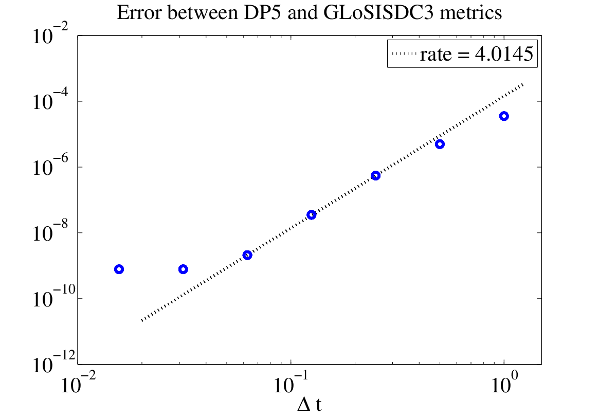
To verify temporal convergence, we first construct an accurate reference solution obtained by evolving the perturbed-black-hole initial data to final time with an explicit Dormand Prince 5 (DP5) timestepper and timestep . The spatial domain is determined by a top spherical harmonic index and , and is divided into 8 equally spaced concentric shells, each with with radial collocation points. Next, for each in a sequence of increasingly smaller timesteps we perform an analogous IMEX evolution using the GLoSISDC3 timestepper, which is fourth order accurate. One complication involves boundary conditions: we must ensure that the choices for the explicit and IMEX evolutions are consistent. For both we have chosen a “frozen” condition, in which the incoming characteristic is fixed to its initial value, i.e. we freeze in Eq. (18) to its initial value.
We compute the error,
| (28) |
and plot it in Figure 5. For intermediate , we observe the predicted fourth-order convergence rate. We remark that all timesteps shown in Fig. 5, except the largest, correspond to from the standpoint of the model problem analyzed in Section III.1. However, we have encountered no stability issues with these short-time evolutions.

We test spatial convergence as follows. Our spatial domain, determined by and , is divided into 4 equally spaced concentric shells. For a fixed , we then evolve the perturbed-black-hole initial data for different number of radial collocation points in each shell. We compute the root-mean-square sum of all constraint violations (see Eq. (53) of Ref. [25] for the precise definition), and plot it in Fig. 6. The figure indicates that the solution is dominated by spatial error, and exhibits convergence with increased spatial resolution. A plot of the dimensionless constraint norm defined in Eq. (71) of [25] is qualitatively the same.
III.3 Treatment of constraint damping terms

As described in Sec. II.1, the generalized harmonic equations (1) are modified by constraint damping terms proportional to in Eq. (1b). These terms cause constraint violations to decay exponentially. Because these terms are stiff, they require attention when choosing the IMEX splitting, as we now demonstrate.
We perform runs similar to Fig. 1 but for explicit () and implicit () constraint damping. The computational domain is the same as in Fig. 1 but with Cartesian center , , and . Our final evolution time for these runs is short enough that the weak instabilities (associated with small GLoSISDC3 timesteps) observed in Fig. 1 do not arise. Figure 7 shows the constraints for various timesteps and three different IMEX timesteppers. From the lowest panel, we see that the system is well-behaved for all considered timesteps if the constraint-damping terms are treated implicitly. The upper two panels show that for explicit handling of the constraint damping terms, the timestep matters: For small , the simulations behave well, for large they blow up. This is consistent with a Courant limit for the explicit sector of the timestepper, arising from the constraint-damping term.
III.4 Adaptive timestepping and comparison to explicit timestepper

In this subsection, we demonstrate adaptive timestepping in an IMEX evolution by using an adaptive timestepper on the perturbed-black-hole initial data from Appendix C. We evolved this initial data on a set of 16 concentric spherical shells with Cartesian center (0,0,0) and with , , and . A gravitational-wave pulse falls into a nonspinning black hole of mass shortly after , which causes a time-dependent deformation of the hole’s horizon. The top panel of Fig. 8 shows the minimum and maximum values of the intrinsic scalar curvature of the horizon: As the wave falls into the hole, the horizon shape oscillates and then relaxes back to the Schwarzschild value , which holds for the curvature of a sphere of Schwarzschild radius .
The bottom panel of Fig. 8 plots the step size chosen by the adaptive timestepper for an IMEX evolution and an analogous explicit evolution of the same initial data. The explicit timestepper chooses an essentially constant , right at its CFL stability limit. During the initial perturbation, the IMEX step size decreases to a local minimum; as the hole relaxes to its final time-independent configuration, the step size increases, eventually reaching an artificially imposed upper limit. (This upper limit was chosen to guarantee that the elliptic solver would converge in a reasonable amount of wallclock time.)
During the initial time-dependent perturbation, the IMEX evolution is usually able to take significantly larger timesteps than the analogous explicit evolution. In the explicit evolution, the Courant factor is limited to , which is comparable to the minimum of the IMEX evolution’s Courant factor.
We remark that the above IMEX simulations exhibit some instability: the IMEX run shows slow constraint growth, perhaps because we did not impose a constraint-preserving boundary condition on the outer boundary. However, the analogous explicit evolution exhibits no instability, and the IMEX and explicit evolutions’ constraint violations are comparable in size when we terminate the simulations (after time , which is long after the spacetime has relaxed to its final, stationary state).
IV Discussion
IV.1 Results obtained in the present work
In this article, we have further developed IMEX-techniques applied to hyperbolic systems. Specifically, we have moved beyond the model problem of a scalar wave [24] to the study of the full non-linear Einstein’s equations for single black hole spacetimes. Many results of the model problem presented in [24] carry over to Einstein’s equations in generalized harmonic form [25]: We continue to rewrite the implicit equation in second order form to utilize an existing elliptic solver [30]. Furthermore, as in the scalar-field case, we do not impose a boundary condition at the excision boundary inside the black hole. Uniqueness of the solution of the second order implicit equation is enforced, we believe, by the demand that the solution be regular across the horizon.
In contrast to the model problem, the generalized harmonic evolution system contains physical constraints11 1 These are in addition to the auxiliary constraints arising from the reduction to first order form. which in explicit simulations are handled with constraint damping [26, 7, 25]. We have introduced analogous constraint damping terms in the IMEX formulation, namely the terms proportional to in Eqs. (10) and (11). We have found that these constraint damping terms are essential for stability. Treating the constraint damping terms explicitly incurs a Courant limit due to their stiffness, and so we recommend an implicit treatment of these terms ().
We have focused our investigation on spectral deferred correction schemes [17, 18, 19, 20], utilizing 3 Gauss-Lobatto and 2 Gauss-Radau-right quadrature points: GLoSISDC3 and GRrSISDC2, respectively. These schemes generally work well; however, we find a weak instability for small timesteps which may be related to the stability region of the implicit sector of these IMEX schemes. We also have investigated ImexEuler and third order Additive Runge Kutta (ARK3). While ImexEuler proved robustly stable, our simulations with ARK3 showed a linear growing instability. The origin of this instability remains an open question.
The most demanding scenario that we have considered is a perturbed single black hole that rings down to a quiescent state. We have evolved this configuration with explicit and IMEX techniques. The explicit evolution used a fifth order Dormand-Prince timestepper with adaptive timestepping; however, because of the necessarily small grid-spacing close to the black hole, the explicit simulation uses an essentially constant timestep at its Courant limit, cf. Fig. 8. The IMEX method uses a small timestep for the early, dynamic part of the simulation, and then chooses increasingly larger timesteps, until it exceeds the explicit timestep by about a factor of 200.
For very large timesteps, the convergence rate of our elliptic solver deteriorates, and overall efficiency drops. Therefore, so far we have limited the IMEX timestep to times the explicit timestep. For these timesteps, the computational efficiency of the implicit and explicit code are approximately similar, for the example shown in Fig. 8. We are confident that improved preconditioning will accelerate convergence of the implicit solver, allowing us to utilize yet larger timesteps in IMEX at lower computational cost. Besides improved preconditioning, several aspects of our future work will increase the efficiency of the IMEX code: We plan to implement a more accurate starting method for the prediction phase of an SISDC timestep. We further plan to perform a detailed analysis of the required tolerances in the implicit solve (in the present work we set tolerances near numerical round-off to eliminate spurious instabilities due to insufficient accuracy), and we plan to optimize the C++ code implementing Eq. (17). We expect these steps to significantly increase efficiency of the IMEX code; in contrast, the explicit code is already highly optimized. In the next subsection, we discuss additional code improvements relevant to IMEX evolutions of binary black holes.
IV.2 Prospects for binary black hole evolutions
Long and accurate binary black hole simulations are needed for optimal signal-processing of current and future gravitational wave-detectors [10, 11, 12, 13]; this provides the motivation for the present work. While the results obtained here are very encouraging, additional work will be necessary to apply IMEX to black hole binaries.
First, the formalism must be adopted to the dual-frame approach [31] used in binary black hole simulations with SpEC. The corotating coordinates implemented via the dual-frame technique are essential for implicit time-stepping, because they localize the black holes in the computational coordinates. Without corotating coordinates, the black holes would move across the grid, resulting in rapid time-variability of the solution (on timescales , where denotes the velocity of the black hole with mass ). This variability would necessitate a small time-step to achieve small time-discretization error. The dual-frame technique merely adds a new advection term into the evolution equations, therefore, we expect the extension to dual-frames to be straightforward.
Second, the implicit solver must remain efficient despite the more complicated computational domain. And third, good outer boundary conditions will be necessary. We expect that the second and third issues can be addressed simultaneously with the following ideas: SpEC evolves binary black holes on a domain decomposition consisting of “inner” spherical shells around each of the black holes, which are surrounded by a complicated structure of “outer” subdomains (cylinders, distorted blocks and spherical shells, the latter of which extend to a large outer radius). The inner spherical shells require the highest resolution and therefore determine the Courant condition for fully explicit evolutions.
To simulate binary black holes with IMEX methods, we envision a split-by-region approach [32], where the inner spherical shells are treated with the IMEX techniques described in this paper and the outer subdomains are handled explicitly. The split-by-region approach has two important advantages: First, implicit equations will have to be solved only on series of concentric shells. This is the case considered here, for which SpEC’s elliptic solver is already reasonably efficient with further possible efficiency improvements as discussed in Sec. IV.1. In contrast, solution of implicit equations on the entire (rather complicated) domain-decomposition would likely be less efficient because of difficulties in preconditioning the inter-subdomain boundary conditions. Second, for explicit evolutions non-reflecting and constraint-preserving outer boundary conditions are available [25, 33, 34]. Explicit treatment of the region near the outer boundary will allow us to reuse these boundary conditions. In contrast, similarly sophisticated boundary conditions have not yet been investigated in an IMEX setting.
Because the outer subdomains will be handled explicitly, the split-by-region scheme will still be subject to a Courant condition, based on the minimum grid-spacing in the explicitly evolved region. Because the minimum grid-spacing in the outer subdomains is larger than the minimum grid-spacing near the black holes, the envisioned split-by-region approach should allow for timesteps larger by a factor
| (29) |
We shall assume that the cost-per-timestep is proportional to the number of collocation points, with different constants for explicit and IMEX cases:
| (30) | ||||
| (31) |
Here, is the ratio of the cost of an IMEX-timestep to a fully explicit timestep. The simulations presented in Sec. III give , with being somewhat larger for very large and somewhat smaller for small .
For temporal integration to a fixed final time, the number of timesteps for a fully explicit scheme will be proportional to , whereas for the IMEX split-by-region scheme, the number of timesteps will be proportional to . Therefore, the IMEX split-by-region scheme should require the following fractional amount of CPU resources relative to a completely explicit evolution (a smaller number indicates advantage for IMEX):
| (32) |
When , this simplifies to
| (33) |
As expected, the question is whether the larger timestep, encoded in , can compensate for the additional cost per timestep, encoded in . However, split-by-region mitigates the effect of by an extra factor .
To make this discussion concrete, a recent mass-ratio simulation of non-spinning black holes used , , and . With these values Eq. (33) gives , i.e. an IMEX evolution should be marginally more expensive than a fully explicit one. As the mass-ratio is further increased, the grid-spacing needed to resolve the smaller black hole decreases proportionally. Therefore, will decrease proportional to , and will increase proportional to . The constant of proportionality can be determined from at , so that . The number of grid-points will only modestly change, so we assume . Then from Eq. (33) we estimate an efficiency increase for IMEX of
| (34) |
Therefore, with increasing mass-ratio, IMEX will become increasingly more efficient than the explicit evolution code.
The additional efficiency gains for IMEX discussed in Sec. IV.1 are not taken into account in this estimate. Furthermore, a more judicious choice of domain decomposition with a more carefully tuned number of collocation points in the inner spheres would reduce the ratio . Finally, we have not accounted for the fact that BBH evolutions require additional CPU resources for interpolation. Because interpolation occurs only in the outer subdomains, this will reduce .
On the other hand, at this point we do not know how accurately the implicit equations must be solved in the binary case; if higher accuracy is required to control secularly accumulating phase-errors, then each implicit solve would become more expensive. Furthermore, the binary simulations utilize a dual-frame method which will add some overhead to the implicit solutions.
In summary, we believe that IMEX schemes offer the promise of faster binary black-hole simulations, but many interesting issues (such as those outlined in this section) deserve further investigation.
IV.3 Applicability to other computational techniques
The results in this paper were obtained for the generalized harmonic formulation of Einstein’s equations using pseudo-spectral methods. IMEX methods might also be implemented for other formulations of the Einstein equations, such as the Baumgarte-Shapiro-Shibata-Nakamura (BSSN) formulation [35, 36] or the recent conformal decompositions of the Z4 formulation [37]. Indeed, for such systems specification of the first-order implicit system [analogous to Eqs. (10)] corresponding to a single time-step is straightforward. However, relative to the analogous reduction performed for the generalized harmonic formulation in this paper, the reduction of such a first-order system to a second-order system involving, presumably, some subset of the system variables would seem to be more involved. A second impediment arises from the need to use corotating coordinates. In corotating coordinates, temporal timescales are long, allowing large time-steps with sufficiently small time-discretization error (cf. Sec. IV.2). To our knowledge, none of the BSSN/Z4 codes currently utilize corotating coordinates, although, in principle, the dual-frame approach [31] could be applied in such codes.
Provided the existence of efficient solvers for the resulting discretized implicit equations, the IMEX methods developed here should also be applicable to other spatial discretizations, e.g. finite differences, finite elements, or other Galerkin spectral-element approaches. The presence of a horizon and the replacement of an inner boundary condition by a regularity condition (cf. Sec. II.3) are points demanding particular attention. In our approach each component of the apparent horizon is covered by a single subdomain. Therefore, in our pseudo-spectral treatment the metric in the vicinity of the horizon is expanded in terms of a single set of basis functions, with regularity of the solution an automatic consequence. Guaranteed regularity of the solution might be lost for either a finite-difference method or an unstructured-mesh method, but further studies of these possibilities are clearly warranted.
Acknowledgements.
We are pleased to thank Saul Teukolsky, Larry Kidder, Jan Hesthaven, and Mike Minion for helpful discussions. This work was supported in part by the Sherman Fairchild foundation, NSF grants Nos. PHY-0969111 and PHY-1005426, and NASA grant No. NNX09AF96G at Cornell; and by NSF grant No. PHY 0855678 to the University of New Mexico. H.P. gratefully acknowledges support from the NSERC of Canada, from the Canada Research Chairs Program, and from the Canadian Institute for Advanced Research. Some computations in this paper were performed using the GPC supercomputer at the SciNet HPC Consortium; SciNet is funded by: the Canada Foundation for Innovation under the auspices of Compute Canada; the Government of Ontario; Ontario Research Fund — Research Excellence; and the University of Toronto. Some computations in this paper were performed using Pequena at the UNM Center for Advanced Research Computing.Appendix A Decomposition of
The trace of the Christoffel symbol of the first kind is
| (35) |
Writing the time-derivative separately, we reach
| (36) |
where is the time component. Now we insert the identities and , thereby finding
| (37) |
Finally, we use the identity to write
| (38) |
Using the last expression, we compute
| (39a) | ||||
| (39b) | ||||
and these formulas complete the definitions in Eqs. (11).
Appendix B Semi-implicit spectral deferred corrections
This appendix describes one of the IMEX timestepping algorithm used for our evolutions, summarizing results found in Refs. [17, 18, 19, 20] and expressing them in our notation. We aim here only to describe the algorithm, and do not address stability and convergence issues (which have been exhaustively explored in the references).
B.1 Collocation approximation of the Picard integral
We start with the generic ODE initial value problem Eq. (4). Each spectral deferred correction method specifies a rule for advancing the vector at the present timestep (perhaps the initial time ) to a vector at the next timestep . The Picard integral form of the initial value problem Eq. (4) for starting value is
| (40) |
We consider this equation on the interval , and show how iterative approximation of (40) yields a timestepping scheme.
Introduce collocation nodes which are also time sub-steps:
| (41) |
The are either Gauss-Legendre, Gauss-Lobatto, or Gauss-Radau nodes relative to the standard interval . Each of the endpoints, and , may or may not be a collocation node. In particular, for the Gauss-Legendre case both and are not in .
Define a system vector at each collocation point . A solution to the polynomial collocation approximation to the Picard integral (40) is a set of vectors obeying
| (42) | ||||
where is the unique degree (vector-valued) polynomial which interpolates the data
| (43) |
The elements define the spectral integration matrix. The solution to Eq. (42) defines the approximation
| (44) |
We get an approximation to the solution of the collocation equations (42) via an iteration described below (that is, we get an approximate solution to the approximating system of equations).
B.2 Iterative solution of the collocation equations
Our iterative scheme for solving (42) relies on two phases: (i) an initial prediction phase which generates a provisional solution , and (ii) a correction phase which generates successive improvements , as described in detail below. As described by Hagstrom and Zhou [20], the prediction phase requires a starting method, and we use ImexEuler. For each the set determines an interpolating polynomial , and the numerically computed approximation to is
| (45) |
For the Gauss-Legendre, Gauss-Radau-right, and Gauss-Lobatto cases, Hagstrom and Zhou [20] have studied the accuracy of these methods. When considered as global methods (integration to a fixed time with multiple timesteps), they have shown that for sufficiently large the optimal order of attainable accuracy is respectively , , and , that is the same order as for the underlying quadrature rule; however, this order is typically not obtained for the vectors at intermediate times.
Typically for Gauss-Legendre, for Gauss-Radau (left or right), and for Gauss-Lobatto cases, where each choice should yield the optimal order of accuracy. Our presentation of the iteration algorithm makes use of the notations
| (46) | ||||
but draws a distinction between two cases (i) Gauss-Legendre and Gauss-Radau-right (for these methods is not a collocation point) and (ii) Gauss-Lobatto and Gauss-Radau-left (for these is a collocation point).
To start the prediction phase for Gauss-Legendre and Gauss-Radau-right, we first solve
| (47) |
to get . For Gauss-Lobatto or Gauss-Radau-left, we have to start with. We then march forward in time by solving in sequence the following equations:
| (48) |
for . Note that each such equation is defined by the previously constructed and amounts to an ImexEuler timestep.
We have used ImexEuler to generate the provisional solution , and this simple method is also the basis of the correction phase. Given , a correction sweep yields updated vectors. . To understand the eventual scheme which produces the updated vectors, first consider an approximate solution to the continuum initial value problem Eq. (4), assuming , along with the residual
| (49) |
If the exact solution is , then the correction obeys
| (50) |
We timestep this equation using ImexEuler. For case (i), either Gauss-Legendre or Gauss-Radau-right, we first solve
| (51) | ||||
for , where to reach this equation we have used . For the case (ii) methods we have to start with. Subsequently, we solve
| (52) | ||||
for .
To exploit formulas (51)–(52), first make the assignments
| (53) | ||||
With these assignments in Eq. (51), we find, upon adding to both sides of the equation,
| (54) | ||||
Solution of this equation yields . Notice that its right-hand side is determined by the known vectors . Next, with the assignments (53) in (52), we find, upon adding to both sides,
| (55) | ||||
where we have defined the shorthand
| (56) |
Sequential solution of this tower of equations yields for .
As mentioned, for any method [Gauss-Legendre, Gauss-Radau (left or right), Gauss-Lobatto] Eq. (45) defines a numerical computed approximation to ; however, note that for Gauss-Lobatto and Gauss-Radau-right, we may also use for this approximation, since for these cases.
Appendix C Perturbed Kerr Initial-Data
In Sec. III we use initial data representing a nonspinning Kerr black hole with a superposed gravitational wave. Initial data sets are constructed following the method of [38], which is based on the extended conformal thin sandwich (XCTS) formalism. The Einstein constraint equations read [39, 40]
| (57) | ||||
| (58) |
where is the covariant derivative compatible with the spatial metric , is the trace of the Ricci tensor of , and is the trace of the extrinsic curvature of the initial data hypersurface.
The conformal metric and conformal factor are defined by
| (59) |
and the time derivative of the conformal metric is denoted by
| (60) |
which satisfies . The conformal lapse is given by . Applying this conformal decomposition, Eqs. (57)–(58) can be written as
| (61) | |||
| (62) |
and the evolution equation for yields the following equation for the lapse:
| (63) |
Here , is the covariant derivative compatible with , is the trace of the Ricci tensor of , and , which is related to by
| (64) |
For given , , , and , Eqs. (61), (62), and (63) are a coupled set of elliptic equations that can be solved for , , and . From these solutions, the physical initial data and are obtained from (59) and (64), respectively.
To construct initial data describing a Kerr black hole initially in equilibrium, together with an ingoing pulse of gravitational waves, we make the following choices for the free data,
| (65) | ||||
| (66) | ||||
| (67) | ||||
| (68) |
In the above, and are the spatial metric and the trace of the extrinsic curvature in Kerr-Schild coordinates, with mass parameter and spin parameter . The pulse of gravitational waves is denoted by and is chosen to be an ingoing, even parity, , linearized quadrupole wave as given by Teukolsky [41, 42]). The explicit expression for the spacetime metric of the waves in spherical coordinates is
| (69) |
where the radial functions are
| (70) | ||||
| (71) | ||||
| (72) |
and the shape of the waves is determined by
| (73) | ||||
| (74) |
We choose to be a Gaussian with width at initial radius . The constant in Eq. (65) is the amplitude of the waves. We use the value .
References
- [1] B. C. Barish and R. Weiss, Phys. Today 52, 44 (1999).
- [2] D. Sigg and the LIGO Scientific Collaboration, Class. Quantum Grav. 25, 114041 (2008).
- [3] F. Acernese et al., Class. Quantum Grav. 25, 184001 (2008).
- [4] K. Kuroda and the LCGT Collaboration, Class. Quantum Grav. 27, 084004 (2010).
- [5] T. Prince et al., LISA: Probing the Universe with Gravitational Waves, Tech. Rep. (LISA science case document, 2009) revised version available at http://list.caltech.edu/mission_documents.
- [6] O. Jennrich, Class. Quantum Grav. 26, 153001 (2009).
- [7] F. Pretorius, Phys. Rev. Lett. 95, 121101 (2005).
- [8] J. Centrella, J. G. Baker, B. J. Kelly, and J. R. van Meter, Rev. Mod. Phys. 82, 3069 (2010).
- [9] L. Santamaría, F. Ohme, P. Ajith, B. Brügmann, N. Dorband, M. Hannam, S. Husa, P. Mösta, D. Pollney, C. Reisswig, E. L. Robinson, J. Seiler, and B. Krishnan, Phys. Rev. D 82, 064016 (2010).
- [10] M. Hannam, S. Husa, F. Ohme, and P. Ajith, Phys. Rev. D 82, 124052 (2010).
- [11] T. Damour, A. Nagar, and M. Trias, Phys. Rev. D 83, 024006 (2011).
- [12] I. MacDonald, S. Nissanke, and H. P. Pfeiffer, Class. Quantum Grav. 28, 134002 (2011), arXiv:1102.5128 [gr-qc] .
- [13] M. Boyle, Phys. Rev. D 84 (2011).
- [14] C. O. Lousto and Y. Zlochower, Phys. Rev. Lett. 106, 041101 (2011).
- [15] U. Sperhake, V. Cardoso, C. D. Ott, E. Schnetter, and H. Witek, (2011), arXiv:1105.5391 [gr-qc] .
- [16] G. Lovelace, M. A. Scheel, and B. Szilágyi, Phys. Rev. D 83, 024010 (2011).
- [17] A. Dutt, L. Greengard, and V. Rokhlin, BIT 40, 241 (2000).
- [18] M. L. Minion, Commun. Math. Sci. 1, 471 (2003).
- [19] A. T. Layton and M. L. Minion, BIT 45, 341 (2005).
- [20] T. Hagstrom and R. Zhou, Commun. App. Math. and Comp. Sci. 1, 169 (2006).
- [21] A. van Zuijlen, A. de Boer, and H. Bijl, J. Comput. Phys. 224, 414 (2007).
- [22] C. Palenzuela, L. Lehner, O. Reula, and L. Rezzolla, Mon. Not. Roy. Astr. Soc. 394, 1727 (2009).
- [23] S. Y. Kadioglu and D. A. Knoll, J. Comput. Phys. 229, 3237 (2010).
- [24] S. R. Lau, H. P. Pfeiffer, and J. S. Hesthaven, Commun. Comput. Phys. 6, 1063 (2009).
- [25] L. Lindblom, M. A. Scheel, L. E. Kidder, R. Owen, and O. Rinne, Class. Quantum Grav. 23, S447 (2006).
- [26] C. Gundlach, J. M. Martin-Garcia, G. Calabrese, and I. Hinder, Class. Quantum Grav. 22, 3767 (2005).
- [27] M. Holst, L. Lindblom, R. Owen, H. P. Pfeiffer, M. A. Scheel, and L. E. Kidder, Phys. Rev. D 70, 084017 (2004).
- [28] C. A. Kennedy and M. H. Carpenter, Appl. Numer. Math. 44, 139 (2003).
- [29] N. W. Taylor, L. E. Kidder, and S. A. Teukolsky, Phys. Rev. D82, 024037 (2010), arXiv:1005.2922 [gr-qc] .
- [30] H. P. Pfeiffer, L. E. Kidder, M. A. Scheel, and S. A. Teukolsky, Comput. Phys. Commun. 152, 253 (2003).
- [31] M. A. Scheel, H. P. Pfeiffer, L. Lindblom, L. E. Kidder, O. Rinne, and S. A. Teukolsky, Phys. Rev. D 74, 104006 (2006).
- [32] A. Kanevsky, M. H. Carpenter, D. Gottlieb, and J. S. Hesthaven, J. Comput. Phys. 225, 1753 (2007).
- [33] O. Rinne, L. Lindblom, and M. A. Scheel, Class. Quantum Grav. 24, 4053 (2007).
- [34] O. Rinne, L. T. Buchman, M. A. Scheel, and H. P. Pfeiffer, Class. Quantum Grav. 26, 075009 (2009).
- [35] M. Shibata and T. Nakamura, Phys. Rev. D 52, 5428 (1995).
- [36] T. W. Baumgarte and S. L. Shapiro, Phys. Rev. D 59, 024007 (1998), gr-qc/9810065.
- [37] D. Alic, C. Bona-Casas, C. Bona, L. Rezzolla, and C. Palenzuela, (2011), arXiv:1106.2254 [gr-qc] .
- [38] H. P. Pfeiffer, L. E. Kidder, M. A. Scheel, and D. Shoemaker, Phys. Rev. D 71, 024020 (2005).
- [39] H. P. Pfeiffer, J. Hyperbol. Differ. Eq. 2, 497 (2005).
- [40] G. Cook, Living Rev. Rel. 3 (2000), 5.
- [41] S. A. Teukolsky, Phys. Rev. D 26, 745 (1982).
- [42] O. Rinne, Class. Quantum Grav. 26, 048003 (2009).