An Algorithmic Solution to the Five-Point Pose Problem Based on the Cayley Representation of Rotations
Abstract.
We give a new algorithmic solution to the well-known five-point relative pose problem. Our approach does not deal with the famous cubic constraint on an essential matrix. Instead, we use the Cayley representation of rotations in order to obtain a polynomial system from epipolar constraints. Solving that system, we directly get relative rotation and translation parameters of the cameras in terms of roots of a 10th degree polynomial.
Key words and phrases:
Five-point pose problem, epipolar constraints, Cayley representation1. Introduction
In the paper presented we give an algorithmic solution to the 5-point 2-view relative pose problem. It is formulated as follows.
Problem 1.
We are given two calibrated pinhole cameras with centers , and five points lying in front of the cameras in 3-dimensional Euclidean space, see Figure 1. In every camera coordinate frame the directing vectors of are only known. The problem is in finding the relative position and orientation of the second camera with respect to the first one.
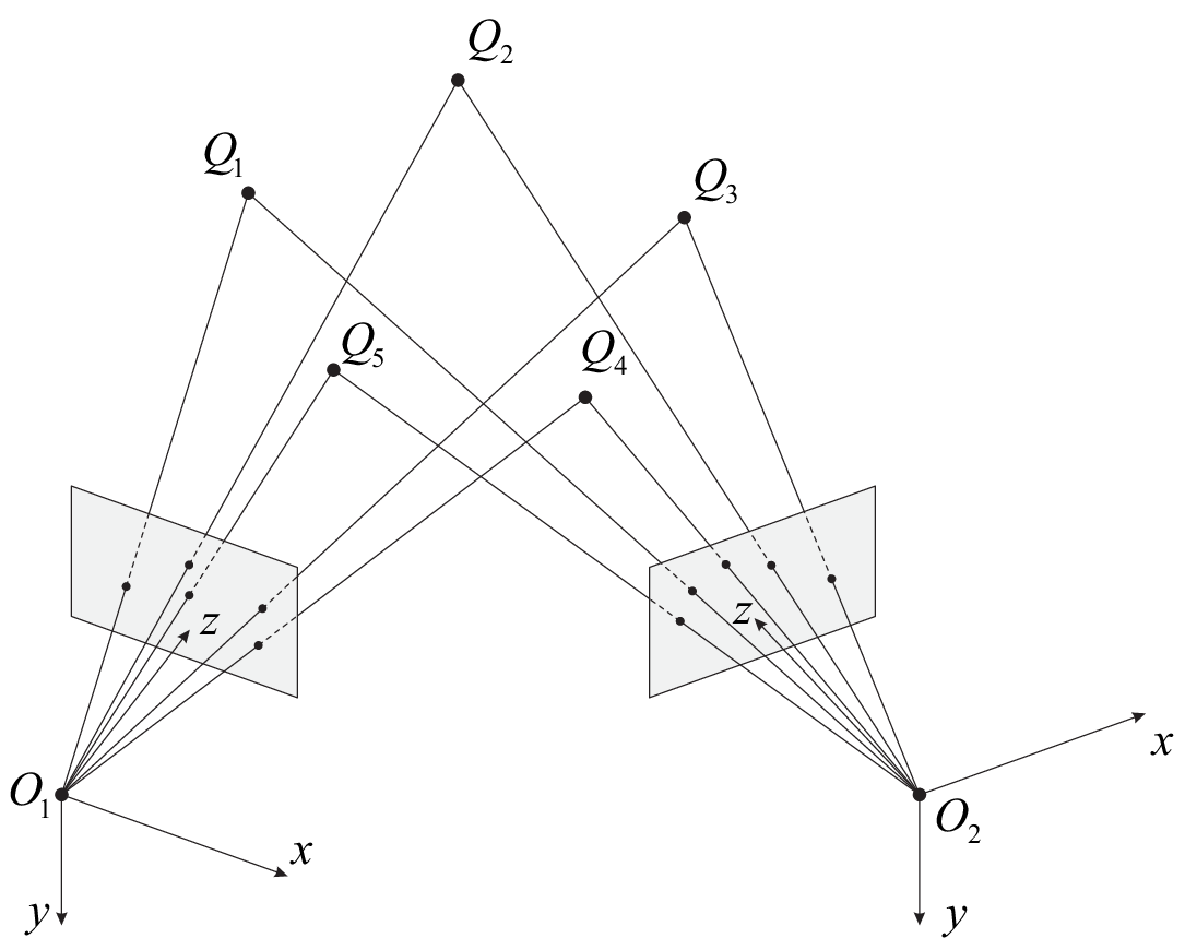
The 5-point relative pose problem is a key to the 3d scene reconstruction problem, which is in turn used in many computer vision applications such as augmented reality, self-parking systems, robot path-planning, navigation, etc. It is well known that 5-point algorithms yield significantly better results in accuracy and reliability than 6-, 7- and 8-point algorithms. Moreover, for planar and near-planar scenes only 5-point method allows to get a robust solution without any additional modification of the algorithm.
Problem 1 was first shown by Kruppa [8] in 1913 to have at most eleven solutions. Using the methods of projective geometry, he proposed an algorithm for solving the problem, although it could not lead to a numerical implementation. Demazure [2], Faugeras and Maybank [4], Heyden and Sparr [6] then sharpened Kruppa’s result and proved that the exact number of solutions (including complex) is ten.
More efficient and practical solution has been presented by Philip [13] in 1996. His method requires to solve a 13th degree polynomial. In 2004 Nistér [12] improved Philip’s algorithm and expressed a solution in terms of a real root of 10th degree polynomial. Afterwards, there were presented many modifications of that algorithm simplifying its implementation [10] or making it more numerically stable [9, 15].
In this paper we give yet another algorithmic solution to the problem using the well-known Cayley representation of rotation matrices [1]. Our approach does not mix rotation and translation parameters of an essential matrix and nevertheless allows one to express a solution in terms of a root of 10th degree univariate polynomial. Experiments on synthetic data show that the method is comparable in accuracy with the existing five-point solvers.
The rest of the paper is organized as follows. In Section 2 we describe in detail our algorithm. In Section 3 we make a comparison of our algorithm with the original Nistér solver [12] on synthetic data. Section 4 concludes.
1.1. Notation
We use for column vectors, and for matrices. For a matrix , the entries are , the transpose is , the trace is , and the determinant is . For two vectors and , the vector product is , and the scalar product is . For a vector , the notation stands for a skew-symmetric matrix such that for any vector .
We use for identical matrix and for zero matrix or vector, for the Frobenius norm.
2. Description of the algorithm
2.1. Initial data transformation
Initial data for our algorithm are the homogeneous coordinates , , of points in the coordinate frame of th camera, , (see Figure 1).
Without loss of generality we can set for . The numerically stable way of doing this is as follows. We combine the initial data into two matrices
| (1) |
and compute the matrices
| (2) |
where and are the Householder matrices zeroing , and respectively. The corresponding Householder vectors are
2.2. Epipolar constraints and essential matrix
We first recall some definitions from multiview geometry, see [3, 5, 11] for details. A pinhole camera is a triple , where is an image plane, is a central projection of points in 3-dimensional Euclidean space onto , and is a camera center (center of projection ). The focal length is the distance between and , the orthogonal projection of onto is called the principal point. A pinhole camera is called calibrated if all its intrinsic parameters (such as focal length and principal point’s coordinates) are known.
Let there be given two calibrated pinhole cameras , . Without loss of generality we can set , , where is the rotation matrix and is the translation vector normalized so that .
2.3. Ten fourth degree polynomials
Our approach is based on the following well-known result.
Theorem 1 ([1]).
If a matrix is not a rotation through the angle , , about certain axis, then can be represented as
| (4) |
where .
Let be represented by (4) and be an essential matrix.
Proposition 1.
If
| (5) |
where , then .
Proof.
Consider a matrix , where the Householder matrix . Then, . By a straightforward computation, the equation has a unique solution (5). ∎
Since epipolar constraints (3) are linear and homogeneous in , we can rewrite them as
| (6) |
where the th row of matrix is
Now we represent rotation in form (4) and take the determinants of all submatrices of matrix . This yields ten polynomial equations:
| (7) |
where , means a polynomial of degree in the variable , is a constant.
Remark 1.
Actually, the determinants of submatrices of give the following expressions:
where and is a polynomial of 6th total degree. However, one can verify that is factorized as and the coefficients of are easily deduced from the coefficients of .
2.4. Tenth degree univariate polynomial
We expand system (8) with 20 more polynomials , for , and for . Thus we get
| (9) |
where is a new coefficient matrix and
is the five-degree monomial vector. It is clear that system (9) is equivalent to (8).
We rearrange columns of matrix and perform Gauss-Jordan elimination with partial pivoting on it. Then the last six rows of the resulting matrix can be represented in form
,
where empty spaces are occupied by zeroes. Also, we have omitted first 28 zero columns. From the corresponding six polynomials we obtain the following four polynomials
| (10) |
where matrix can be represented as
| (11) |
Remark 2.
Since we use only six last rows of matrix , there is no need to perform a “complete” Gauss-Jordan elimination on matrix . For the first 24 rows of only lower triangular entries should be zeroed.
Denote by . In general, it is a 20th degree polynomial in .
Proposition 2.
Polynomial has a special symmetric form:
| (12) |
where .
Proof.
Due to the conditions , we have . As a consequence,
Substituting this into the last identity in (5), we get . Thus, if is a root of , then so is . It follows that
∎
Substituting , we transform to a 10th degree polynomial
| (13) |
where can be deduced using the formula . The result reads
| (14) |
where the primed sum is taken over all from to 10 such that . Note that in case the r.h.s. of (14) becomes .
2.5. Structure recovery
A complex root of leads to a complex root of and by (4) to complex rotation matrix having no geometric interpretation. Hence only real roots of must be treated.
Real roots of can be efficiently found first using Sturm sequences [7] for isolating and then Ridders’ method [14] for polishing. Then we can recover the second camera matrix applying the following algorithm.
Let be a real root of . First we find the value
which is a root of subject to . After that, we obtain the - and -components of the solution by applying Gaussian elimination with partial pivoting on matrix in (11).
Then we find the entries of by (4). Given , the translation vector can be found by performing Gaussian elimination with partial pivoting on matrix in (6). Here we have also taken into account the normalization constraint .
Let and . It is well-known [5, 12] that there are four possibilities for the second camera matrix: , , and . The only of these matrices is correct, all others correspond to unfeasible configurations.
The true second camera matrix can be derived from the so-called cheirality constraint saying that all the scene points must be in front of the cameras. In particular, this is valid for the first scene point . Denote by
| (15) |
Then,
- •
if and , then ;
- •
else if and , then ;
- •
else if and , then ;
- •
else .
Here the value and are computed in the same manner as and in (15) with being replaced by .
Finally, the initial second camera matrix is given by
where the Householder matrices and are defined in Subsection 2.1.
3. Experiments on synthetic data


In this section we compare our algorithm with the original 5-point solver by Nistér [12] on synthetic data. The C/C++ implementations of both algorithms have been written. All computations are performed in double precision. Synthetic data setup is the same as in [12]:
| Distance to the scene | 1 |
|---|---|
| Scene depth | 0.5 |
| Baseline length | 0.1 |
| Image dimensions | |
| Field of view | 45 degrees |
The numerical error is defined by
| (16) |
where is the ground truth second camera matrix.
The numerical error distributions are reported in Figure 2. The total number of trials is in each experiment. We have compared the algorithms first in case of default conditions (Figure 2(a)) and second in the most problematic case in sense of numerical stability — planar scene and forward motion (Figure 2(b)).
In Figure 3 we demonstrate the behaviour of the algorithms under increasing image noise. We add the Gaussian noise with a standard deviation varying from 0 to 1 pixel in a image. One sees that in presence of noise the results of both algorithms are almost coincident.


4. Discussion of results
A new algorithm for the 5-point relative pose problem is presented. A computation on synthetic data confirms that it is robust enough. In whole, it is a good alternative to the existing five-point solvers. Its major advantage is that it yields a direct structure recovery, i.e. a reconstruction without computing an essential matrix. Such approach is more flexible when we are given some additional information on the camera rotations and/or translations. For instance, if the Euler angles , representing matrix , are known to lie in some limits, then so is the variable
| (17) |
This allows one to discard some roots of the 10th degree polynomial at once without structure recovery step.
References
- [1] Cayley, A.: Sur Quelques Propriétés des Déterminants Gauches. J. Reine Angew. Math. 32, 119-123 (1846).
- [2] Demazure, M.: Sur Deux Problemes de Reconstruction. Technical Report No 882, INRIA (1988).
- [3] Faugeras, O.: Three-Dimensional Computer Vision: A Geometric Viewpoint. MIT Press (1993).
- [4] Faugeras, O., Maybank, S.: Motion from Point Matches: Multiplicity of Solutions. International Journal of Computer Vision 4, 225-246 (1990).
- [5] Hartley, R., Zisserman, A.: Multiple View Geometry in Computer Vision. Second Edition. Cambridge University Press (2004).
- [6] Heyden, A., Sparr, G.: Reconstruction from Calibrated Camera – A New Proof of the Kruppa-Demazure Theorem. Journal of Mathematical Imaging and Vision 10, 1-20 (1999).
- [7] Hook, D.G., McAree, P.R.: Using Sturm Sequences To Bracket Real Roots of Polynomial Equations. Graphic Gems I. Academic Press, 416-422 (1990).
- [8] Kruppa, E.: Zur Ermittlung eines Objektes aus zwei Perspektiven mit Innerer Orientierung. Sitz.-Ber. Akad. Wiss., Wien, Math. Naturw. Kl. Abt. 122, 1939-1948 (1913).
- [9] Kukelova, Z., Bujnak, M., Pajdla, T.: Polynomial eigenvalue solutions to the 5-pt and 6-pt relative pose problems. British Machine Vision Conference (2008).
- [10] Li, H., Hartley, R.: Five-Point Motion Estimation Made Easy. IEEE-ICPR, 630-633 (2006).
- [11] Maybank, S.: Theory of Reconstruction from Image Motion. Springer-Verlag (1993).
- [12] Nistér, D.: An Efficient Solution to the Five-Point Relative Pose Problem. IEEE Transactions on Pattern Analysis and Machine Intelligence 26, 756-777 (2004).
- [13] Philip, J.: A Non-Iterative Algorithm for Determining all Essential Matrices Corresponding to Five Point Pairs. Photogrammetric Record 15, 589-599 (1996).
- [14] Press, W., Teukolsky, S., Vetterling, W., Flannery, B.: Numerical recipes in C, Cambridge University Press (1988).
- [15] Stewénius, H., Engels, C., Nistér, D.: Recent Developments on Direct Relative Orientation. ISPRS Journal of Photogrammetry and Remote Sensing 60, 284-294 (2006).