A Control-Oriented Notion of Finite State Approximation

We begin by establishing several facts that will help demonstrate the relevance of the proposed notion of approximation to the problem of certified-by-design controller synthesis.

As a consequence of these simple facts, if we were to partition each of $P$ and $\hat{P}_{i}$ into equivalence classes of feasible signals having identical first and third components (corresponding to control inputs and sensor outputs), the existence of a surjective map $\psi_{i}$ satisfying condition (a) of Definition 6 effectively establishes a 1-1 correspondence between the equivalence classes of $P$ and $\hat{P}_{i}$. Moreover, it follows from condition (b) of Definition 6 that if all signals in a given equivalence class of $\hat{P}_{i}$ satisfy a $\rho/\mu$ gain stability condition, then so do all the signals of the corresponding equivalence class of $P$. This is formalized and proved in the following statements.

We are now ready to turn our attention to the problem of control synthesis.

Theorem 1 implies that the original problem of designing a controller $K$ for the plant $P$ to meet performance objective (2) can be substituted by the problem of designing a controller $K$ for some $\hat{P}_{i}$ to meet an auxiliary performance objective (4), since any feedback controller that allows us to meet the closed loop specifications of the latter problem also allows us to meet the closed loop specifications of the former problem. Of course, the problem of finding a controller $K$ such that the feedback interconnection $(\hat{P}_{i},K)$ satisfies (4) is a difficult problem in general, since $\Delta_{i}$ can be an arbitrarily complex system. However, a simpler problem can be posed by utilizing the available characterization of the approximation error $\Delta_{i}$ in terms of $\rho_{\Delta}/\mu_{\Delta}$ gain stability with gain $\gamma_{i}$. Similar to what is done in the classical robust control setting, the idea is to design $K$ such that the interconnection of $\hat{M}_{i}$, $K$ and any $\Delta$ in the class $\mathbf{\Delta}_{i}$

satisfies the auxiliary performance objective (4). This synthesis problem can be elegantly formulated using the ‘Small Gain Theorem’ proposed in [17].

Interpreting Theorem 2 where “$S$” represents the feedback interconnection of $\hat{M}_{i}$ and $K$ and where “$\Delta$” represents the corresponding approximation error $\Delta_{i}$, we can formulate the following:

The problem of designing a controller $K$ for a DFM $\hat{M}_{i}$ so that the closed loop system satisfies a gain condition (such as (7)) can be systematically addressed by solving a corresponding discrete minimax problem. Interested readers are referred to [18] for the details of the approach.

Intuitively, the availability of such finite approximations allows one to successively replace the original synthesis problem by two problems: The first (Theorem 1) allows one to approximate the performance objectives when the exogenous input and performance output of the plant are not finite valued. The second (Theorem 3) allows one to simplify the synthesis problem at the expense of additional conservatism by introducing a set based description of the approximate model. In practice, exact computation of $\gamma_{i}$ may be computationally prohibitive if not impossible. Gain bounds are typically used, leading to a hierarchy of synthesis problems and controllers.

We conclude with a final observation:

Consider a tank with area $A$ (sq.cm.) and height $h$ (cm), a binary sensor that indicates whether the water level is above or below $h/2$, and an actuator that can pump water in or drain water out at a rate $p$ (liters/minute). The dynamics of the sampled plant $P$, from which we receive a measurement $y\in\mathcal{Y}=\{\textrm{`Empty'},\textrm{`Full'}\}$ at the beginning of every sampling instant and choose and hold a control input $u\in\mathcal{U}=\{\textrm{`Pump'},\textrm{`Drain'}\}$ until the next sampling instant, is given by

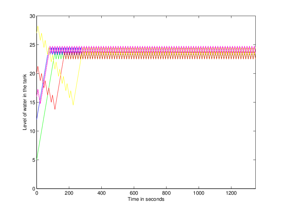
where $T$ is the sampling interval (seconds). Our objective is to drive and hold the water level within some desired bounds, in the absence of exogenous input $r$. The performance output $v$ is chosen to take the value $0$ when the water level falls within the desired bounds and $1$ otherwise. The performance objective can thus be written as a gain condition (2), with $\rho(r)=0$ and $\mu(v)=v$. Letting $A=100$, $h=30$, $p=1$, $T=7.5$, and choosing a desired water level between 22.5 and 25cm, the components of the $\rho/\mu$ approximation are constructed as follows: For $i=1$, the tank is first partitioned into $6$ equal intervals of length $h/6$, while for each subsequent $i$ the number of elements in the partition are doubled (i.e. $i=2\leftrightarrow 12$ elements, $i=3\leftrightarrow 24$ elements,…). The states of $\hat{M}_{i}$ are the elements of the partition as well as unions of arbitrary numbers of neighboring elements. $\hat{M}_{i}$ is initialized to the state encompassing the whole tank (reflecting our lack of knowledge of the plant’s initial state). The transitions of $\hat{M}_{i}$ are deterministic by construction, while its output $\hat{y}_{i}$ is not: Outputs associated with states corresponding to intervals crossing $h/2$ are interpreted as false predictions when computing the gain of the error system $\Delta_{i}$. Error system $\Delta_{i}$ has input $z=u$ and output $w\in\{0,1\}$, with $w=0$ ($w=1$) indicating a sensor output match (mismatch) between $P$ and $\hat{M}_{i}$. $\Delta_{i}$ is described by gain condition (6), where $\rho_{\Delta}(z)=\rho_{\Delta}(u)=1$ and $\mu_{\Delta}(w)=w$. Note that the construction is similar to that proposed in [18], but with a different gain condition describing the performance objectives as reachability specifications are considered here rather than exponential stability with guaranteed rate of convergence. The performance output $\hat{v}_{i}$ is set to $0$ for states lying entirely within the desired bounds, and set to $1$ otherwise.

Implementing this algorithm: For $i=1$ and $i=2$, the gain bound of $\Delta$ is 1, and design is not successful. For $i=3$, the gain bound is $0$: The approximate model thus succeeds in perfectly predicting the sensor output of the plant after some transient. Moreover, control design is successful: Representative paths of the water level in the closed loop system, consisting of the plant in feedback with the controller (a DFM with 190 states) are plotted in Figure 3 for various plant initial conditions. Of course, as design is successful, it is unecessary to construct the remaining components of the $\rho/\mu$ approximation sequence for $i\geq 4$.

In the classical setting, a stable LTI plant $\tilde{P}$ of order $m$ can be considered an approximation of a stable LTI plant $P$ of order $n>m$ if we can recover $P$ by perturbing $\tilde{P}$ using a small stable perturbation. The proposed notion has a similar flavor, with the caveat that we cannot generally hope to exactly recover the performance objective due to the finiteness of the input and output alphabets of a DFM. Alternatively, note that the notion of approximation proposed in Definition 6 has an interpretation in the classical setting (i.e. if we drop the requirements that $\hat{M}_{i}$ is a DFM and that $\mathcal{U}$, $\mathcal{Y}$ are finite). Indeed, assume that $P$ is a stable LTI system of order $n$ and each $\hat{M}_{i}$ is a stable LTI system of order $m_{i}\leq n$. In this case, $\hat{\mathcal{R}}_{i}=\mathcal{R}=\mathcal{U}=\mathcal{Z}$, $\hat{\mathcal{V}}_{i}=\mathcal{V}=\mathcal{Y}=\mathcal{W}$, $\Delta_{i}$ is a stable LTI system given by $\Delta_{i}=P-M_{i}$ and is an additive perturbation of $M_{i}$ as shown in Figure 4. Thus $\hat{P}_{i}=P$ and $\psi_{i}$ is simply the identity map. Intuitively, $\psi$ captures the necessity, in general, to approximate the performance objective in addition to the plant for the class of problems considered in this paper, unless the original plant $P$ is itself a DFM. Moreover, additional input and output channels are needed here (for $w$ and $z$) as signals cannot simply be added as in the LTI setting.

References

- [1] R. Alur, T. Henzinger, G. Lafferriere, and G. J. Pappas, “Discrete abstractions of hybrid systems,” Proceedings of the IEEE, vol. 88, no. 2, pp. 971–984, 2000.
- [2] C. Belta, A. Bicchi, M. Egerstedt, E. Frazzoli, E. Klavins, and G. J. Pappas, “Symbolic planning and control of robot motion: State of the art and grand challenges.” IEEE Robotics and Automation Magazine, vol. 14, no. 1, pp. 61–70, March 2007.
- [3] T. T. Georgiou and M. C. Smith, “Robustness analysis of nonlinear feedback systems: An input-output approach,” IEEE Transactions on Automatic Control, vol. 42, no. 9, pp. 1200–1221, September 1997.
- [4] A. Girard, A. A. Julius, and G. J. Pappas, “Approximate simulation relations for hybrid systems,” Discrete Event Dynamic Systems, vol. 18, pp. 163–179, 2008.
- [5] A. Girard and G. J. Pappas, “Approximation metrics for discrete and continuous systems,” IEEE Transactions on Automatic Control, vol. 52, no. 5, pp. 782–798, 2007.
- [6] J. Lunze, “Qualitative modeling of linear dynamical systems with quantized state measurements,” Automatica, vol. 30, pp. 417–431, 1994.
- [7] T. Moor and J. Raisch, “Supervisory control of hybrid systems whithin a behavioral framework,” Systems & Control Letters, Special Issue on Hybrid Control Systems, vol. 38, pp. 157–166, 1999.
- [8] T. Moor, J. Raisch, and S. O’Young, “Discrete supervisory control of hybrid systems by l-complete approximations,” Journal of Discrete Event Dynamic Systems, vol. 12, pp. 83–107, 2002.
- [9] J. Raisch and S. O’Young, “Discrete approximation and supervisory control of continuous systems,” IEEE Transactions on Automatic Control, vol. 43, no. 4, pp. 569–573, April 1998.
- [10] P. J. Ramadge and W. M. Wonham, “Supervisory control of a class of discrete event processes,” SIAM Journal on Control and Optimization, vol. 25, no. 1, pp. 206–230, 1987.
- [11] ——, “The control of discrete event systems,” Proceedings of the IEEE, vol. 77, no. 1, pp. 81–98, January 1989.
- [12] P. Tabuada, “An approximate simulation approach to symbolic control,” IEEE Transactions on Automatic Control, vol. 53, no. 6, pp. 1406–1418, July 2008.
- [13] ——, Verification and Control of Hybrid Systems: A Symbolic Approach. Springer, 2009.
- [14] P. Tabuada, A. Ames, A. A. Julius, and G. J. Pappas, “Approximate reduction of dynamical systems,” Systems & Control Letters, vol. 7, no. 57, pp. 538–545, 2008.
- [15] D. C. Tarraf and L. A. Duffaut Espinosa, “On finite memory approximations constructed from input/output snapshots,” in Proceedings of the 50th IEEE Conference on Decision and Control and the European Control Conference, 2011, pp. 3966–3973.
- [16] D. C. Tarraf, A. Megretski, and M. A. Dahleh, “Finite state controllers for stabilizing switched systems with binary sensors,” in Hybrid Systems: Computation and Control, ser. Lecture Notes in Computer Science, A. Bemporad, A. Bicchi, and G. Buttazzo, Eds. Springer, April 2007, vol. 4416, pp. 543–556.
- [17] ——, “A framework for robust stability of systems over finite alphabets,” IEEE Transactions on Automatic Control, vol. 53, no. 5, pp. 1133–1146, June 2008.
- [18] ——, “Finite approximations of switched homogeneous systems for controller synthesis,” IEEE Transactions on Automatic Control, vol. 56, no. 5, pp. 1140–1145, May 2011.
- [19] J. C. Willems, “The behavioral approach to open and interconnected systems,” IEEE Control Systems Magazine, vol. 27, pp. 46–99, December 2007.