Corrected portmanteau tests for VAR models with time-varying variance
Abstract: The problem of test of fit for Vector AutoRegressive (VAR) processes with unconditionally heteroscedastic errors is studied. The volatility structure is deterministic but time-varying and allows for changes that are commonly observed in economic or financial multivariate series such as breaks or smooth transitions. Our analysis is based on the residual autocovariances and autocorrelations obtained from Ordinary Least Squares (OLS), Generalized Least Squares (GLS) and Adaptive Least Squares (ALS) estimation of the autoregressive parameters. The OLS residuals are the standards estimates of the VAR model errors. To build the GLS residuals we use the GLS estimate of the VAR coefficients to estimate the model errors that we further standardize by the time-varying volatility. Hence, the GLS estimates require the knowledge of the variance structure. The ALS approach is the GLS approach adapted to the unknown time-varying volatility that is then estimated by kernel smoothing. The properties of the three types of residual autocovariances and autocorrelations are derived. In particular it is shown that the ALS and GLS residual autocorrelations are asymptotically equivalent. It is also found that the asymptotic distribution of the OLS residual autocorrelations can be quite different from the standard chi-square asymptotic distribution obtained in a correctly specified VAR model with iid innovations. As a consequence the standard portmanteau tests are unreliable in our framework. The correct critical values of the standard portmanteau tests based on the OLS residuals are derived. Moreover, modified portmanteau statistics based on ALS residual autocorrelations are introduced and their asymptotic critical values are obtained. The finite sample properties of the goodness-of-fit tests we consider are investigated by Monte Carlo experiments. The theoretical results are also illustrated using a U.S. economic data set.
Keywords: VAR model; Unconditionally heteroscedastic errors; Residual autocorrelations; Portmanteau tests.
1 Introduction
In the econometric analysis numerous tools are routinely used in the framework of VAR (Vector AutoRegressive) modeling of time series variables (see Lütkepohl (2005) and references therein). Nevertheless it is well known that these tools are in general noticeably affected by the adjusted autoregressive order. For instance Thornton and Batten (1985), Stock and Watson (1989) or Jones (1989) discussed the importance of well specified VAR model for the test of linear Granger causality in mean. Therefore the checking of goodness-of-fit of the autoregressive order is commonly performed in applied works before proceeding to the analysis of the dynamics of time series. The dominant tests for the adequacy of the autoregressive order are the portmanteau tests introduced in the VAR framework by Chitturi (1974) and Hosking (1980). The properties of the tests based on the residual autocorrelations are well explored in the case of stationary processes (see e.g. Francq, Roy and Zakoïan (2005) in the univariate case, Francq and Raïssi (2007) or Boubacar Mainassara (2010) in the multivariate case). Duchesne (2005), Brüggemann, Lütkepohl and Saikkonen (2006) and Raïssi (2010) developed tests for residual autocorrelation in a cointegrated framework with stationary innovations.
However many applied studies pointed out the presence of non stationary volatility in economic time series. For instance Ramey and Vine (2006) found a declining volatility in the U.S. automobile industry. Watson (1999) noted a declining volatility of short-term U.S. interest rates and increasing volatility for long-term U.S. interest rates. Sensier and van Dijk (2004) considered 214 U.S. macroeconomic variables and found that approximately 80% of these variables have a volatility that changes in time. These findings stimulated an interest on the effects of non-stationary volatility in time series analysis amongst econometricians (see e.g. Kim, Leybourne and Newbold (2002) or Cavaliere and Taylor (2007)).
The present paper is motivated by the need of reliable tools for testing the adequacy of the autoregressive order of VAR models with non stationary volatility. On one hand, we show that in such cases the use of standard procedures for testing the adequacy of the autoregressive order can be quite misleading. On the other hand, valid portmanteau tests based on Ordinary Least Squares (OLS) and Adaptive Least Squares (ALS) residual autocovariances are proposed for testing the goodness-of-fit tests of non-stationary but stable VAR processes. More precisely we consider the VAR model of order and dimension
| (1.1) | |||
where are random vectors of dimension and the matrices , , are such that the process is stable, that means for all , with . Here, is an unknown matrix-valued deterministic function of time and is an innovation process of unit variance that could be serially dependent. Phillips and Xu (2005), Xu and Phillips (2008) already studied the problem of estimation of such univariate stable autoregressive processes. Patilea and Raïssi (2010) investigated the estimation and the test of parameter restrictions of multivariate stable autoregressive processes like in (1.1).
The usual way to check the adequacy of a stable VAR(p) model, implemented in any specialized software, is to assume that the error term is second order stationary, to fix an integer and to test
| (1.2) |
using a classical (Box-Pierce or Ljung-Box) portmanteau test statistic and chi-square type critical values. The errors are approximated using the OLS type estimates of the coefficients . With the volatility structure we assumed in model (1.1), the variance of depends on and the usual chi-square type critical values are in general inaccurate, that is the asymptotic distribution of the classical portmanteau statistics under is no longer of chi-square type.
Here we propose two ways to correct this problem. First, we derive the correct asymptotic distribution of the classical portmanteau test statistics under and the conditions of model (1.1). This asymptotic distribution is a weighted sum of independent chi-square distributions. Next, we indicate how the correct critical values can be approximated.
To explain our second approach, let us notice that is equivalent to and the variance of does not depend on the time . Thus an alternative idea for checking the adequacy of a model like (1.1) is to test
| (1.3) |
The values are approximated by residuals built using a nonparametric estimate of the deterministic function and Adaptive Least Squares (ALS) type estimates of the coefficients that take into account the volatility structure. More precisely, to build the ALS residual vector at time we use the ALS estimate of the VAR coefficients to estimate the VAR model error vector at time that we further standardize by the nonparametric estimate of time-varying volatility . Next, we build classical portmanteau test statistics using the estimates of and we derive the asymptotic distribution under . The asymptotic distribution is again a weighted sum of independent chi-square distributions and the weights can be easily estimated from the data. In some important particular cases, including the univariate (i.e. ) autoregressive models, we retrieve the standard chi-squared asymptotic distribution.
The remainder of the paper is organized as follows. In section 2 we specify the framework of our study and state the asymptotic behavior of the OLS and the Generalized Least Squares (GLS) estimators of the VAR coefficients. The asymptotic normality of the OLS and the infeasible GLS residual autocovariances and autocorrelations is established in section 3. The GLS residuals are defined as the standardized (by the true volatility ) estimates of the model error vector obtained with the GLS estimates of the VAR coefficients. In section 4 we highlight the unreliability of the chi-square type critical values for standard portmanteau statistics and we derive their correct critical values in our framework. In section 5 the ALS residual autocovariances and autocorrelations are introduced. Since the GLS residual autocovariances and autocorrelations are infeasible, we investigate the relationship between the GLS and ALS residual autocovariances and autocorrelations and we show that, in some sense, they are asymptotically equivalent. This result is used to introduce portmanteau tests based on the ALS residuals that have the same critical values like those based on the infeasible GLS residuals. In section 6 we propose suitably modified quadratic forms of OLS and ALS residual autocovariances in order to obtain alternative test statistics with chi-square asymptotic distributions under the null hypothesis. Such modified statistics are nothing but Wald type test statistics for testing the nullity of a vector of autocovariances. In section 7 some theoretical comparisons of the asymptotic power, in the Bahadur sense, are carried out: classical Box-Pierce portmanteau test vs. modified quadratic forms of OLS residual autocorrelations based test; and ALS vs. OLS residual autocorrelations based portmanteau tests. A possible extension of our findings on testing the order of a VAR model to the case of heteroscedastic co-integrated variables is briefly described in section 8. The finite sample properties of the different tests considered in this paper are studied by mean of Monte Carlo experiments in section 9. In section 10 applications to U.S. economic real data sets are used to illustrate the theoretical results: the U.S. balance on services and balance on merchandise trade data, and the U.S. energy-transport consumer price indexes. The summary of our finding and some concluding remarks are given in section 11. The proofs and the tables and figures are relegated in the appendices.
2 Parameters estimation
In the following weak convergence is denoted by while stands for convergence in probability. The symbol denotes the usual Kronecker product for matrices and stands for . The symbol is used for the column vectorization operator. We denote by the integer part of a real number . For a squared matrix , denotes the trace. For a random variable we define , where denotes the Euclidean norm. We also define the field . The following conditions on the innovations process are assumed to hold.
Assumption A1: (i) The matrices are positive definite and
the components of the matrix
are measurable deterministic functions on the interval , such that and,
, and satisfies a Lipschitz condition piecewise on a finite number of some sub-intervals that partition (the partition may depend on ).
The matrix is assumed positive definite for all .
(ii) The process is -mixing and such that
,
and
for some
and all .
The second approach we propose for checking the adequacy of a VAR(p) model requires the estimation of the innovations , and hence we will need an identification condition for and an estimate of the matrix . The condition is positive definite matrix identifies as the square root of and this is a convenient choice for the mathematical proofs. Nevertheless one can notice from the following that our results could be stated using alternative conditions, like for instance is a lower triangular matrix with diagonal components restricted to be positive. The conditions on the unknown volatility function are general and allow for a large set of dynamics for the innovation variance as for instance abrupt shifts or piecewise affine functions. This assumption generalizes to a multivariate framework the specification of the innovation variance considered in Xu and Phillips (2008). The conditional homoscedasticity of imposed in (ii) ensures the identifiability of . We call a model like in (1.1) with the innovation process satisfying Assumption A1 a stable VAR(p) model with time-varying variance.
To introduce the OLS and GLS estimators of the autoregressive parameters, set the observations equal to the null vector of (or any other initial values) and denote by the vector of true parameters. The equation (1.1) becomes
| (2.1) | |||
with . Then the OLS estimator is
where
Multiplying by on the left in equation (2.1) we obtain
and then the GLS estimator is
| (2.2) |
with
In general, the GLS estimator is infeasible since it involves the true volatility matrix.
Due to the stability condition, we can write where and the components of the ’s are absolutely summable matrices. Then
where is given by , is the vector of ones of dimension , and
taking for .
Let stand for the matrix with all components equal to one. Patilea and Raïssi (2010) proved that under A1
| (2.3) |
where
and
| (2.4) |
with
Moreover, they showed that is positive semi-definite.
3 Asymptotic behavior of the residual autocovariances
Let us define the OLS-based estimates of and the GLS-based estimates of
The corresponding residual autocovariances are defined as
In general the estimated residuals as well as the autocovariances are not computable since they depend on the unknown matrices and the infeasible estimator .
For any fixed integer , the estimates of the first residual autocovariances are defined by
To state the asymptotic behavior of and let us define
Note that if , Now, let , and
| (3.1) |
| (3.2) |
| (3.3) |
| (3.4) |
where is the vector of dimension such that the th component is equal to one and zero elsewhere.11 1 Recall that our identification condition for implies .
Proposition 1
If model (1.1) is correct and Assumption A1 holds true, we have
| (3.5) |
where
| (3.6) |
| (3.7) |
where
| (3.8) |
In the particular case , and .
Let us discuss the conclusions of Proposition 1 in some particular situations. In the case where for some positive scalar function , we have
so that in this case the asymptotic distribution of the autocovariances estimates do not depend on the volatility function . Meanwhile, the (asymptotic) covariance matrix still depends on the volatility function.
If we suppose that have a time-constant variance , we obtain
where , and
where and . By straightforward computations
| (3.9) |
| (3.10) |
Formula (3.9) (resp. (3.10)) corresponds to the (asymptotic) covariance matrix obtained in the standard case with an i.i.d. error process of variance (resp. ), see Lütkepohl (2005), Proposition 4.5. Herein, some dependence of the error process is allowed. In particular, equation (3.10) indicates that the homoscedastic (time-constant variance) case is another situation where does not depend on error process variance .
Proposition 1 shows that in general VAR models with time-varying variance the covariance matrix depends on . For the sake of simpler notation, hereafter we write (resp. ) (resp. ) instead of (resp. ) (resp. ). Similar notation simplification will be applied for , and .
The following example shows that when the error process is heteroscedastic, the covariance matrices and can be quite different and far from the covariance matrices obtained in the stationary case.
Example 3.1
Consider a bivariate model with true parameter equal to the zero matrix. One can use such a model to study linear Granger causality in mean between uncorrelated variables. However in practice one has first to check that the error process is a white noise. If we assume for simplicity that
we obtain diagonal covariance matrices and , with
and
We denote by the null matrix of dimension . Note that the matrix which appears in the expression of is a consequence of the assumption . If we suppose that the errors are homoscedastic, that is is constant, equal to some , we obtain and . Therefore in the OLS approach and if the innovations variance is spuriously assumed constant, the asymptotic spurious covariance matrix is used with
Now we illustrate the difference between the covariance matrices obtained if we take into account the unconditional heteroscedasticity of the process and the case where the process is spuriously supposed homoscedastic. We take
| (3.11) |
and
| (3.12) |
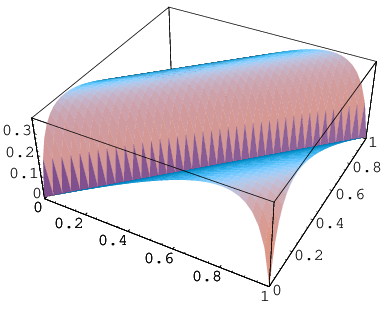
where with . This specification of the volatility function is inspired by Example 1 of Xu and Phillips (2008) (see also Cavaliere (2004)). In Figure 1, we take , and , so that only the break dates and vary freely. In figure 2 only the break dates vary with in general, and , . In Figure 1 and 2 we plot in the left graphics the second component on the diagonal of and in the right graphics the ratio of .
From the left graphic of Figure 1 it turns out that could be far from zero for larger values of and when the breaking point is located early in the sample. From the right graphic of Figure 1 we can see that the ratio of can be far from 1, however the relation between this ratio and the variations of , is not clear. From the left graphic of Figure 2, it appears that can be far from zero. According to the right graphic of Figure 2, the relative difference between and is significantly larger when the breaking points and are located at the end of the sample. This example shows that the standard results for the analysis of the autocovariances can be quite misleading when the unconditional homoscedasticity assumption on the innovations process does not hold.
We also consider the vector of residual autocorrelations: for a given integer , define
with , , and
with , . Since has identity variance matrix, we can also define
Proposition 2
If model (1.1) is correct and Assumption A1 holds true, we have
| (3.13) |
where
where . Moreover,
| (3.14) |
where stands for any of or .
4 Modified portmanteau tests based on OLS estimation
Corrected portmanteau tests based on the OLS residual autocorrelations are proposed below. We use the standard Box-Pierce statistic, Box and Pierce (1970), introduced in the VAR framework by Chitturi (1974)
| (4.1) | |||||
We also consider the Ljung-Box statistic (Ljung and Box (1978)) introduced in the VAR framework by Hosking (1980)
The following result, a direct consequence of Proposition 1 equation (3.13), provides the asymptotic distribution of and .
Theorem 4.1
If model (1.1) is correct and Assumption A1 holds true, the statistics and converge in law to
| (4.2) |
as , where is the vector of the eigenvalues of the matrix
and the ’s are independent variables.
When the error process is homoscedastic i.i.d. and is large, it is well known that the asymptotic distribution of the statistics and under the null hypothesis can be approximated by a chi-square law with degrees of freedom, see Box and Pierce (1970). In our framework, even for large , the limit distribution in (4.2) can be very different from a chi-square law. The following example illustrate this point.
Example 4.1
Consider the bivariate process in Example 3.1. Then
with
If we suppose that is constant and , we obtain , so that the asymptotic distribution of and is with and . However it is easy to see that the non zero diagonal elements in can be far from one if the error process is heteroscedastic. From the Jensen inequality the components and are greater or equal than one. For illustration, in the right graphics of Figures 1 and 2 we present the second diagonal element of when the volatility function is like in (3.11)-(3.12).
Estimates of the weights which appear in (4.2) can be obtained as follows. First, let us recall the following results proved by Patilea and Raïssi (2010):
| (4.3) |
| (4.4) |
| (4.5) |
and
| (4.6) |
A consistent estimator of and given in (3.1) and (3.2) is easily obtained by replacing with their OLS estimators in and using (4.3) and (4.4). Thus from this and the equations (4.3) to (4.6), one can easily define a consistent estimator of . Denote the estimated eigenvalues of by .
We are now ready to introduce the OLS residuals-based corrected versions of the Box-Pierce (resp. Ljung-Box) portmanteau tests for testing the order of the VAR model (1.1). With at hand a vector , at the asymptotic level , the Box-Pierce (resp. Ljung-Box) procedure consists in rejecting the null hypothesis (1.2) of uncorrelated innovations when
(resp. The -values can be evaluated using the Imhof algorithm (Imhof, 1961) or the saddle point method, see e.g. Kuonen (1999).
Let us end this section with some remarks on the particular case (that includes the univariate AR(p) models with time-varying variance). In this case
| (4.7) |
and clearly, . If in addition , by Proposition 1 we have and hence .
5 Adaptive portmanteau tests
An alternative way to build portmanteau tests for VAR(p) models with time-varying variance we consider herein is to use approximations of the innovation . A nonparametric estimate of the volatility function is needed for building such approximations. For this purpose we generalize the approach of Xu and Phillips (2008) to the multivariate case, see also Patilea and Raïssi (2010). Let us denote by the Hadamard (entrywise) product of two matrices of same dimension and . Define the symmetric matrix
where, as before the ’s are the OLS residuals and the element, , of the matrix of weights is given by
with the bandwidth and
The kernel function is bounded nonnegative and such that . For all the bandwidth belongs to a range with some constants and at a suitable rate that will be specified below.
When using the same bandwidth for all the cells of , since , are almost sure linear independent each other, is almost sure positive definite provided is sufficiently large. When using several bandwidths a regularization of could be necessary in order to ensure positive definiteness. Let us consider
where , , is a sequence of real numbers decreasing to zero at a suitable rate that will be specified below. Our simulation experiments indicate that in applications with moderate and large samples could be even set equal to 0.
In practice the bandwidths can be chosen by minimization of a cross-validation criterion like
with respect to all , , where is some norm for a square matrix, for instance the Frobenius norm that is the square root of the sum of the squares of matrix elements. Like in Patilea and Raïssi (2010), the theoretical results below are obtained uniformly with respect to the bandwidths and this provides a justification for the common cross-validation bandwidth selection approach in the framework we consider.
Let us now introduce the following adaptive least squares (ALS) estimator
with
The ALS residuals, proxies of the infeasible GLS residuals, are defined as and the adaptive autocovariances and autocorrelations
where , , and is the nonparametric estimator obtained from and the identification condition on (see Assumption A1(i)), that is .
Let . Following the notation of the previous section, for a given integer , define the residual autocorrelations
The main result of this section shows that and are asymptotic equivalent to and . This will allow us to define new portmanteau statistics based on the ALS residuals. For this purpose, we need the following assumptions.
Assumption A1’: Suppose that all the conditions in Assumption A1(i) hold true. In addition:
(i) where for any symmetric matrix the real value denotes its smallest eigenvalue.
(ii) for all .
Assumption A2: (i) The kernel is a bounded density function defined on the real line such that is nondecreasing on and decreasing on and . The function is differentiable except a finite number of points and the derivative is an integrable function. Moreover, the Fourier Transform of satisfies .
(ii) The bandwidths , , are taken in the range with and as , for some .
(iii) The sequence is such that
Below, we say that a sequence of random matrices , is uniformly with respect to (w.r.t.) as if . The following proposition gives the asymptotic behavior of variances, autocovariances and autocorrelations estimators based on the ALS estimator of and the nonparametric estimate of the time-varying variance structure . The results are uniformly w.r.t the bandwidths.
Proposition 3
If model (1.1) is correct and Assumptions A1’ and A2 hold, uniformly w.r.t.
| (5.1) |
| (5.2) |
Moreover, given any ,
| (5.3) |
where (resp. ) stands for any of and (resp. and ).
This asymptotic equivalence result allows us to propose portmanteau test statistics adapted to the case of time-varying variance. Consider the Box-Pierce type statistic
and
Consider also the Ljung-Box type statistics
and
The following theorem is a direct consequence of (3.7) and Proposition 3 and hence the proof is omitted.
Theorem 5.1
Under the assumptions of Proposition 3, the statistics , and , converge in distribution to
| (5.4) |
as , where is the vector of the eigenvalues of and the ’s are independent variables.
To compute the critical values of the adaptive portmanteau tests, we first obtain a consistent estimator of given in (3.3) by replacing by their ALS estimators in and using (5.1). Next we consider the estimate of given in (5.2). Plugging these estimates into the formula (3.8), we obtain a consistent estimator of with eigenvalues that consistently estimate .
There are several important particular cases that could be mentioned. In the case of a VAR(0) model (i.e., the process is observed), (see Proposition 1) and hence the asymptotic distribution of the four test statistics in Theorem 5.1 would be , that means independent of the variance structure given by . In the general case where the autoregressive coefficients , have to be estimated, the matrix being positive semi-definite, the eigenvalues are smaller or equal to 1. Since, in some sense, the unconditional heteroscedasticity is removed in the ALS residuals, one could expect that the asymptotic approximation is reasonably accurate for the ALS tests. Example 3.1 indicates that this is may not the case, the asymptotic distribution we obtain for the ALS portmanteau statistics can be very different from the approximation when the errors are heteroscedastic. Finally note that Patilea and Raïssi (2010) pointed out that using the adaptive estimators of autoregressive parameters instead of the OLS estimators lead to a gain of efficiency, so that it is advisable to compute the kernel smoothing estimator of the variance function at the estimation stage. Therefore since the kernel estimator of the variance is available for the validation stage, the ALS tests are not more complicated than the OLS tests to implement.
Let us also point out that the eigenvalues will not depend on the variance structure when (in particular in the univariate case), whatever the value of is. Moreover, using the arguments of Box and Pierce (1970), see also Brockwell and Davis (1991, pp. 310–311), one can easily show that for large values of , the law of is accurately approximated by a distribution. However, in the general the multivariate setup the asymptotic distribution in (5.4) depend on the variance function .
6 Modified portmanteau statistics with standard chi-square asymptotic distributions
In the previous sections we considered portmanteau tests for which the asymptotic critical values are given by weighted sums of chi-squares in the general VAR(p) case. Using a suitable change of our quadratic forms one can propose alternative portmanteau test statistics with chi-squared asymptotic distributions under the null hypothesis. This type of modification was already proposed in the recent time series literature but in different contexts.
First note that as remarked above when testing that the observed process is uncorrelated () and using the standard portmanteau statistic (4.1) we obtain a non standard asymptotic distribution. Then following the approach of Lobato, Nankervis and Savin (2002) we consider the modified portmanteau test statistic
where with defined in equation (4.3). The invertibility of is guaranteed asymptotically by our assumptions. In view of Proposition 1 it is clear that under the null hypothesis of uncorrelated observed process, the asymptotic distribution of the statistic is . Recall that this kind of statistic correction is not necessary to obtain a standard asymptotic distribution for the adaptive portmanteau tests when the non correlation of the observed process is tested.
This approach can be generalized to the case of VAR() models with possibly using the approach of Katayama (2008) for building tests with standard asymptotic distributions. In this part we take . Let us introduce
so that and . From the proof of Proposition 1 (equation (12.18)), it is easy to see that
where is asymptotically normal of mean 0 and variance . Deduce that
where . Now, notice that
From this and the fact that is a projector, deduce that the matrix is idempotent, where
Moreover, since is of full column rank , it is easy to see that the rank of is . A classical result in multivariate data analysis implies
| (6.1) |
Similarly we obtain
| (6.2) |
and we deduce
| (6.3) |
The matrices and could be estimated as suggested in Section 4, see comments after equation (4.6), and hence a modified portmanteau test statistic based on the OLS estimates and having standard chi-square critical values could be derived from equation (6.1). On the other hand, using a nonparametric estimate of one could easily estimate , see Proposition 3 and the comments after Theorem 5.1. Moreover, Proposition 3 allows us to replace with and thus to introduce an adaptive portmanteau test with a modified statistic and standard chi-square critical values based on equation (6.3). Clearly one can consider similar modification for Ljung-Box type statistics.
The chi-square critical values are certainly more convenient for portmanteau tests. Moreover, in section 7 we provide evidence that the test based on the statistic (6.1) could be more powerful, in the Bahadur slope sense, than the OLS estimates based test based on the statistic investigated in Theorem 1.1. However, it is not necessarily true that the modified procedures presented in this section are preferable in applications. Indeed, the empirical evidence presented in Section 9 shows that test statistics like in (6.1) and (6.3) are unstable and induce bad levels even with series of few hundred observations.
7 Testing for autocorrelation in heteroscedastic series: some theoretical power comparisons
In this part we carry out some theoretical power comparisons for the tests we considered above in the important case where the non correlation of the observed process is tested. The case will be considered elsewhere. On one hand we compare the classical Box-Pierce portmanteau test and modified quadratic forms of OLS residual autocorrelations based test introduced in section 6. On the other hand we compare ALS and OLS residual autocorrelations based portmanteau tests. For this purpose we use the Bahadur slope approach that we briefly recall here. Let denote a test statistic and, for any , define where stands for the limit distribution of under the null hypothesis. Following Bahadur (1960) (see also van der Vaart 1998, chapter 14), consider the (asymptotic) slope under a fixed alternative such that the limit exists in probability. The asymptotic relative efficiency of the test based on with respect to a competing test based on a test statistic is then defined as the ratio . A relative efficiency suggests that the test given by is better suited to detect because the associated values wanes faster or equally faster compared to the values of the test based on .
For the sake of simplicity we restrict our attention to the BP statistics and consider the case where one tests the non correlation of the observed process, while the underlying true process is the autoregressive process of order 1
| (7.1) |
where for all and . We keep the notation and we introduce . Under the alternative hypothesis (7.1) we have the relationship
| (7.2) |
Using similar arguments to that of the proofs of Lemmas 12.1 to 12.3 in the Appendix, deduce that
| (7.3) |
and
| (7.4) |
Using basic properties of the vec() operator and the Kronecker product we obtain
and
with and .
Proposition 4
(i) If Assumption A1 holds true and the observations follow the model (7.1), the asymptotic relative efficiency of the portmanteau test based on with respect to the portmanteau tests based on is larger or equal to 1.
(ii) Suppose that where is some positive scalar function. Suppose that Assumptions A1’ and A2 holds true and the observations follow the model (7.1). Then asymptotic relative efficiencies of the portmanteau test based on with respect to the portmanteau tests based on or are larger or equal to 1.
In the first part of Proposition 4 the result is obtained without additional restriction on while in the second part we impose which is for instance true in the univariate case (). In the general multivariate case the portmanteau test based on ALS residual autocorrelations does not necessarily outperforms, in the sense of the Bahadur slope, the tests based on the OLS residual autocorrelations considered above.
8 Extending the scope: testing the order of a heteroscedastic co-integration model
Consider the case of a unit root multivariate process with time-varying volatility, see for instance Cavaliere, Rahbek and Taylor (2010) or Boswijk (2010). With the model (1.1) can be rewritten in its error correction form
| (8.1) | |||
The matrices are functions of the ’s, and such that the assumptions of the Granger representation theorem hold (see for instance Assumption 1 of Cavaliere, Rahbek and Taylor (2010)), where the -dimensional matrices and are identified in some appropriate way (see e.g. Johansen 1995, p. 72, for the identification problem). If the sum in (8.1) vanishes. In this section we follow Cavaliere, Rahbek and Taylor (2010) and we slightly strengthen A1 assuming that is iid. Then it follows from their Lemma 1 that have a random walk behavior and also that is stable. By analogy with the homoscedastic case, the number of independent linear stable combinations in is the cointegrating rank (see section 2.3 of Cavaliere, Rahbek and Taylor 2010, for a detailed discussion on the concept of cointegration in our framework). If the process is not cointegrated and the procedures described in the previous sections apply directly to the process . Many contributions in the literature that considered the standard homoscedastic framework pointed out that the choice of the lag length is important for the contegrating rank analysis, see e.g. Boswijk and Franses (1992, section 4). It seems reasonable to imagine that a similar remark remains true with a time-varying variance.
To describe the estimation procedure of (8.1), let us define for any -matrix and rewrite model (8.1) under the form
where . The estimator of the long run relationships can be obtained using the reduced rank regression method introduced by Anderson (1951). Cavaliere et al (2010) showed that in our framework
| (8.2) |
Now, let us define
where
and similarly to (2.2) let us introduce
with
where the volatility is assumed known. Next, for any fixed , let us define the estimated residuals
and the corresponding estimated autocovariance matrices
From (8.2) we obviously have
Defining
it is also obvious that
It is clear now that one can treat as known and, following the lines of the previous sections, one can use and the ALS version of to build portmanteau tests for checking the order of the model (8.1).
9 Monte Carlo experiments
In the sequel and will denote the Ljung-Box type portmanteau tests based on the adaptive approach with non standard distributions (4.2) and (5.4). For the sake of brevity, only the results obtained with the test statistic will be reported. Moreover, since we found similar results for the and tests, we only report on tests. The tests based on modified statistics which are built using the results in Section 6 are denoted by and . If we assume that the volatility function is known, one can also build portmanteau tests using the result in (3.14) in a similar way to the adaptive portmanteau tests. These infeasible tests denoted by and will serve as a benchmark for comparison with the ALS tests and . It is clear that the asymptotic critical values of the ALS tests are the same as the critical values of the GLS tests. In this section we investigate by simulations the finite sample properties of the ALS and GLS portmanteau tests and we compare them with the OLS estimation-based tests. In the next section we study the model adequacy of two real data sets: the US energy and transportation price indexes for all urban consumers on one hand and the US balances on merchandise trade and on services on the other hand.
9.1 Empirical size
Our Monte Carlo experiments are based on the following Data Generating Process (DGP) specification
| (9.1) |
where in the empirical size part of the study and in the empirical power part. The autoregressive parameters are such that the stability condition hold and are inspired from the ALS estimation obtained for the U.S. balance on services and merchandise trade data (see Table 5 below). In the case of smooth variance structure we consider
| (9.2) |
where we take and . In order to investigate the properties of the tests when a volatility break is present we also consider the following specification
| (9.3) |
with and . In this case we have a common volatility break at the date . In all experiments we fix . These volatility specifications are inspired by the real data studies we consider in the next section. For instance to fix the component of the specification (9.2) we noticed that the last estimated variances with the balance services and merchandise trade data are all greater than 200. In the energy-transport price indexes data some of the last estimated variances of the first component are even greater than 300. The amplitudes of the functions and in the volatility specification with an abrupt break defined in (9.3) were calibrated close to the means of the first estimated volatilities and of the last volatilities for the balance services and merchandise trade data. To assess the finite sample properties of the tests under comparison when the errors are stationary, we also considered standard i.i.d. Gaussian error processes. For each experiment independent trajectories are simulated using DGP (9.1). Samples of length , and are simulated.
We first study the empirical size of the tests taking , and adjusting a VAR(1) model to the simulated processes. The portmanteau tests for the non correlation of the error terms are applied using and at the asymptotic nominal level 5%. The results are given in Tables 1, 2 and 3. Since replications are performed and assuming that the finite sample size of the tests is , the relative rejection frequencies should be between the significant limits 3.65% and 6.35% with probability 0.95. Then the relative rejection frequencies are displayed in bold type when they are outside these significant limits. Note that the distributions (4.2) and (5.4) are given for fixed , while the approximation (see discussion after Theorem 4.1 above) should be accurate only for large . Therefore we only comment the results for small and moderate samples ( and ) for the standard portmanteau tests with , while the results for large samples () are considered when is taken.
In Table 1 i.i.d. standard Gaussian errors are used, that means . In this simple case the relative rejection frequencies of the tests converge to the asymptotic nominal level. In general we do not remark a major loss of efficiency of the test when compared to the standard test. Therefore one can use the test in case of doubt of the presence of unconditional heteroscedasticity. The same remark can be made for the test when is small. However we note that the is oversized for small samples and when is large. It also appears that the tests based on modified statistics are oversized when is large. This can be explained by the fact that the matrices and are difficult to invert in such situations.
In Table 2 heteroscedastic errors with an abrupt volatility break are considered, while the trending specification (9.2) is used for the volatility in Table 3. In line with the theoretical the relative rejection frequencies of the ALS, GLS and OLS tests converge to the asymptotic nominal level. As expected the standard portmanteau test is not valid. In general it emerges from this part that the and tests have similar results. Then it seems that estimating the volatility entails no major loss of efficiency when building this kind of test. We did not found clear advantage for the when compared to the in the presented experiments. However note that the asymptotic distribution (4.2) of the standard portmanteau statistic seems estimated with less precision than the asymptotic distribution of the ALS portmanteau statistic. For instance we see in Table 4 that for the standard deviations of the ALS weights are lower or equal to the standard deviations of the OLS weights. We found that this difference is more marked for which may lead to problems for the control of the error of first kind for the as already noted in the homoscedastic case (see Table 1 for ). Other simulation results not reported here show that the test can be oversized when is large as in the homoscedastic case with and we noted that the estimation of the weights requires a relatively large number of observations for the OLS approach. A possible explanation is also that while for , which may proceed more instable estimation for in many cases. In addition the energy-transportation price indexes example below show that the estimation of the weights may be problematic in the OLS case. Therefore we recommend to choose small when the samples are small and use large only when the samples are large despite the asymptotic results hold true for fixed when the is considered. We again note that the tests with modified statistics are in general clearly oversized. A possible explanation is that White (1980) type correction matrices are inverted in the modified portmanteau statistics which may lead to oversized tests as pointed out in Vilasuso (2001) in the stationary case. We can conclude that with a data generating process close to our simulation design the test controls reasonably well the error of the first kind in all the situations we considered.
9.2 Empirical power
In the empirical power part of this section, we examine the ability of the different tests to detect underspecified autoregressive order. The power investigation is realized in the Bahadur sense, that is the sample size is increased while the alternative is kept fixed. More precisely we set , and we adjusted a VAR(1) model to the simulated VAR(2) processes with . We simulated independent trajectories using DGP (9.1) with standard Gaussian innovations and heteroscedastic volatility specifications (9.2) and (9.3). The non correlation of the error process is again tested at the asymptotic nominal level 5%, but taking in all the experiments. In Figure 3 we consider the homoscedastic case, errors where an abrupt volatility shift is observed and errors with smoothly varying variance.
When the variance is constant it appears that the tests with non standard distribution have similar power to the standard test when the errors are homoscedastic. Therefore we again note that there is no major loss of efficiency when the tests with modified distribution are used while the variance is constant. The tests with standard distribution may seem more powerful when the samples are small, but this mainly comes from the fact that these tests are oversized. When the errors are heteroscedastic the standard test seems more powerful than the other tests. However the standard test is oversized and in this case and the comparison is again not fair. A similar comment can be made when the tests with modified distribution are compared to the tests with standard distribution. It emerges that the test is more powerful than the . The relation between the powers of and is not clear. Finally we can remark that in the presented experiments the GLS type tests are not necessarily more powerful than the ALS tests.
The results of section 7 are also illustrated. To this aim independent trajectories are simulated using a VAR(1) DGP with . We consider heteroscedastic errors with trending behavior volatility specification:
where we take , and a volatility with an abrupt shift at :
where . The lengths of the simulated series are . The non correlation of the observed process is tested at the asymptotic nominal level 5% taking . From Figure 4 the test may appear more powerful than the test when the samples are small. However this comes from the fact that the test is strongly oversized in small samples. In accordance with the theoretical we see that the test clearly outperform the and as the samples become large.
10 Illustrative examples
For our real data illustrations we use two U.S. economic data sets. First we consider the quarterly U.S. international finance data for the period from January 1, 1970 to October 1, 2009: the balance on services and the balance on merchandise trade in billions of Dollars. The length of the balance data series is . We also consider monthly data on the U.S. consumer price indexes of energy and transportation for all urban consumers for the period from January 1, 1957 to February 1, 2011. The length of the energy-transportation series is . The series are available seasonally adjusted from the website of the research division of the Federal Reserve Bank of Saint Louis.
10.1 VAR modeling of the U.S. balance trade data
In our VAR system the first component corresponds to the balance on merchandise trade and the second corresponds to the balance on services trade. From Figure 5 it seems that the series have a random walk behavior. We applied the approach of unit root testing proposed by Beare (2008) in presence of non constant volatility using the Augmented Dickey-Fuller (ADF) test for each series. The ADF statistic is for the merchandise trade balance data and is for the services balance data. These statistics are greater than the 5% critical value of the ADF test, so that the stability hypothesis have to be rejected for the studied series. Furthermore we also applied the Kolmogorov-Smirnov (KS) type test for homoscedasticity considered by Cavaliere and Taylor (2008, Theorem 3) for each series. The KS statistic is for the merchandise trade balance data and is for the services balance data. These statistics are greater than the 5% critical value , so that the homoscedasticity hypothesis has to be rejected for our series. Therefore we consider the first differences of the series to get stable processes, so that the evolutions of the U.S. balance data are studied in the sequel. From Figure 6 we see that the first differences of the series are stable but have a non constant volatility. We adjusted a VAR(1) model to capture the linear dynamics of the series. The ALS and OLS estimators are given in Table 5. The standard deviations into brackets are computed using the results (2.3) and (2.4). In accordance with Patilea and Raïssi (2010), we find that the ALS estimation method seems better estimate the autoregressive parameters than the OLS estimation method, in the sense that the standard deviations of the ALS estimators are smaller than those of the OLS estimators. The bandwidth we use for the ALS estimation, , is selected by cross-validation in a given range and using 200 grid points (Figure 7).
A quick inspection of Figures 8 and 9 suggests that the OLS residuals have a varying volatility, while the stationarity of the ALS residuals is plausible. Thus it seems that the volatility of the error process is satisfactorily estimated by the adaptive method. Now we examine the possible presence conditional heteroscedasticity in the ALS residuals. From Figure 10 we see that the autocorrelations of the squared ALS residuals components are not significant. In addition we also considered the ARCH-LM test of Engle (1982) with different lags in Table 6 for testing the presence of ARCH effects in the ALS residuals. It appears that the null hypothesis of conditional homoscedasticity cannot be rejected at the level 5%. These diagnostics give some evidence that the conditional homoscedasticity assumption on is plausible in our case. To analyze the changes of the variance of the OLS error terms, we plotted the estimated variances and cross correlation of the components of the error process in Figures 11 and 12. It appears from Figure 11 that the variance of the first component of the residuals does not vary much until the end of the 90’s and then increase. Similarly the volatility of the second component of the residuals does not vary much until the end of the 80’s and then increase. From Figure 12 we also note that the correlation between the components of the innovations seems to be positive until the beginning of the 90’s and then become negative.
Now we turn to the check of the goodness-of-fit of the VAR(1) model adjusted to the first differences of the series. To illustrate the results of Proposition 1 we plotted the ALS residual autocorrelations in Figures 13 and 14, and the OLS residual autocorrelations in Figures 15 and 16, where we denote
The ALS 95% confidence bounds obtained using (3.14) and (5.3) are displayed in Figures 13 and 14. In Figures 15 and 16 the standard 95% confidence bounds obtained using (3.9) and the OLS 95 % confidence bounds obtained using (3.13) are plotted. We can remark that the ALS residual autocorrelations are inside or not much larger than the ALS significance limits. A similar comment can be made for the OLS residual autocorrelations when compared to the OLS significance limits. However we found that the OLS significance limits can be quite different from the standard significance limits. This can be explained by the presence of unconditional volatility in the analyzed series. In particular we note that the is far from the standard confidence bounds. We also apply the different portmanteau tests considered in this paper for testing if the errors are uncorrelated. The test statistics and -values of the tests are displayed in Tables 7 and 8. It appears that the -values of the standard tests are very small. Therefore the standard tests clearly reject the null hypothesis. We also remark that the -values of the modified tests based on the OLS estimation and of the adaptive tests are far from zero. Thus in view of the tests introduced in this paper the null hypothesis is not rejected. These contradictory results can be explained by the fact that we found that the distribution in (4.2) is very different from the standard distribution. For instance we obtained for in our case. Our findings may be viewed as a consequence of the presence of unconditional heteroscedasticity in the data. Since the theoretical basis of the standard tests do not include the case of stable processes with non constant volatility, we can suspect that the results of the standard tests are not reliable. Therefore we can draw the conclusion that the practitioner is likely to select a too large autoregressive order in our case when using the standard tools for checking the adequacy of the VAR model. From Table 8 we see that the OLS and ALS statistics are quite different. We also noted that the weights (not reported here) of the sums in (4.2) and in (5.4) are quite different for our example.
10.2 VAR modeling of the U.S. energy-transportation data
In this example the first component of the VAR system corresponds to the transportation price index and the second corresponds to the energy price index. We first briefly describe some features of the energy-transportation price indexes. In Figure 17 we again see that the studied series seems to have a random walk behavior and then we again consider the first differences of the series. The KS type statistic is for the energy price index and is for the transportation price index, so that the homoscedasticity hypothesis has to be rejected for these series. From Figure 18 we see that the first differences of the series are stable but have a non constant volatility. We adjusted a VAR(4) model to capture the linear dynamics of the series. The results in Table 9 indicate that the ALS approach is more precise than the OLS approach for the estimation of the autoregressive parameters. The bandwidth obtained by the cross-validation for the ALS estimation is (Figure 19). From Figure 21 we see that the OLS residuals seem to have a varying volatility. The stationarity of the ALS residuals is plausible (Figure 20) and ARCH-LM tests (not reported here) show that the conditional homoscedasticity of the ALS residuals cannot be rejected. From Figure 22 we see that the shape of the variance structure of the components of the OLS residuals are similar. More precisely it can be noted that the variance of the components of the OLS residuals is relatively low and seems constant until the beginning of the 80’s. The OLS residual variance seems to switch to an other regime where the variance is increased but constant from the beginning of the 80’s to the end of the 90’s. The volatility of the OLS residual variance seems to increase from the end of the 90’s. From Figure 12 we also note that the components of the OLS residuals seem highly correlated.
Now we check the adequacy of the VAR(4) model. The ALS and OLS residual autocorrelations are given in Figures 24, 25 and 26, 27. The OLS residual autocorrelations with the standard bounds are given in Figures 28 and 29. From Figures 24 and 25 it can be noted that the ALS residual autocorrelations are inside or not much larger than the ALS significance limits. The OLS confidence bounds seems not reliable since we remark that some confidence bounds (corresponding to the ’s) are unexpectedly much larger than the OLS residual autocorrelations. From Figures 28 and 29 it can also be noted that some of the OLS residual autocorrelations are far from the standard confidence bounds. However considering the standard confidence bounds in presence of non constant variance can be misleading in view of our theoretical findings. In addition we also remark that some standard confidence bounds (corresponding to the , and , ) are unexpectedly far from the residual autocorrelations. The non correlation of the residuals is tested using the different portmanteau tests considered in this paper. The test statistics and -values of the tests are displayed in Tables 10 and 11. The standard tests again lead to select complicated models since the adequacy of the VAR(4) model is rejected. We also remark that the -values of the OLS tests are very large. In fact we found that the OLS tests do not reject the hypothesis of the adequacy of a VAR(1) model for the studied series. From Table 12 we see that some of the estimated weights for the asymptotic distribution of the standard statistic take very large values. It appears that the OLS method seems not able to estimate correctly the asymptotic distribution of the standard statistics and may be suspected to have a low power in this example. Then the OLS portmanteau test seem not reliable in this example on the contrary to the ALS portmanteau test. Indeed it can be noted that the asymptotic distribution seems well estimated. Finally note that we found that the estimators of the and are not invertible, so that the and are not feasible in this example. In view of the different outputs we presented, it seems that the test is the only test which give reliable conclusions in this example. This may be explained by the fact that the variance strongly change in this second example when compared to the first example and hence make the tests based on inverted matrices or the tests which do not exploit the variance structure difficult to implement.
11 Conclusion
In this paper the problem of specification of the linear autoregressive dynamics of multivariate series with deterministic but non constant volatility is studied. Considering such situations is important since it is well known that economic or financial series commonly exhibit non stationary volatility. The unreliability of the standard portmanteau tests for testing the adequacy of the autoregressive order of VAR processes is highlighted through theoretical results and empirical illustrations. From the statistical methodology point of view, the main contribution of the paper is two-fold. In the setup of a stable VAR with time-varying variance, (a) we show how to compute corrected critical values for the standard portmanteau statistics implemented in all specialized software; and (b) we propose new portmanteau statistics based on the model residuals filtered for the non constant variance. Moreover, we provide some theoretical and empirical power comparisons of the two approaches and we show that they are well-suited for replacing the usual test procedures even when the volatility is constant. The new portmanteau statistics require the estimation of the time-varying variance that is done by classical kernel smoothing of the outer product of the OLS residuals vectors. Then another contribution of the paper is represented by the fact that our asymptotic results are derived uniformly in the bandwidth used in the kernel. This makes the theory compatible with the practice where people usually use the data to determine the bandwidth. Our theoretical and empirical investigation could be extended to other setups, like for instance the co-integrated systems. We briefly mention this extension but a deeper investigation is left for future work.
12 Appendix A: Proofs
For the sake of a simpler presentation, hereafter we stick to our identification condition for and hence we replace everywhere by . Recall that
(see pages 2 and 3). Let us introduce
and
for a given . To prove Propositions 1 and 2 we need several preliminary results that are gathered in Lemmas 12.1 to 12.3 below.
Lemma 12.1
Proof of Lemma 12.1 Statement 12.1 is a direct consequence of Lemma 7.2 in Patilea and Raïssi (2010). For the proof of (12.2) we write22 2 Here we make a common abuse of notation because in Assumption A1 the matrix-valued function is not defined for negative values. To remedy this problem it suffices to extend the function to the left of the origin, for instance by setting equal to the identity matrix if .
Therefore
Similarly we have
| (12.4) |
so that using (12.1) we obtain the result (12.2). The proof of (12.3) is similar.
Let us define and . The following lemma is similar to Lemma 7.3 of Patilea and Raïssi (2010), and hence the proof is omitted.
Lemma 12.2
Under A1 we have
| (12.5) |
| (12.6) |
for , and
| (12.7) |
| (12.8) |
In addition we have
| (12.9) |
| (12.10) |
Lemma 12.3
Under A1 we have
| (12.11) |
| (12.12) |
In addition we also have
| (12.13) |
| (12.14) |
where
and
Proof of Lemma 12.3 Statements (12.11) and (12.12) lemma are direct consequences of Lemma 7.4 of Patilea and Raïssi (2010). We only give the proof of (12.14) and (12.13). To prove (12.14), using the well known identity for matrices of appropriate dimensions, we obtain
From (12.10) we write
Now let us denote the discontinuous points of the functions by where is a finite number independent of . We write
Then from (12.3) we obtain
where
and . Noting that are martingale differences, we obtain the result (12.14) using the Lindeberg central limit theorem. Using relations (12.2) and (12.9), the proof of (12.13) is similar. Finally, the equivalent compact expressions of and can be easily derived using elementary properties of the Kronecker product.
Proof of Proposition 1 First we establish the result (3.5). Let us define
Let us first show the asymptotic normality of . Note that
with . From (12.12) we write
with
Then we can obtain from (12.13)
| (12.16) |
with defined in Lemma 12.3. Now, define with . Considering and as values of the same function at the points and , by the Mean Value Theorem
with between and .33 3 The value between and may be different for different components of and . Using and since , it follows from (12.5) and (12.7) that
| (12.17) | |||||
From (12.2) and using arguments like in the proof of (12.14), it is easy to see that
Finally from (12.17) we have
| (12.18) |
so that it follows from (12.16) that is asymptotically normal with covariance matrix
| (12.19) |
The proof of (3.7) is very similar, here we only present a sketch. Let us define
Using (12.11) and (12.14) it can be shown that
| (12.20) |
with defined in Lemma 12.3 and
From (12.6), (12.8) and since we write
By (12.20), is asymptotically normal with covariance matrix The particular case where the order of the VAR model is is an easy consequence of the arguments above in this proof.
Proof of Proposition 2 For the proof of (3.13), we write
It is clear from (12.4) that
where is the th diagonal element of . Following similar arguments used in Phillips and Xu (2005 p 303) for the proof of Lemma 1 (iii), we write
Let us define and . We have using again the Mean Value Theorem
with is between and .44 4 The value may be different for different components of and . Therefore using and from the consistency of , we write
and
so that the result follows from the Slutsky lemma. We obtain the expression (3.13) noting that
The proof of (3.14) is similar to that of (3.13) and hence is omitted.
Proof of Proposition 3 In the following, , , … denote constants with possibly different values from line to line. To simplify notation, let denote the vector of bandwidths , . Below we will simply write uniformly w.r.t. instead of uniformly w.r.t. , , and instead of . Here the norm is the Frobenius norm which in particular is a sub-multiplicative norm, that is , and for a positive definite matrix , with a constant depending only on the dimension of . Moreover, .
To obtain the asymptotic equivalences in equation (5.3) it suffices to notice that for all , , and to prove
| (12.21) |
and
| (12.22) |
for any fixed . Let us write
where with
By Lemma 12.4-(a,b) and given that and , we obtain that
| (12.23) |
From this and the moment conditions on induced by Assumption A1, deduce that (12.21) holds true. On the other hand,
The terms and could be handled in a similar manner, hence we will only analyze . Let us write
By (12.23) and the moment conditions on the innovation process , and the rate of convergence of and 12.4-(b), it is clear that . Next let us write
where, like in Patilea and Raïssi (2010),
From classical matrix norm inequalities (see for instance Horn and Johnson, 1994), we have that for any positive definite matrices and , for or ,
| (12.24) |
where is a constant that depends only on (by definition ). Applying this inequality twice we deduce
Take the norm of , use the inequality in the last display, Lemma 12.4-(a) below, the moment conditions on the innovation process and the condition to deduce that . Next, using similar matrix norm inequalities, Lemma 12.4-(a) and the Cauchy-Schwarz inequality,
where for the equality we used Lemma 7.6-(i) in Patilea and Raïssi (2010). Deduce that . The uniform rate of convergence for is obtained after replacing by a Taylor expansion of the power function for positive definite matrix, a key and apparently new ingredient we provide in section 12.1 below. The reminder term of the Taylor expansion could be controlled taking expectation, using Cauchy-Schwarz inequality and Lemma 12.4-(d). The term under the integral that represents the first order term of this Taylor expansion could be treated similarly to the term in the proof of the Proposition 4.1 of Patilea and Raïssi (2010). That means we use the CLT for m.d. sequences indexed by classes of functions, see Bae, Jun and Levental (2010), see also Bae and Choi (1999). Here the uniformity to be considered is also with respect to the integration variable , but this can be handled with very little additional effort, like in Patilea and Raïssi (2010). The details are omitted. Finally, to derive the uniform order , let us write it as
The term is centered and the variance of each element of this matrix decreases to zero at the rate (use Lemma 12.4-(d) and Assumption A1’ to derive the rate of the variance). Deduce that . Next consider the stochastic processes corresponding to the elements of and indexed by where . For each such process apply Theorem 1 of Bae, Jun and Levental (2010) to deduce that . Finally, deduce that
To handle the term , let us write
The term could be easily handled taking the norm, using the bound on and Lemma 12.4-(b) below. For , we could decompose in four term exactly as we did for and apply the same techniques. The details are omitted and are available from the authors upon request.
Lemma 12.4
Let denote the Frobenius norm. Under the Assumptions of Proposition 3 we have:
(a) As , for or , we have
(b) As ,
(c) As ,
(d) As ,
| (12.25) |
The proof of Lemma 12.4 is a direct consequence of Lemmas 7.5 and 7.6 of Patilea and Raïssi (2010) and Lemma A of Xu and Phillips (2008) applied elementwise, and hence will be omitted.
Proof of Proposition 4 The notation in this proof are those of section 7. First let us notice that for large values of , provided the asymptotic law of a test statistic under the null hypothesis is with some . In the case where a test statistic has the asymptotic distribution of defined in equation (4.2),
and
with and independent variables. Thus to prove (i) it suffices to show that
| (12.26) |
Herein, for any and symmetric matrices, means that is positive semidefinite. Now, in the last display, multiply both sides of the order relationship on the left and on the right by and deduce that it suffices to prove
To obtain (12.26) it remains to notice that and that , are the eigenvalues of .
In (ii) we suppose and in this case it suffices to notice that
where for the order relationship we use Cauchy-Schwarz inequality, while
12.1 A Taylor expansion of the matrix function
Recall that the differential of a function that maps a matrix into a matrix is defined by the equation
where is a vector function such that . In other words, the (first-order) differential of at in the matrix obtained by unstacking the differential of at . See also Schott (2005), section 9.3. Basic properties of vector differentials implies
Now, recall that for any positive definite matrix, the Lyapunov equation has a unique solution that can be represented as
See Horn and Johnson (1991), section 6.5. All these facts brings us to the following technical result.
Lemma 12.5
Let and be two positive definite matrices such that for some constant and and , where is the smallest eigenvalue of the symmetric matrix . Moreover, suppose that for some small constant . Then
where is a symmetric matrix with and is a constant depending only on , .
Proof of Lemma 12.5 Let be some arbitrary matrix. By Taylor expansion, for sufficiently small values of and for some matrices ,
| (12.27) |
with and a constant depending on and the norm of . This kind of representation could be derived from a Taylor formula for the vector function defined by the equation considered in a neighborhood of the for a positive definite matrix . See, for instance, Schott (2005), section 9.6. On the other hand, recall that for a square matrix with , where is the reminder of the expansion with . Thus for sufficiently small values of we can write
| (12.28) | |||||
Taking the square on both sides of the first equality in (12.27) and identifying the coefficients of the power of in equation (12.28) deduce that is the solution of the Lyapunov equation
Finally, the result follows by taking and .
References
-
Ahn, S.K. (1988) Distribution for residual autocovariances in multivariate autoregressive models with structured parameterization. Biometrika 75, 590-593.
-
Anderson, T.W. (1951) Estimating linear restrictions on regression coefficients for multivariate normal distributions. Annals of Mathematical Statistics 22, 327-351.
-
Bae, J., and Choi, M.J. (1999) The uniform CLT for martingale difference of function-indexed process under uniform integrable entropy. Communications Korean Mathematical Society 14, 581-595.
-
Bae, J., Jun, D., and Levental, S. (2010) The uniform CLT for martingale differences arrays under the uniformly integrable entropy. Bulletin of the Korean Mathematical Society 47, 39-51.
-
Baek, E., and Brock, W. (1992) A general test for nonlinear Granger causality: bivariate model. Working paper, University of Wisconsin-Madison.
-
Bahadur, R.R. (1960) Stochastic comparison of tests. Annals of Mathematical Statistics 31, 276-295.
-
Beare B.K. (2008) Unit root testing with unstable volatility. Working paper, Nuffield College, University of Oxford.
-
Boswijk, H.P. (2010) Nuisance parameter free inference on cointegration parameters in the presence of a variance shift. Economics Letters 107, 190-193.
-
Boswijk, H.P., and Franses, H.F. (1992) Dynamic specification and coitengration. Oxford Bulletin of Economics and Statistics 54, 369-381.
-
Boubacar Mainassara, Y. (2010) Multivariate portmanteau test for structural VARMA models with uncorrelated but non-independent error terms. Working paper. EQUIPPE Université Lille 3.
-
Box, G.E.P., and Pierce, D.A. (1970) Distribution of residual autocorrelations in autoregressive-integrated moving average time series models. Journal of the American Statistical Association 65, 1509-1526.
-
Brockwell, P.J., and Davis, R.A. (1991) Time Series: Theory and methods. Springer, New York.
-
Brüggemann R., Lütkepohl H., and Saikkonen P. (2006) Residual autocorrelation testing for vector error correction models. Journal of Econometrics 134, 579-604.
-
Cavaliere, G. (2004) Unit root tests under time-varying variance shifts. Econometric Reviews 23, 259-292.
-
Cavaliere, G., Rahbek, A. and Taylor, A.M.R. (2010) Testing for co-integration in vector autoregressions with non-stationary volatility. Journal of Econometrics 158, 7-24.
-
Cavaliere, G., and Taylor, A.M.R. (2007) Testing for unit roots in time series models with non-stationary volatility. Journal of Econometrics 140, 919-947.
-
Cavaliere, G., and Taylor, A.M.R. (2008) Time-transformed unit root tests for models with non-stationary volatility. Journal of Time Series Analysis 29, 300-330.
-
Chitturi, R. V. (1974) Distribution of residual autocorrelations in multiple autoregressive schemes. Journal of the American Statistical Association 69, 928-934.
-
Duchesne, P. (2005) Testing for serial correlation of unknown form in cointegrated time series models. Annals of the Institute of Statistical Mathematics 57, 575-595.
-
Edgerton, D., and Shukur, G. (1999) Testing autocorrelation in a system perspective. Econometric Reviews 18, 343-386.
-
Engle, R.F. (1982) Autoregressive conditional heteroscedasticity with estimates of the variance of UK inflation. Econometrica 50, 987-1008.
-
Francq, C., and Raïssi, H. (2007) Multivariate portmanteau test for autoregressive models with uncorrelated but nonindependent errors. Journal of Time Series Analysis 28, 454-470.
-
Francq, C., Roy, R., and Zakoïan, J.-M. (2005) Diagnostic checking in ARMA models with uncorrelated errors. Journal of the American Statistical Association 13, 532-544.
-
Horn, R.A., and Johnson, C.R. (1994) Topics in Matrix Analysis. Cambridge University Press, Cambridge.
-
Hosking, J. R. M. (1980) The multivariate portmanteau statistic. Journal of the American Statistical Association 75, 343-386.
-
Imhof, J. P. (1961) Computing the distribution of quadratic forms in normal variables. Biometrika 48, 419-426.
-
Johansen, S. (1995) Likelihood-Based Inference in Cointegrated Vector Autoregressive Models. Oxford University Press, New York.
-
Jones, J.D. (1989) A comparison of lag-length selection techniques in tests of Granger causality between money growth and inflation: evidence for the US, 1959-86. Applied Economics 21, 809-822.
-
Katayama, N. (2008) An improvement of the portmanteau statistic. Journal of Time Series Analysis 29, 359-370.
-
Kim, T.-H., Leybourne, S., and Newbold, P. (2002) Unit root tests with a break in innovation variance. Journal of Econometrics 103, 365-387.
-
Kuonen, D. (1999) Saddlepoint approximations for distributions of quadratic forms in normal variables. Biometrika 86, 929-935.
-
Ljung, G.M. and Box, G.E.P. (1978) On measure of lack of fit in time series models. Biometrika 65, 297-303.
-
Lobato, I., Nankervis, J.C., and Savin, N.E. (2002) Testing for zero autocorrelation in the presence of statistical dependence. Econometric Theory 18, 730-743.
-
Lütkepohl, H. (2005) New Introduction to Multiple Time Series Analysis. Springer, Berlin.
-
Patilea, V., and Raïssi, H. (2010) Adaptive estimation of vector autoregressive models with time-varying variance: application to testing linear causality in mean. Working document IRMAR-INSA; arXiv:1007.1193v2
-
Phillips, P.C.B., and Xu, K.L. (2005) Inference in autoregression under heteroskedasticity. Journal of Time Series Analysis 27, 289-308.
-
Ramey, V.A., and Vine, D.J. (2006) Declining volatility in the U.S. automobile industry. The American Economic Review 96, 1876-1889.
-
Raïssi, H. (2010) Autocorrelation based tests for vector error correction models with uncorrelated but nonindependent errors. Test 19, 304-324.
-
Sensier, M., and van Dijk, D. (2004) Testing for volatility changes in U.S. macroeconomic time series. Review of Economics and Statistics 86, 833-839.
-
Schott, J.R. (2005) Matrix analysis for statistics (2nd ed.).Wiley series in probability and statistics, Wiley, Hoboken, N.J.
-
Stock, J.H., and Watson, M.W. (1989) Interpreting the evidence on money-income causality. Journal of Econometrics 40, 161-181.
-
van der Vaart, A.W. (1998) Asymptotic Statistics. Cambridge University Press, Cambridge.
-
Thornton, D.L. and Batten, D.S. (1985) Lag-length selection and tests of Granger causality between money and income. Journal of Money, Credit, and Banking 17, 164-178.
-
Vilasuso, J. (2001) Causality tests and conditional heteroskedasticity: Monte Carlo evidence. Journal of Econometrics 101, 25-35.
-
Watson, M.W. (1999) Explaining the increased variability in long-term interest rates. Federal Reserve Bank of Richmond Economic Quarterly 85/4, 71-96.
-
White, H. (1980) A heteroskedasticity consistent covariance matrix estimator and a direct test for heteroskedasticity. Econometrica 48, 817-838.
-
Xu, K.L., and Phillips, P.C.B. (2008) Adaptive estimation of autoregressive models with time-varying variances. Journal of Econometrics 142, 265-280.
13 Appendix B: Tables and Figures
| Case | ||||||
|---|---|---|---|---|---|---|
| T | 50 | 100 | 200 | 50 | 100 | 200 |
| 2.6 | 4.6 | 5.5 | 4.4 | 4.1 | 4.6 | |
| 4.2 | 4.9 | 5.2 | 11.5 | 8.1 | 6.9 | |
| 2.2 | 4.1 | 5.1 | 4.1 | 3.7 | 4.4 | |
| 2.0 | 3.9 | 5.1 | 3.7 | 3.8 | 4.3 | |
| 14.2 | 9.0 | 6.5 | 30.9 | 15.4 | 10.5 | |
| 6.3 | 5.9 | 5.6 | 15.8 | 7.4 | 6.8 | |
| 4.6 | 4.7 | 4.8 | 8.6 | 8.1 | 8.1 | |
| Case | ||||||
|---|---|---|---|---|---|---|
| T | 50 | 100 | 200 | 50 | 100 | 200 |
| 27.9 | 35.3 | 40.1 | 35.7 | 63.0 | 76.7 | |
| 4.5 | 3.3 | 4.8 | 5.4 | 6.1 | 6.0 | |
| 3.2 | 3.7 | 5.0 | 3.8 | 3.8 | 3.9 | |
| 2.6 | 4.2 | 5.7 | 3.7 | 4.2 | 4.7 | |
| 28.9 | 13.8 | 9.7 | 30.9 | 21.9 | 15.2 | |
| 18.6 | 8.7 | 7.1 | 35.0 | 15.9 | 9.0 | |
| 6.4 | 5.3 | 6.3 | 12.5 | 10.0 | 9.7 | |
| Case | ||||||
|---|---|---|---|---|---|---|
| T | 50 | 100 | 200 | 50 | 100 | 200 |
| 12.8 | 15.1 | 19.2 | 18.4 | 27.5 | 36.8 | |
| 4.9 | 4.5 | 4.8 | 9.2 | 7.3 | 6.3 | |
| 4.4 | 5.0 | 5.0 | 8.0 | 6.0 | 6.0 | |
| 2.3 | 3.7 | 5.2 | 2.8 | 4.0 | 4.0 | |
| 32.4 | 22.6 | 15.3 | 38.3 | 25.1 | 16.5 | |
| 10.0 | 4.2 | 3.3 | 22.7 | 6.7 | 5.2 | |
| 5.7 | 5.3 | 6.3 | 10.8 | 9.7 | 9.2 | |
| 1 | 2 | 3 | 4 | 5 | |
|---|---|---|---|---|---|
| 6 | 7 | 8 | 9 | 10 | |
| 11 | 12 | 13 | 14 | 15 | |
| 16 | 17 | 18 | 19 | 20 | |
| Parameter | ||||
|---|---|---|---|---|
| ALS estimate | ||||
| OLS estimate |
| lags | 2 | 5 | 10 |
|---|---|---|---|
| 22.26 | 45.05 | 36.44 | |
| 25.32 | 73.32 | 77.18 |
| 5 | 15 | |
|---|---|---|
| 0.00 | 0.01 | |
| 50.80 | 99.94 | |
| 6.36 | 15.95 | |
| 0.00 | 7.87 | |
| 5.61 | 15.50 |
| 5 | 15 | |
|---|---|---|
| 6.84 | 106.34 | |
| 25.73 | 66.83 | |
| 6.84 | 106.34 | |
| 48.73 | 66.83 |
| Parameter | ||||
|---|---|---|---|---|
| ALS estimate | ||||
| OLS estimate | ||||
| Parameter | ||||
| ALS estimate | ||||
| OLS estimate | ||||
| Parameter | ||||
| ALS estimate | ||||
| OLS estimate | ||||
| Parameter | ||||
| ALS estimate | ||||
| OLS estimate |
| 3 | 6 | 12 | |
|---|---|---|---|
| n.a. | 2.08 | 0.00 | |
| 100.00 | 100.00 | 100.00 | |
| 85.44 | 98.72 | 10.07 | |
| n.a. | n.a. | n.a. | |
| n.a. | n.a. | n.a. |
| 3 | 6 | 12 | |
|---|---|---|---|
| 1.87 | 18.06 | 117.51 | |
| 5.03 | 9.50 | 57.69 | |
| n.a. | n.a. | n.a. | |
| n.a. | n.a. | n.a. |
| 1 | 2 | 3 | 4 | 5 | 6 | 7 | 8 | 9 | 10 | 11 | 12 | |
| 0.05 | 0.48 | 1.94 | 2.05 | 2.66 | 2.85 | 4.97 | 6.58 | 10.51 | 16.06 | 64.14 | 312.18 | |
| 0.01 | 0.09 | 0.24 | 0.89 | 1.00 | 1.00 | 1.00 | 1.00 | 1.00 | 1.00 | 1.00 | 1.00 |