Iterative Bias Reduction Multivariate Smoothing in R: The ibr Package
Abstract
In multivariate nonparametric analysis, sparseness of the covariates also called curse of dimensionality, forces one to use large smoothing parameters. This leads to a biased smoother. Instead of focusing on optimally selecting the smoothing parameter, we fix it to some reasonably large value to ensure an over-smoothing of the data. The resulting base smoother has a small variance but a substantial bias. In this paper, we propose an R package named ibr to iteratively correct the initial bias of the (base) estimator by an estimate of the bias obtained by smoothing the residuals. After a brief description of Iterated Bias Reduction smoothers, we examine the base smoothers implemented in the packages: Nadaraya-Watson kernel smoothers and thin plate splines smoothers. Then, we explain the stopping rules available in the package and their implementation. Finally we illustrate the package on two examples: a toy example in and the original Los Angeles ozone dataset.
Keywords:
R,keywords
, and
1 Introduction
Regression is a fundamental data analysis tool for uncovering functional relationships for the conditional expectation from pairs of observations . Classical linear regression is the simplest example of this. More generally, we can let the data help determine the general form of the relationship by using one of the numerous non-parametric regression estimators, such as wavelets based smoothers, kernel smoothers, and splines smoothers (Buja et al., 1989; Cleveland and Devlin, 1988; Eubank, 1988; Fan and Gijbels, 1996; Antoniadis and Oppenheim, 1995; Simonoff, 1996). The latter flexible smoothing methods are implemented as R functions found in numerous contributed packages. For instance the package wavethresh (Nason, 2010) implements a wavelet based smoother, the package lokern (for R and enhanced by Martin Maechler, 2010) provides a kernel smoothers and the function smooth.spline calculates a cubic spline smoother. When the number of dependent variables is greater than 3 or 4, fully non-parametric regression suffers from the curse of dimensionality, even for moderate sample sizes (say being equal to a few hundred). As a result, application of fully non-parametric methods are discouraged in dimensions four and higher. Instead, the statistical literature encourages using constrained non-parametric regression models (additive models (Hastie and Tibshirani, 1990), single and multiple index models and projection pursuit models) to estimate useful approximations of the conditional expectation. The latter methods are provided to the R community in the contributed package mgcv (Wood, 2011) for additive modelling, function ppr for projection pursuit and package mda (Hastie et al., 2011) for MARS.
Originating from the machine learning community, the boosting algorithm is also another tool for non-parametric regression (see Friedman, 2001, and references therein). This fairly recent and very popular method has numerous variations, such as adaboost (the original method), logitboost for classification, and the boosting for regression. The interesting feature is that it provides a framework for combining various weak learners (non-parametric smoothers) into a smoother that is better than any single smoother that it is composed off. Packages for boosting are already available in R: for instance the package mboost (Hothorn et al., 2010) allows for boosting for regression problem as well as logistic boosting for classification. For multivariate regression, the boosting algorithm has been applied to component-wise additive modelling with classical smoother such as smoothing splines (Bühlmann and Hothorn, 2007, see).
Linking the boosting algorithm to an iterative bias correction scheme (see for example Bühlmann and Hothorn (2007) for boosting of smoothing splines and Cornillon et al. (2011) for discussions on boosting of more general smoothers) provides a statistical interpretation of the boosting algorithm. This interpretation was alluded to in Ridgeway (2000)’s discussion of Friedman et al. (2000) paper on the statistical interpretation of boosting. The basic idea of estimating (and correcting for) the bias of a pilot smoother goes back to the concept of twicing introduced by Tukey (1977). The idea of iterating the bias correction was central to adaptive bagging algorithm of Breiman (1999). More details about statistical properties in univariate or multivariate smoother can be found in Bühlmann and Yu (2003) or Cornillon et al. (2011).
This paper focuses on the computational implementation in R (R Development Core Team, 2009) of the iterated bias correction procedure for fully multivariate regression smoothers. We start in Section two by briefly presenting the concept of iterative bias reduction and recalling its connection to boosting. The details of our numerical implementation and a review of available options in our R package ibr are given in Section three. The last section is devoted to examples.
2 Iterative bias reduction smoothers
2.1 Method
Suppose that the pairs are related through the non-parametric regression model
| (1) |
where is an unknown smooth function, and the disturbances are independent mean zero and variance random variables that are independent of all the covariates. It is helpful to rewrite Equation (1) in vector form by setting , and , to get
| (2) |
Linear smoothers estimate the regression function evaluated at the covariates by linear combinations of the responses that can be compactly written as
| (3) |
where is an smoothing matrix with smoothing parameter . By slight abuse of language, we will sometimes refer to the vector of fitted values as the smooth of . Typical smoothers (Hastie et al., 2001, see for instance) include bin smoothers, spline based smoothers (regression splines, smoothing splines, and thin-plate splines), kernel based smoothers (Nadaraya-Watson kernels and local polynomials smoothers), and series based smoothers (Fourier smoothers and wavelet smoothers). In this paper, we focus only on two common types of smoothers: Nadaraya-Watson kernels (where is the bandwidth) and thin-plate splines (where is the penalty parameter). Extensions to other smoothers can easily be achieved by suitably modifying our theoretical results and software.
The linear smoother (3) has bias
and variance
To estimate the bias, observe that the residuals have expected value . This suggests estimating the bias by smoothing the negative residuals
Recall that, in multivariate non-parametric analysis, sparseness of the covariates also called curse of dimensionality, forces one to use large smoothing parameters . This leads to very biased base smoother . Thus the bias correction in multivariate non-parametric analysis arises as a natural tool to correct classical smoother . If is large, not all the bias is usually removed after a the first correction. To remove the remaining bias, iterations of the bias reduction step have to be performed. For instance bias reduction step produces the linear smoother at iteration :
| (4) | |||||
When , the sequence of iterated bias corrected smoothers agrees with the -boosted smoothers without shrinkage. For , the boosting algorithm is applied component-wise to additive regression models (Bühlmann and Yu, 2003, see). This results in a sequence of constrained (additive) approximation of the fully non-parametric regression function .
For thin-plate splines and kernels smoothers (with suitable kernels, such as as a Gaussian density function), each iteration of the bias correction produces a noisier but less biased smoother. In the limit, the sequence of iterative bias corrected smoothers reproduces the raw data (Cornillon et al., 2011). Thus there is a need for good stopping rules for the iterative bias correction algorithm.
To illustrate this behavior, let us use a classical bivariate regression problem: figure 1 graphs Wendelberger’s test function (Wendelberger, 1982):
| (5) | |||||

The sequence of bias corrected thin-plate spline smoothers, starting from a pilot that over-smooths the data, converges to an interpolant of the raw data (see figure 2 (c)). After some suitable number of bias correction steps, the resulting bias corrected smoother will be a good estimate for the true underlying regression function (see figure 2 (b)). The crucial choice of is achieved by the use of classical criterion such as corrected AIC or GCV (see section 2.2).

We note that, provided is large enough, its exact value is not crucial as the choice of will adapt to : if two base smoothers are chosen, one with and another with , the chosen iteration will be greater than as it takes more iterations with a very smooth base smoother to remove the bias.
To make prediction at arbitrary locations of the covariates, we extend linear smoothers to functions of the form
| (6) |
where is a vector of size whose entries are the weights for predicting . The vector reduces to the row of the smoothing matrix when , and is readily computed for many of the smoothers used in practice.
For extended base smoothers of the form (6), we propose to extend the associated iterative bias corrected smoother by observing that
| (7) | |||||
| (8) | |||||
| (9) |
This implies that . Hence we propose to extend the iterative bias corrected smoother to via the function
| (10) |
2.2 Stopping Rules
Selecting a suitable number of bias correction iterations is crucial. There exists an unknown number of bias corrections iterations of thin-plate spline base smoothers that produces estimators for the regression function that achieve the optimal rate of convergence for mean square error (see (Bühlmann and Yu, 2003) for the univariate case and (Cornillon et al., 2011) for the multivariate counter-part). This optimal unknown number of iterations can be estimated consistently from data using GCV (Cornillon et al., 2011).
But one can select the number of iterations from data using classical model selection methodologies such as: GCV (Craven and Wahba, 1979), AIC (Akaike, 1973), BIC (Schwarz, 1978), AICc (Hurvich et al., 1998) or gMDL (Hansen and Yu, 2001). In particular, use of AICc is advocated in Bühlmann and Hothorn (2007) and empirical evidence for GCV can be found in Cornillon et al. (2008). Other methods such as cross-validation (leave-one-out or -fold) or the use of training set and test set are also reasonable procedure to estimate (Bühlmann and Hothorn, 2007). Both empirical (Cornillon et al., 2011) and theoretical (Cornillon et al., 2011) considerations support using GCV in practice.
2.3 Choice of kernel for kernel smoothers
The behavior of the sequence of iterative bias corrected kernel smoothers depend critically on the properties of the smoother kernel. Specifically, the smoothing kernel needs to be positive definite (Di Marzio and Taylor, 2008; Cornillon et al., 2011, see). Examples of positive definite kernels include the Gaussian and the triangle densities, and examples of kernel that are not definite positive include the uniform and the Epanechnikov kernels.
3 Implementation in R
Our implementation of the iterative bias corrected procedure in R follows the established S3 methods (R Development Core Team, 2009, see writing R extensions). The main function (called ibr) produces an object of class ibr. Applying generic functions, such as summary, predict, plot or residuals, to an ibr class object produces the expected standard summary statistics, prediction for new data (or fitted values), plot of the object and residuals.
3.1 Base smoother
Two types of base smoother are implemented in the function ibr: thin-plate and kernel smoother. This choice is driven by the smoother argument (character): tps or k. For kernel smoother, some classical choice are available using the kernel argument (character): Gaussian kernel (g, the default), triangle density (t), and the quartic (q) density. The computations have been optimized for the Gaussian kernel. Argument kernel enables the use of Epanechnikov kernel (e) or uniform (u) kernel but only for pedagogical purposes.
3.2 Computations
To predict new data, we compute recursively using equations (8) and (9). Computation of the fitted values using Equation (4) can be computed using a similar recursive update formula: starting with :
Computations of either or require operations and is implemented numerically by using the corresponding level 2 Blas function (Golub and Van Loan, 1996). In practice, we often found that the number of iterations that are required to be evaluated in order to select an good data-driven choice is commensurate with the sample size . Thus the algorithm that produces the final smoother is typically of order .
Numerical experiments have shown that an alternative algorithm, based on an eigenvalue decomposition of the smoothing matrix (also an order algorithm), is faster when combined with GCV for selecting the number of iterations. We have implemented the latter algorithm in the ibr package. This approach is easily understood and implemented for thin plate spline smoothers, whose smoothing matrix is symmetric. For kernel smoothers, the smoothing matrix is not symmetric and further discussion is needed.
While the kernel base smoother is not symmetric, we can rewrite equation (4) using an eigen decomposition of a symmetric matrix. Specifically, write , where is symmetric matrix with general element and a diagonal matrix with entries . With this notation we write the smoothing matrix of in Equation (4) as
where . The latter is symmetric, and so can diagonalized , with the orthogonal matrix of eigenvectors and the diagonal matrix of eigenvalues. Equation (4) becomes
The coefficient in (8) becomes
Recognizing the sum inside the bracket as the first term of geometrical series, we rewrite
The core of computation becomes the eigen decomposition which is done in a very efficient way by the function eigen for moderate ( for instance). For additional efficiencies, the computations of and are done in C for the default Gaussian kernel.
3.3 Stopping rules
The ibr package implements several classical criteria to empirically select an optimal number of bias correction iterations. They include Generalized Cross Validation (GCV), the Akaike Information Criteria (AIC), the Bayesian Information Criteria (BIC), a corrected Akaike Information Criteria (AICc) and generalized Minimum Description Length (gMDL). The choice for which method is to be used is controlled by the argument criterion of the ibr function, with the default method being GCV. Cross-validation are also available, but our discussion of that method is postponed to Section 3.5.
The evaluation of an optimal number of iterations using any one of these classical criteria is not a trivial task. The package ibr implements both a computationally burdensome exhaustive search method and a computationally efficient but approximate method. The latter is the default method. The user can request ibr to perform an exhaustive search by setting the argument exhaustive=TRUE in the list control.par.
3.3.1 Exhaustive search method
The exhaustive search method evaluates, for each in an interval , the criterion to identify its global minimizer. The default values for the range are and .
3.3.2 Numerical optimization method
The default method relies on the fact that the criteria is easily calculated for arbitrary . This enables us to use standard optimization routine to minimize the criterion. While this approach is conceptually simple, there are two pitfalls: First, most criterion break down for very large for which the smoother essentially interpolates the data, i.e., . Second, some criterion exhibit multiple local minima (see figure ).
All model selection criteria trade-off goodness of fit, as measured by with a measure of the complexity of the smoother. Numerical difficulties arise when , which occurs when the number of iterations is close to the sample size . To overcome this problem, we bound from above the maximum allowable number of iterations by setting the variable dfmaxi in the list control.par. By default, its value is . Hard-coded error handling prevents evaluation of the criteria when either or . These exceptions also apply to the exhaustive search algorithms.
Classical model selection criteria have been developed in the context where the effective number of estimated parameters is significantly smaller than the number of observations. Investigation of the criteria, as a function of effective degrees of freedom over a broader range of values reveals the presence of multiple local minima. While this does not impact the performance of the exhaustive search, the presence of local minima is potentially problematic for standard minimization algorithms. Our solution is to divide the interval into smaller subintervals and apply on each subinterval a numerical optimization using the function optimize, and the minimizer of these minimizations is returned. The splitting is controlled by the argument fraction in the list control.par, with default value of c(100, 200, 500, 1000, 5000, 1e04, 5e04, 1e05, 5e05, 1e06).


While the strategy of optimizing the criteria in subintervals is more expensive than optimizing over the original interval, it remains significantly faster than performing an exhaustive search.
3.4 Scales of variables
The function ibr is designed to be used with two types of linear smoothers: thin-plate splines and kernel smoothers. Thin-plate splines are governed by a single parameter that weights the contribution of the roughness penalty. As a result, it is desirable to scale all the variables to have equal variance to ensure that the roughness penalty is applied equally to each variable. This is achieved by pre-processing the data with the scale function before applying smoothing the data with ibr.
Our implementation of the kernel smoother enables the use of a vector of different bandwidths, one for each of the regression variables. While the discussion on scaling applies when a common bandwidth is used for all the variables, we found in our numerical experiments that we get better results when we use the original variable but select a suitable bandwidth for each variable. The objective is not to select an optimal bandwidth, but rather control the amount of smoothing we do at each iteration. To this end, we propose to select the bandwidths such that one-dimensional smoothing matrix for each variable has the same effective degree of freedom. Typical values for the effective degree of freedom values are 1.05, 1.1, 1.2, 1.5 or 2, which the user sets with the df argument. Given an desired effective degree of freedom, package automatically determines the bandwidth using an adaptation of the uniroot algorithm programed in C.
Relating the effective degree of freedom of each of the univariate components to an effective degree of freedom for the multivariate smoother is non-trivial. As a result, some users may prefer to control the overall smoothing instead of the marginal smoothing of each of component. To enable (or disable) the control of the overall smoothing, the flag dftotal in list control.par have to be set to TRUE (the default value of that flag is dftotal=FALSE). With this option, our package takes the value of the argument df to calculate the individual bandwidths of each component using a C routine.
3.5 Stopping rules: -fold cross-validation and Data splitting
Simple cross-validation, K-fold cross-validation, and more generally data splitting, are well established techniques for model selection that we use to determine the optimal number of iteration for our iterative bias correction scheme. For these methods, the data are separated into two sets, a training set to estimate the regression function and a testing set to evaluate the out of sample prediction error, using either the root mean square error criterion="rmse" or the mean absolute error criterion="map" loss functions. We numerically minimize that prediction error, either using an optimization routine, the default method, or by exhaustive search (set exhaustive=TRUE in the list control.par).
Since simple leave-one out cross-validation usually leads to estimator that under-smooths (in our case, the selected number of iterations is larger than the optimal one), we prefer to use either data splitting or -fold cross-validation. The main difference between these two procedures is that usually data splitting is conducted once (except if the user asks for more using argument npermut) whereas for -fold cross-validation, the original sample is randomly partitioned into K subsamples with each of the subsets used as the test set and the remainders subsets are combined to form the training set. The prediction error is then computed by averaging the errors across the trials. In summary, we split the original data into two samples : a training one on which we evaluate the estimator and a testing one on which we predict the new observations as shown in figure 4.

The list cv.options in ibr controls the various options for cross-validation, including the size of the training set, the number of repetition of the procedure, the loss function and the type of splitting.
3.5.1 Selecting the number of iterations with Data splitting
To have ibr perform a data splitting cross-validation, we set the following options in cv.options:
- 1.
Input either ntest or ntrain, the size of the testing set or the size of the training test , respectively. The default value set ntest to .
- 2.
Set the number of times the dataset is split in npermut. For classical data splitting, npermut have to be set equal to one (the default value is 20).
- 3.
Set the type equal to random to enable random data splitting. This stage can be omitted as this is the default value. The argument seed can be used to control the seed of the random generator.
Data splitting (with test set of size ) with root mean square error loss is achieved by the code
> ibr(X,Y,criterion="rmse",cv.options=list(npermut=1))A more complex example of data splitting that uses 100 samples of 3 observations to evaluate the prediction error using the mean absolute deviation loss is achieved with the code
> ibr(X,Y,criterion="map",cv.options=list(ntest=3,npermut=100))
3.5.2 Selecting the number of iterations with -fold cross-validation
To perform a -cross-validation with ibr, we set the following options in cv.options:
- 1.
Set Kfold=TRUE (default is FALSE) or set Kfold equal to the number of folds
- 2.
Set the number of folds . One can either specify the size of the testing set in ntest or the size of the training set in ntrain, in which case the fold is computed to be . One can set the number of folds using by setting the argument Kfold equal to . This implies that the size of the testing set is .
- 3.
Specify the type of data-split. By default, the data are split randomly (type="random"). Alternatively, we divide the data using consecutive stretch of data (type="consecutive") or interleaved split (type="interleaved"). A forth option, type="timeseries" divides the data chronologically and uses the last for the testing set. The splitting implied by consecutive is shown in figure while the splitting using interleaved is shown in figure . The obvious case of random draw is not shown. Finally, the optional argument seed can be used to control the seed for random number generator. It is given as seed argument of the set.seed function.


The first two lines of code give rise to the examples summarized in and , while the third line corresponds to a random K-fold cross-validation:
> ibr(X,Y,criterion="rmse",cv.options=list(Kfold=6,type="consecutive"))> ibr(X,Y,criterion="rmse",cv.options=list(Kfold=6,type="interleaved"))> ibr(X,Y,criterion="rmse",cv.options=list(Kfold=6,type="random"))
Finally, if the user wants to perform an exhaustive search for the number of iterations (from 1 to 1000 iterations) using the leave-one out cross-validation, she runs
> ibr(X,Y,criterion="rmse",Kmax=1000,control.par=list(exhaustive=TRUE),+ cv.options=list(Kfold=TRUE,ntest=1,type="consecutive"))
3.6 Variables selection
We can apply the standard strategy of balancing prediction errors and model complexity to select predictors. The main issue with variable selection with ibr is computational, as we wish to compare models using an optimal number of bias reduction iterations. To limit fitting models with many parameters, we only consider forward variable selection (see algorithm 1).
In analogy to selecting the number of iterations, controlled by entries in the list criterion, we control the variable selection procedure with the list varcrit. The latter has the same default values as the former.
criterion (GCV, AIC, AICc, BIC, gMDL, MAP or RMSE)
varcrit (GCV, AIC, AICc, BIC, gMDL)
# current stage
# Matrix of results
# variable(s) selected at current stage
# Current minimum of criterion
# Adding one variable to the set of variables already selected
res <- ibr(,Y,criterion) #
is the dataset with explanatory variables in
varcrit for res:
# Updating
# Current minimum of criterion varcrit
The forward function returns an object of class forwardibr. A plot method is provided for this class of object.
4 Examples
Let us return to the Wendelberger’s test function (see equation (5)):
> f <- function(x, y) { .75*exp(-((9*x-2)^2 + (9*y-2)^2)/4) ++ .75*exp(-((9*x+1)^2/49 + (9*y+1)^2/10)) ++ .50*exp(-((9*x-7)^2 + (9*y-3)^2)/4) -+ .20*exp(-((9*x-4)^2 + (9*y-7)^2)) }We start by plotting this function on a grid of points in the unit square that produces Figure 1.
> ngrid <- 50; xf <- seq(0,1, length=ngrid+2)[-c(1,ngrid+2)]> yf <- xf ; zf <- outer(xf, yf, f)> grid <- cbind(rep(xf, ngrid), rep(xf, rep(ngrid, ngrid)))> persp(xf, yf, zf, theta=130, phi=20, expand=0.45,main="True Function")Next, we can generate a dataset of 100 noisy observations of the function evaluated on the regular grid , with Gaussian disturbances that have zero mean and standard deviation producing a signal to noise ratio of five.
> noise <- .2 ; N <- 100> xr <- seq(0.05,0.95,by=0.1) ; yr <- xr ; zr <- outer(xr,yr,f) ; set.seed(25)> std <- sqrt(noise*var(as.vector(zr))) ; noise <- rnorm(length(zr),0,std)> Z <- zr + matrix(noise,sqrt(N),sqrt(N))Concatenate the explanatory variables into a matrix that results in the objects X and Zc.
> xc <- rep(xr, sqrt(N)) ; yc <- rep(yr, rep(sqrt(N),sqrt(N)))> X <- cbind(xc, yc) ; Zc <- as.vector(Z)
In this example, we will use thin-plate splines of order . Since the procedure is adaptive, the default value is the smallest possible smoothness, which is in our case. The effective degree of freedom of the thin plate smoother needs to be slightly larger than . In our example, and we chose such that the effective degree of freedom was . Figure 2 (a) graphs the base smoother at iteration zero.
> res.ibr <- ibr(X,Zc,df=1.1,control.par=list(iter=1),smoother="tps")> fit <- matrix(predict(res.ibr,grid),ngrid,ngrid)> persp(xf, yf, fit ,theta=130,phi=20,expand=0.45,main="Fit",zlab="fit")Figure 2 (b) and (c) show the bias corrected smoother after and iterations. To compute the smoother whose number of iterations is selected with GCV, we use
> res.ibr <- ibr(X,Zc,df=1.1,smoother="tps")> summary(res.ibr)The summary output of the resulting smoother prints the residuals standard error, the degree initial freedom and reveals that the final degree of freedom is 26.5 and the value of (log) GCV is -3.63 after iterations iterations.
Residuals: Min 1Q Median 3Q Max-0.235036 -0.068252 -0.007412 0.069061 0.301478Residual standard error: 0.1197 on 73.5 degrees of freedomInitial df: 3.3 ; Final df: 26.5 gcv-3.63Number of iterations: 424 chosen by gcvBase smoother: Thin plate spline of order 2 (with 3.3 df)To compute the fitted values, we use the predict function
> predict(res.ibr)that can be used to compute the Mean Absolute Error (MAE) on a grid
> mean(abs(predict(res.ibr,grid)-as.vector(zf)))[1] 0.0578394To plot the fitted value, we employ the code
> predgrid <- matrix(predict(res.ibr,grid),ngrid,ngrid)> persp(xf,yf,predgrid,theta=130,phi=20,expand=0.45,zlab="fit")

To use either the AICc or the BIC criterion to select the number of iterations, we write
> res.ibr.aicc <- ibr(X,Zc,df=1.1,smoother="tps",crit="aicc")> res.ibr.bic <- ibr(X,Zc,df=1.1,smoother="tps",crit="bic")Direct display of an ibr object gives the following short description
> res.ibr.aiccInitial df: 3.3 ; Final df: 20.98Number of iterations: 247 chosen by aicc> mean(abs(predict(res.ibr.aicc,grid)-as.vector(zf)))[1] 0.0583159which reveals that AICc required 247 iterations and the resulting smoother has a slightly larger than mean absolute error then what we obtained using GCV. This last MAE is close to the thin plates spline smoother with (not ) selected with GCV
> res.tps <- Tps(X,Zc)> mean(abs(predict(res.tps,grid)-as.vector(zf)))[1] 0.05823783
4.1 Real example: Los Angeles Ozone Data
We consider the classical Los Angeles basin ozone concentration data set used by numerous authors (see for example Breiman (1996); Bühlmann and Yu (2003); Bühlmann and Yu (2006)) to demonstrate the performance of various high dimensional smoothing techniques. The data consists of observed ozone concentration related to explanatory variables.
The order of thin plate splines needs to be greater than , that is . This implies that the minimal effective degree of freedom of the thin plate spline smoother is , which is greater than the sample size . Even for larger sample sizes, say , the thin plate splines will be unsatisfactory base smoother (recall that in the preceding section, for we started at df with 100 observations).
For this reason, let us consider the (default) Gaussian kernel smoother. As we discussed in Section 3.4, we do not scale the eight explanatory variables but instead select the bandwidth of each univariate smoother to achieve a smoothing matrix that has an effective degree of freedom of . This ensures that at face value, each of the eight covariates has the same influence. The number of possible bias correction iterations considered by the model selection procedure for selecting the optimal number of iterations lies between one and 10, 000 (default values for Kmin and Kmax). The R code for fitting this data is
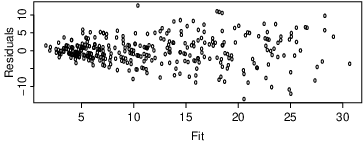
> data(ozone)> res.ibr <- ibr(ozone[,-1],ozone[,1],df=1.1)> summary(res.ibr)Residuals: Min 1Q Median 3Q Max-13.5581 -2.0566 -0.3481 1.9816 12.6049Residual standard error: 3.946 on 309.6 degrees of freedomInitial df: 2.06 ; Final df: 20.42 gcv2.873Number of iterations: 64 chosen by gcvBase smoother: gaussian kernel (with 2.06 df)From the summary, we see that the optimal number of iterations is , which can be thought as quite low (recall that in the previous example the number of iterations ranged between and ). In this example, an exhaustive search method for determining the optimal number of iterations
> ibr(ozone[,-1],ozone[,1],df=1.1,control.par=list(exhaustive=TRUE))gives the same result. Because we only need a relatively small number of bias correction steps, we can select a smaller initial effective degree of freedom, say , while maintaining the computational complexity at a manageable level. Indeed, decreasing the effective degree of freedom of the pilot smoother increases the total number of bias reduction steps while typically providing some performance gains as measured by out of sample prediction errors.
A plot method is also available for the ibr object to display the residuals as a function of the index.
> plot(res.ibr)
To emulate (Bühlmann and Yu, 2003, see) and draw random splits of the data into a set of training data and a set of testing data, we issue the following commands
> XX <- ozone[,-1]> Y <- ozone[,1]> erreur1.5 <- rep(0,33*50)> aa <- c(1,945095059,162152953)> for(i in 1:50){+ set.seed(aa+i)+ ind <- sample(1:330,33)+ XXA <- XX[-ind,]+ YA <- Y[-ind]+ XXT <- XX[ind,]+ YT <- Y[ind]+ res.ibr <- ibr(XXA,YA)+ erreur1.5[(33*(i-1)+1):(33*i)] <- YT-predict(res.ibr,XXT)+ }> print(mean(erreur1.5^2))We get an error of , which compare favorably with GAM (mgcv: 17.44), MARS (mda: 17.49), projection pursuit (ppr: 17.79 for nterms=2) or boosting (package mboost: 17.23). Note that since no default is available for the nterms argument of the function ppr, we follow the examples provided in the ppr documentation and have set nterms equal to 2. To summarize, the ibr smoother enjoys a 15% reduction in the out of sample prediction mean squared error over other state-of-the-art multivariate smoothing methods.
We note that the above comparison favors the boosting and MARS algorithms that take advantage of built-in variable selection procedures. To compare to these methods, we apply the forward variable selection using the random splitting method to ibr for this data set issuing the following commands.
> aa <- c(1,945095059,162152953)> i <- 1> set.seed(aa+i)> ind <- sample(1:330,33)> XXA <- XX[-ind,]> YA <- Y[-ind]> XXT <- XX[ind,]> YT <- Y[ind]We select variables using the commands
> forward.ibr <- forward(XXA,YA)> varnumber <- apply(forward.ibr,1,which.min)> varnumber[1] 4 3 7 6 5That is, the order of the variables to be included into the model is 4, 3, 7, 6 and 5. Variable selection leads to improved predictions. To quantify, on the testing set, this improvement, we compare the the prediction MSE of the selected five variable model with the prediction MSE of model that uses all the eight variables.
> res.ibr <- ibr(XXA,YA)> mean((YT-predict(res.ibr,XXT))^2)[1] 22.90836> res.ibr2 <- ibr(XXA[,varnumber],YA)> mean((YT-predict(res.ibr2,XXT[,varnumber]))^2)[1] 21.12792This shows a small improvement. In conclusion for this example, we remark that despite the increased computational time, the forward function provides simple and useful tool for selecting variables.
5 Conclusion
The ibr package provides additional features which are not offered by other packages on CRAN. These features are a complete implementation, using R language, of iterative biased reduction procedure which implement and generalize the twicing idea of Tukey (1977).
This method of smoothing for multivariate dataset seems to be promising especially on real dataset. But one limitation of this smoothing method is the use of matrix , where is the number of observations. Moreover, at the present time, the computational bottleneck is the eigen decomposition of an matrix, which limits the size of the dataset to which this procedure can be applied too.
References
- Akaike [1973] H. Akaike. Information theory and an extension of the maximum likelihood principle. In B. N. Petrov and B. F. Csaki, editors, Second international symposium on information theory, pages 267–281, Budapest, 1973. Academiai Kiado.
- Antoniadis and Oppenheim [1995] A. Antoniadis and G. Oppenheim. Wavelets in Statistics. Lecture Notes in Statistics, Springer Verlag, 1995.
- Breiman [1996] L. Breiman. Bagging predictors. Machine Learning, 24:123–140, 1996.
- Breiman [1999] L. Breiman. Using adaptive bagging to debias regressions. Technical Report 547, Department of Statistics, UC Berkeley, 1999.
- Bühlmann and Hothorn [2007] P. Bühlmann and T. Hothorn. Boosting algorithms: regularization, prediction and model fitting (with discussion). Statistical Science, 22:477–505, 2007.
- Bühlmann and Yu [2003] P. Bühlmann and B. Yu. Boosting with the loss: Regression and classification. J. Amer. Statist. Assoc., 98:324–339, 2003.
- Bühlmann and Yu [2006] P. Bühlmann and B. Yu. Sparse boosting. J. Machine Learning Research, 7:1001–1024, 2006.
- Buja et al. [1989] A. Buja, T. Hastie, and R. Tibshirani. Linear smoothers and additive models. Ann. of Statist., 17:453–510, 1989.
- Cleveland and Devlin [1988] W. Cleveland and S. Devlin. Locally weighted regression : an approach to regression analysis by local fitting. J. Amer. Stat. Ass., 83:596–610, 1988.
- Cornillon et al. [2008] P. A. Cornillon, N. Hengartner, and E. Matzner-Løber. Recursive bias estimation and boosting. Technical report, arXiv, 2008.
- Cornillon et al. [2011] P. A. Cornillon, N. Hengartner, and E. Matzner-Løber. Recursive bias estimation for multivariate regression smoothers. Technical report, arXiv, 2011.
- Craven and Wahba [1979] P. Craven and G. Wahba. Smoothing noisy data with spline functions: Estimating the correct degree of smoothing by the method of generalized cross-validation. Numerical Mathematics, 31:377–403, 1979.
- Di Marzio and Taylor [2008] M. Di Marzio and C. Taylor. On boosting kernel regression. to appear in JSPI, 2008.
- Eubank [1988] R. Eubank. Spline Smoothing and Nonparametric Regression. Marcel Dekker, New-York, 1988.
- Fan and Gijbels [1996] J. Fan and I. Gijbels. Local Polynomial Modeling and Its Application, Theory and Methodologies. Chapman et Hall, New York, 1996.
- for R and enhanced by Martin Maechler [2010] E. H. P. for R and enhanced by Martin Maechler. lokern: Kernel Regression Smoothing with Local or Global Plug-in Bandwidth, 2010. URL http://CRAN.R-project.org/package=lokern. R package version 1.1-2.
- Friedman [2001] J. Friedman. Greedy function approximation: A gradient boosting machine. Ann. Statist., 28(337-407), 2001.
- Friedman et al. [2000] J. Friedman, T. Hastie, and R. Tibshirani. Additive logistic regression: a statistical view of boosting. Ann. of Statist., 28:337–407, 2000.
- Golub and Van Loan [1996] G. H. Golub and C. F. Van Loan. Matrix computations. The Johns Hopkins University Press, 3 edition, 1996.
- Hansen and Yu [2001] M. Hansen and B. Yu. Model selection and minimal description length principle. J. Amer. Statist. Assoc., 96:746–774, 2001.
- Hastie et al. [2011] T. Hastie, R. Tibshirani, F. Leisch, K. Hornik, and B. D. Ripley. mda: Mixture and flexible discriminant analysis, 2011. URL http://CRAN.R-project.org/package=mda. R package version 0.4-2.
- Hastie and Tibshirani [1990] T. J. Hastie and R. J. Tibshirani. Generalized Additive Models. Chapman & Hall, London, 1990.
- Hastie et al. [2001] T. J. Hastie, R. J. Tibshirani, and J. H. Friedman. The elements of statistical learning: data mining, inference and prediction. Springer, New-York, 2001.
- Hothorn et al. [2010] T. Hothorn, P. Buehlmann, T. Kneib, M. Schmid, and B. Hofner. Model-Based Boosting, 2010. URL http://CRAN.R-project.org/package=mboost. R package version 2.0-9.
- Hurvich et al. [1998] C. Hurvich, G. Simonoff, and C. L. Tsai. Smoothing parameter selection in nonparametric regression using and improved akaike information criterion. J. R. Statist. Soc. B, 60:271–294, 1998.
- Nason [2010] G. Nason. wavethresh: Wavelets statistics and transforms., 2010. URL http://CRAN.R-project.org/package=wavethresh. R package version 4.5.
- R Development Core Team [2009] R Development Core Team. R: A Language and Environment for Statistical Computing. Vienna, Austria, 2009. URL http://www.R-project.org/.
- Ridgeway [2000] G. Ridgeway. Additive logistic regression: a statistical view of boosting: Discussion. Ann. of Statist., 28:393–400, 2000.
- Schwarz [1978] G. Schwarz. Estimating the dimension of a model. Annals of statistics, 6:461–464, 1978.
- Simonoff [1996] J. S. Simonoff. Smoothing Methods in Statistics. Springer, New York, 1996.
- Tukey [1977] J. W. Tukey. Exploratory Data Analysis. Addison-Wesley, 1977.
- Wendelberger [1982] J. Wendelberger. Smoothing noisy data with multivariate splines and generalized cross-validation. Ph.D thesis, University of Wisconsin, 1982.
- Wood [2011] S. N. Wood. mgcv: GAMs with GCV/AIC/REML smoothness estimation and GAMMs by PQL, 2011. URL http://CRAN.R-project.org/package=mgcv. R package version 1.7.5.