The Ridge from the BFKL evolution and beyond

The main objective of this paper is to understand the long range rapidity correlations of charged-particle pairs in the azimuthal angle separation between the two particles around the near side $\Delta\varphi\approx 0$, the so-called ridge which has been recently observed at the LHC in $\sqrt{s}=2.76$ TeV Pb+Pb collisions [1] and also in $\sqrt{s}=7$ TeV proton-proton ($pp$) collisions [2]. The CMS collaboration [2] recently reported that the ridge type structure exists in $pp$ collisions at $\sqrt{s}=7$ TeV for high multiplicity $N\geq 90$ event selections. The origin of the ridge in $pp$ collisions at the LHC is not still well understood and it has been a subject of growing interest, see for example Refs. [3, 4, 5]. The ridge was previously seen at RHIC in central Cu+Cu collisions at $\sqrt{s}=62.4$ GeV and in Au+Au collisions at $\sqrt{s}=200$ GeV [6]. The description of nucleus-nucleus ($AA$) collisions is generally more complicated compared to the case of $pp$ collisions. However, given the relative similarity of the observed ridge structure in both $pp$ and $AA$ collisions in terms of multiplicity, transverse momenta and rapidity separations of pairs, it is natural to ask whether the ridge phenomenon has a unique origin and can be understood only by initial-state effects. We recall that the highest multiplicity events per unit rapidity in $pp$ collisions at $\sqrt{s}=7$ TeV is compatible to the one in central Cu+Cu collisions at RHIC.

In high density QCD, we expect large rapidity correlations for produced hadron pairs with the value of their transverse momenta about the gluon saturation scale $Q_{s}$ [7, 8, 3], see also Ref. [9]. At first sight, these correlations should be small at fixed impact parameters. It has been argued [8] that in the color-glass-condensate (CGC) approach [10] there is a source of the long range rapidity correlations which transforms into the azimuthal angle correlations due to the collective flow in the final state. In Ref. [3] it is argued that such mechanism can qualitatively explain the azimuthal angle correlations in proton-proton collisions without a significant flow effect. The issue of the importance of final-state and collective flow effects in the observed ridge structure in $pp$ collisions [2] is still debatable [4], see also Refs. [11, 12].

In this paper we will introduce a new source of long-range azimuthal correlations for the produced charged hadron pairs. We show that the intrinsic long-range rapidity correlations between the produced hadron pairs from two parton showers generate considerable azimuthal angle correlations which do not depend on the interaction in the final state, and because of this, these correlations have the same origin both in $pp$ and $AA$ interactions at high energy. These correlations have no $1/N_{c}$ suppression as one considered in Refs. [8, 3]. Recently Kovner and Lublinsky in a very nice paper [13] put forward a general discussion toward understanding the ridge. We have an additional goal here, like Ref. [13] we shall try in this paper to understand the general feature of the ridge based on very general grounds and will show that the main features of these correlations both in rapidity and emission angle can be simply understood within the BFKL Pomeron calculus [14, 15, 16, 17, 18, 19]. The extension beyond this framework inside the saturation regime will be also discussed.

The paper is organized as follows: In sec II, we introduce our mechanism for the azimuthal correlations and illustrate the main idea within the perturbative framework. In Sec. III, we consider double inclusive gluon production and its correlations within the BFKL Pomeron approach. We show that the azimuthal correlations between produced hadron pairs from two BFKL parton showers have long-range nature and will survive the BFKL leading log-s re-summation. In Sec. IV, we provide estimates of azimuthal correlations in both $pp$ and $AA$ collisions in the BFKL and the saturation regions. As a conclusion, in Sec. V we highlight our main results.

In this section, we show that the long range rapidity correlations in azimuthal angle separation between the hadron pairs can be simply understood in the perturbative QCD approach. In the parton-like language, the Mueller diagram [20] shown in Fig. 1 (right panel) describes the emission of two particles (partons) from two parton showers. One can write the contribution of this diagram to the cross-section of double inclusive gluon production in the following generic form,

$$\frac{d\sigma}{dy_{1}d^{2}\vec{p}_{1}\,dy_{2}d^{2}\vec{p}_{2}}\,\,=\,\,\frac{1}{2}\,\int d^{2}\vec{Q}_{T}\,N_{{I\!\!P}h}^{2}(Q_{T}^{2})\,\frac{d\sigma}{dy_{1}d^{2}\vec{p}_{1}}\left(\vec{Q}_{T}\right)\,\frac{d\sigma}{dy_{2}d^{2}\vec{p}_{2}}\left(-\vec{Q}_{T}\right),$$

(1)

where $N_{{I\!\!P}h}$ is the scattering amplitudes for Pomeron (ladder)-hadron productions along which transverse momentum $\vec{Q}_{T}$ is transferred and $d\sigma/dy_{i}d^{2}\vec{p}_{iT}$ denotes the corresponding cross-section of the gluon production with rapidity $y_{i}$ and $\vec{p}_{iT}$ in each of the BFKL Pomeron ladders. This factorization is based on the leading Log-s approximation ignoring enhanced Pomeron diagrams. Eq. (1) can be motivated [21, 22, 23, 24, 25] using three main ingredients: Gribov Reggeon [21, 22] and Pomeron [14, 15, 16, 17, 18] calculus, AGK cutting rules [26] and Mueller generalized optical theorem [20]. In the Pomeron calculus the amplitude $N_{{I\!\!P}h}$ is a new ingredient which can be written in the following form,

$$N_{{I\!\!P}h}\left(Q_{T}\right)\,\,=\,\,\sum^{M_{max}}_{n=1}\,g^{2}_{{I\!\!P}n}\left(Q_{T}\right)\,\,+\,\,\int^{\infty}_{M_{max}}\frac{dM^{2}}{M^{2}}\,g_{{I\!\!P}p}\left(Q_{T}=0\right)\,G_{3{I\!\!P}}\left(Q_{T}\right)\,\,\left(M^{2}/s_{0}\right)^{-\Delta_{I\!\!P}}+\dots,$$

(2)

where $n$ denotes the number of produced state with mass $M_{n}$ in the diffractive dissociation with $M_{max}$ as its maximum value (about $2$ GeV) by which one can still express $N_{{I\!\!P}}$ as a sum of resonances, $g_{{I\!\!P}n}$ denotes the vertex of the Pomeron with this state ($g_{{I\!\!P}n}=g_{{I\!\!P}p}$ for $n=1$) and $G_{3{I\!\!P}}$ denotes triple Pomeron vertex. The first term in Eq. (2) describe the contribution of the state with finite mass and this sum can be approximated by the sum of produced resonances. The second term is responsible for high mass contribution and can be described by the Pomeron contribution which leads to the factor $\left(M^{2}/s_{0}\right)^{-\Delta_{I\!\!P}}$ where $\Delta_{I\!\!P}$ is the Pomeron intercept and $s_{0}$ is the energy scale ($s_{0}\approx 1\,\text{GeV}$) [25], see Fig. 2. In the framework of the high energy Pomeron phenomenology it turns out that $Q_{T}$ dependence of the resonance contribution is much steeper than the one in the triple Pomeron term. In the BFKL Pomeron calculus this fact has a natural explanation: the resonance contributions are determined by the non-perturbative soft scale which is about 1 fm, while the triple BFKL Pomeron vertex has a natural scale of the order of the saturation scale which increases with energy. It should be stressed that $N_{{I\!\!P}h}$ has a very simple physical meaning, namely $N_{{I\!\!P}h}^{2}$ is the probability to produce two parton-showers in hadron-hadron collisions.

At first sight, one may expect that Fig. 1 describes two independent parton showers, and therefore there should not be any correlation between two produced gluons from these two parton showers. However, angular correlations stem from the $\vec{Q}_{T}$ integration in Eq. (1). Due to this integration the contribution of diagram in Fig. 1 is not equal to the product of two single inclusive cross-sections leading to nonzero two particle correlation $\mathcal{R}\neq 0$. In order to illustrate this simple fact, let us for the sake of argument assume that the gluon production cross-section in one parton shower is proportional to $\vec{Q}_{T}\cdot\vec{p}_{i,T}$, or in other words,

$$\frac{d\sigma}{dy_{i}d^{2}\vec{p}_{i}}(Q_{T})\propto\vec{Q}_{T}\cdot\vec{p}_{i,T}\frac{d\tilde{\sigma}}{d^{2}y_{i}d^{2}\vec{p}_{i}}.$$

(3)

In this case, Eq. (1) simply becomes

	$\displaystyle\frac{d\sigma}{dy_{1}d^{2}\vec{p}_{1,T}\,dy_{2}d^{2}\vec{p}_{2,T}}\,\,$	$\displaystyle\propto$	$\displaystyle\,\,\int d^{2}\vec{Q}_{T}\,N_{{I\!\!P}h}^{2}(Q^{2}_{T})\,\frac{d\tilde{\sigma}}{dy_{1}d^{2}\vec{p}_{1,T}}\left(Q^{2}_{T}\right)\,\frac{d\tilde{\sigma}}{dy_{2}d^{2}\vec{p}_{2,T}}\left(Q^{2}_{T}\right)\left(\vec{Q}_{T}\cdot\vec{p}_{1,T}\right)\,\left(\vec{Q}_{T}\cdot\vec{p}_{2,T}\right),$		(4)
		$\displaystyle=$	$\displaystyle-\,\vec{p}_{1,T}\cdot\vec{p}_{2,T}\,(\pi/2)\int dQ^{2}_{T}\,N_{{I\!\!P}h}^{2}(Q^{2}_{T})\,\frac{d\tilde{\sigma}}{dy_{1}d^{2}\vec{p}_{1,T}}\left(Q^{2}_{T}\right)\,\frac{d\tilde{\sigma}}{dy_{2}d^{2}\vec{p}_{2,T}}\left(Q^{2}_{T}\right).$

The above equation explicitly shows an angular correlation between two produced gluons in two parton showers. Having this equation in mind, in the next section we will explicitly show that the vertex emission of gluon from the BFKL Pomeron with $Q_{T}\neq 0$ (see Fig. 3) have a structure similar to Eq. (4).

For simplicity and clarity of the presentation, let us first work in the Born approximation, see Fig. 3-a. In this approximation up to $\alpha^{3}$ strong-coupling corrections, the inclusive singlet gluon production at very high energy, assuming that all components of the exchanged momentum are much smaller than the projectile and target momentum (for $s>>\mid t\mid$), is given by

$\displaystyle\frac{d^{2}\sigma}{dy\,d^{2}\vec{p}_{T}}\,\,$

$\displaystyle=$

$\displaystyle\,\,\frac{2\alpha^{3}C_{F}}{\pi^{2}}\int d^{2}\vec{q}_{T}\,\frac{\Gamma_{\mu}\left(\vec{q}_{T},\vec{q^{\prime}}_{T}\right)\,\tilde{\Gamma}^{\mu}\left(-(\vec{q}-\vec{Q})_{T},-(\vec{q^{\prime}}-\vec{Q})_{T}\right)}{q^{2}_{T}\,(\vec{Q}-\vec{q})^{2}_{T}\,q^{\prime 2}_{T}\,(\vec{Q}-\vec{q^{\prime}})^{2}_{T}}\,\,\,,$

(5)

where $C_{F}=(N^{2}_{c}-1)/2N_{c}$ is the $SU(N_{c})$ Casimir operator in the fundamental representation with the number of color equals $N_{c}$. We used a notation $\vec{p}_{T}\,=\,\vec{q}_{T}-\vec{q^{\prime}}_{T}$. The effective vertex $\Gamma_{\mu}$ and $\tilde{\Gamma}_{\mu}$ for the emission of gluons (see Fig. 3-a) are related to the Lipatov vertex $\Gamma_{\mu\nu}^{\rho}$ [14, 15] in the following way,

$$\tilde{\Gamma}^{\rho}\left(\vec{q}_{T},\vec{q^{\prime}}_{T}\right)\,\,=\frac{2}{s}p_{1\mu}p_{2\nu}\Gamma_{\mu\nu}^{\rho}\left(\vec{q}_{T},\vec{q^{\prime}}_{T}\right),$$

(6)

where $p_{1}$ and $p_{2}$ represent the momenta of the incoming projectile and target gluon, and the center of mass energy is $s=2\vec{p}_{1}.\vec{p}_{2}$. The product of the two vertices appeared in Eq. (5) can be simplified to,

	$\displaystyle K\Big(\vec{Q}_{T};\vec{q}_{T},\vec{q^{\prime}}_{T}\Big)\,\,$	$\displaystyle\equiv$	$\displaystyle\,\,\frac{1}{2}\Gamma_{\mu}\left(\vec{q^{\prime}}_{T},\vec{q}_{T}\right)\,\tilde{\Gamma}^{\mu}\left(-(\vec{q}-\vec{Q})_{T},-(\vec{q^{\prime}}-\vec{Q})_{T}\right)\,\,,$		(7)
		$\displaystyle=$	$\displaystyle\,\frac{1}{p^{2}_{T}}\,\Big(q^{\prime 2}_{T}(\vec{Q}-\vec{q})^{2}_{T}\,\,+\,\,q^{2}_{T}\,(\vec{Q}-\vec{q^{\prime}})^{2}_{T}\,\,-\,\,p^{2}_{T}\,Q^{2}_{T}\Big).$

Substituting the above expression into the cross-section Eq. (5), one immediately obtains

	$\displaystyle\frac{d^{2}\sigma}{dy\,d^{2}\vec{p}_{T}}$	$\displaystyle\propto$	$\displaystyle\,\,\alpha^{3}\,\int\frac{d^{2}\vec{q}_{T}}{p^{2}_{T}}\,\Big(\frac{1}{q^{\prime 2}_{T}\,(\vec{Q}-\vec{q})^{2}_{T}}\,\,+\,\,\frac{1}{q^{2}_{T}\,(\vec{Q}-\vec{q^{\prime}})^{2}_{T}}\,\,-\,\,\frac{Q^{2}_{T}p^{2}_{T}}{q^{2}_{T}\,q^{\prime 2}_{T}\,(\vec{Q}-\vec{q})^{2}_{T}\,(\vec{Q}-\vec{q^{\prime}})^{2}_{T}}\Big),$		(8)
		$\displaystyle\xrightarrow{p_{T}\,\ll\,q_{T};\,Q_{T}\,\ll\,q_{T}}\,\,\,\,\,$	$\displaystyle\alpha^{3}\,\int\,\frac{d^{2}\,\vec{q}_{T}}{p^{2}_{T}\,q^{4}_{T}}\,\,\Big\{2\,\,+\,\,4\,\frac{\vec{Q}_{T}\cdot\vec{p}_{T}}{q^{2}_{T}}\,\,+\,\,32\frac{\left(\vec{p}_{T}\cdot\vec{Q}_{T}\right)^{2}}{q^{4}_{T}}\Big\}\,,$		(9)
		$\displaystyle\xrightarrow{p_{T}\,\gg\,q_{T};\,Q_{T}\,\ll\,q_{T}}\,\,\,\,\,$	$\displaystyle\alpha^{3}\,\int\frac{d^{2}\vec{q}_{T}}{q^{2}_{T}\,p^{4}_{T}}\,\Big\{2\,\,+\,\,2\frac{\vec{Q}_{T}\cdot\vec{p}_{T}}{p^{2}_{T}}\,\,+\,\,4\,\frac{\left(\vec{p}_{T}\cdot\vec{Q}_{T}\right)^{2}}{p^{4}_{T}}\Big\}.$		(10)

Notice that in the Born approximation we do not consider the kinematic region $q_{T}\,\ll\,Q_{T}$ since we will show later that this region is not important for the azimuthal correlations from the BFKL Pomeron. Moreover, we should stress that the expansion here are only for the purpose of illustration to trace back the origin of the azimuthal angle correlations in our approach while for the practical estimates, one has to perform the integrals without resorting to any approximation.

First notice that Eq. (5) is symmetric¹¹ 1 We thank our referee for drawing our attention to this point. under $\vec{q}_{T}\to\vec{q^{\prime}}_{T}$ and $\vec{p}_{T}\to-\vec{p}_{T}$. In the expansion given in Eqs. (9,10), we changed the variable to $\vec{q^{\prime}}_{T}\,=\,\vec{q}_{T}\,-\,\vec{p}_{T}$. Changing the variable in Eq. (8) to $\vec{q}_{T}\,=\,\vec{q^{\prime}}_{T}\,+\,\vec{p}_{T}$ and then in the same fashion expanding we get the same expression as in the above equations but the second term in Eqs. (9,10) will be with the opposite sign. Actually, these two expansions correspond to different regions of integrand in Eq. (8). Summing these two contributions²² 2 These two expansions can be also envisaged as two different processes: in Eqs. (9,10) the transverse momentum of produced gluon is compensated by the gluon with the value of the rapidity smaller than the rapidity of the produced gluon with the transverse momentum $p_{T}$ (gluon with rapidity 0 in Fig. 3-a), while expansion in $q^{\prime}_{T}$ we consider the process where $p_{T}$ is balanced by the gluon with the rapidity larger than the rapidity of the produced gluon with the transverse momentum $p_{T}$ (gluon with rapidity $Y$ in Fig. 3-a). we obtain the following form for the double inclusive cross-section from Eq. (1) in the case of $\vec{p}_{T}\,\ll\,\vec{q}_{T},\vec{q^{\prime}}_{T};\,\vec{Q}_{T}\,\ll\,\vec{q^{\prime}}_{T},\vec{q}_{T}$,

	$\displaystyle\frac{d\sigma}{dy_{1}\,dy_{2}\,d^{2}\vec{p}_{1,T}\,d^{2}\vec{p}_{2,T}}\,\,=\,\,\int d^{2}\vec{Q}_{T}N_{{I\!\!P}h}^{2}\left(Q_{T}\right)\,\frac{d\sigma}{dy_{1}\,d^{2}\vec{p}_{1,T}}\left(Q_{T}=0\right)\,\frac{d\sigma}{dy_{2}\,d^{2}\vec{p}_{2,T}}\left(Q_{T}=0\right)\,\,$
	$\displaystyle+\,\,32~p^{2}_{1,T}p^{2}_{2,T}\left(2\,+\,\cos\left(2\Delta\varphi\right)\right)\int d^{2}\vec{Q}_{T}\,Q^{4}_{T}\,N_{{I\!\!P}h}^{2}\left(Q_{T}\right)\,\frac{d\tilde{\sigma}}{dy_{1}\,d^{2}\vec{p}_{1,T}}\left(Q_{T}=0\right)\,\frac{d\tilde{\sigma}}{dy_{2}\,d^{2}\vec{p}_{2,T}}\left(Q_{T}=0\right),$

where $\Delta\varphi$ denotes the angle between $\vec{p}_{1,T}$ and $\vec{p}_{2,T}$ and we defined

$$\frac{d\sigma}{dyd^{2}\vec{p}_{T}}\,\,=\,\,4\frac{2\alpha_{s}}{C_{F}}\,\frac{1}{p_{T}^{2}}\,\int\,d^{2}\vec{q}_{T}\phi\left(\vec{q}_{T},-\vec{q}_{T}\right)\,\phi\left(\vec{q}_{T}-\vec{p}_{T},\vec{p}_{T}-\vec{q}_{T}\right),$$

(12)

and

$$\frac{d\tilde{\sigma}}{dyd^{2}\vec{p}_{T}}\,\,=\,\,4\frac{2\alpha_{s}}{C_{F}}\,\frac{1}{p_{T}^{2}}\,\int\,\frac{d^{2}\vec{q}_{T}}{q^{4}_{T}}\phi\left(\vec{q}_{T},-\vec{q}_{T}\right)\,\phi\left(\vec{q}_{T}-\vec{p}_{T},\vec{p}_{T}-\vec{q}_{T}\right)=\langle\frac{1}{q_{T}^{4}}\rangle\frac{d\sigma}{dyd^{2}\vec{p}_{T}}.\$$

(13)

In the above, we used the following notation,

$$\langle\frac{1}{q_{T}^{4}}\rangle=\frac{\int\,\frac{d^{2}\vec{q}_{T}}{q^{4}_{T}}\phi\left(\vec{q}_{T},-\vec{q}_{T}\right)\,\phi\left(\vec{q}_{T}-\vec{p}_{T},\vec{p}_{T}-\vec{q}_{T}\right)}{\int\,d^{2}\vec{q}_{T}\phi\left(\vec{q}_{T},-\vec{q}_{T}\right)\,\phi\left(\vec{q}_{T}-\vec{p}_{T},\vec{p}_{T}-\vec{q}_{T}\right)},$$

(14)

where $\phi$ denotes the unintegrated gluon density of the projectiles [27] for $Q_{T}=0$,

$$\phi\left(\vec{q}_{T},-\vec{q}_{T}\right)\,\,=\,\,\frac{\alpha_{s}\,C_{F}}{\pi}\,\frac{1}{q^{2}_{T}}.$$

(15)

Notice that at $Q=0$ the inclusive cross-section given in Eq. (5) is identical to Eq. (12).

This simple example indicates that we have a natural mechanism for the azimuthal correlations in the framework of perturbative QCD which does not depend on the final state interactions and leads to the correlations inside of initial wave-function of the incoming hadrons. In the next section, we will show that this azimuthal correlation has long-range nature and will survive the BFKL leading log-s resummation.

The generalization of the Born approximation to the case of gluon emissions from the BFKL Pomeron cannot be simply obtained via Eq. (II) by replacing the unintegrated gluon density $\phi$ to the one obtained from the BFKL equation. Indeed, the unintegrated gluon density $\phi$ depends also on $\vec{Q}_{T}$ and we have to be very careful with putting $Q_{T}=0$. The inclusive gluon product can be generally written as

$$\frac{d\sigma\left(Q_{T}\right)}{dyd^{2}\vec{p}_{T}}\,\,=\,\,4\frac{2\alpha_{s}}{C_{F}}\,\int d^{2}\vec{q}_{T}\,K\Big(\vec{Q}_{T};\vec{q}_{T},\vec{q^{\prime}}_{T}\Big)\,\frac{1}{q^{\prime 2}_{T}\,(\vec{Q}-\vec{q})^{2}_{T}}\,\phi\left(Y-y,\vec{q}_{T},\vec{Q}_{T}-\vec{q}_{T}\right)\,\phi\left(y,\vec{q}_{T}-\vec{p}_{T},\vec{Q}_{T}-\vec{q}_{T}+\vec{p}_{T}\right),$$

(16)

where $K\Big(\vec{Q}_{T};\vec{q}_{T},\vec{q^{\prime}}_{T}\Big)$ is the BFKL kernel given in Eq. (7) and we defined $\vec{q^{\prime}}_{T}=\vec{q}_{T}-\vec{p}_{T}$. In the above, the variable $Y=\ln(s/m^{2})$ denotes the total rapidity in the lab frame where $m$ is the nucleon mass and $y$ and $\vec{p}_{T}$ are the transverse momentum and rapidity of the produced gluon, respectively. Notice that at $Q_{T}=0$, the above expression has the same functional form as the $k_{T}$ factorization [27]. The only dependence on $\vec{p}_{T}$ comes from the term $\phi\left(\vec{q}_{T}-\vec{p}_{T},\vec{Q}_{T}-\vec{q}_{T}+\vec{p}_{T}\right)$ for which we have the color-singlet BFKL equation [14, 28]:

	$\displaystyle\phi\left(y,\vec{q^{\prime}}_{T},\vec{Q}_{T}-\vec{q}^{\prime}_{T}\right)\,\,$	$\displaystyle=$	$\displaystyle\,\,\frac{\bar{\alpha}_{s}}{\pi}\,\int^{y}dy_{i+1}\Big\{\int d^{2}\vec{q^{\prime\prime}}\,K\Big(\vec{Q}_{T};\vec{q^{\prime}}_{T},\vec{q^{\prime\prime}}_{T}\Big)\,\frac{1}{q^{\prime\prime 2}_{T}\,(\vec{Q}-\vec{q^{\prime}})^{2}_{T}}\,\phi\left(y_{i+1},\vec{q^{\prime\prime}}_{T},\vec{Q}_{T}-\vec{q^{\prime\prime}}_{T}\right)\,$		(17)
		$\displaystyle-$	$\displaystyle\,\Big(\frac{q^{\prime 2}_{T}}{(q^{\prime\prime})_{T}^{2}\,(\vec{q^{\prime}}-\vec{q^{\prime\prime}})^{2}_{T}}\,\,+\,\,\frac{(\vec{Q}-\vec{q^{\prime}})^{2}_{T}}{(q^{\prime\prime})_{T}^{2}\,(\vec{Q}-\vec{q^{\prime}}-\vec{q^{\prime\prime}})^{2}_{T}}\Big)\,\phi\left(y_{i+1},\vec{q^{\prime}}_{T},\vec{Q}_{T}-\vec{q}^{\prime}_{T}\right)\Big\},$

where we defined $\bar{\alpha}_{s}=\alpha N_{c}/\pi$. We first substitute $\phi\left(y,\vec{q^{\prime}}_{T},\vec{Q}_{T}-\vec{q}^{\prime}_{T}\right)$ given in Eq. (17) into Eq. (16) and expand the kernels of both equations up to the terms of the order of $Q^{2}_{T}$. Then we again use Eq. (17) but at $Q_{T}=0$ and collect all terms into $\phi\left(y,\vec{q^{\prime}}_{T},\vec{q}^{\prime}_{T}\right)$. Therefore, we obtain the following equation,

	$\displaystyle\frac{d\tilde{\sigma}\left(Q_{T}\right)}{dyd^{2}\vec{p}_{T}}\,\,$	$\displaystyle=$	$\displaystyle\,\,4\frac{\pi\alpha_{s}}{C_{F}}\,\int dq^{2}_{T}\,K\Big(0;\vec{q}_{T},\vec{q^{\prime}}_{T}\Big)\,\frac{1}{q^{\prime 2}_{T}q^{2}_{T}}\,\phi\left(Y,\vec{q}_{T},-\vec{q}_{T}\right)\,\phi\left(y,\vec{q^{\prime}}_{T},-\vec{q^{\prime}}_{T}\right)\Big\{1+\frac{\vec{p}_{T}\cdot\vec{Q}_{T}}{q^{\prime 2}_{T}}+2\frac{\left(\vec{p}_{T}\cdot\vec{Q}_{T}\right)^{2}}{q^{\prime 4}_{T}}\,$		(18)
		$\displaystyle+$	$\displaystyle\dots+\mbox{ terms of the order of $Q_{T}$ that do not lead to azimuthal angle correlations}\Big\}.$

In order to understand better if the above approximation can be justified, let us examine the ladder summations which leads to the BFKL equation. At leading log-s approximation, the imaginary amplitude $\mathcal{A}$ of the quark-quark elastic scattering with exchange of a color-singlet gluon ladder whose vertical lines are reggeized gluons [14, 15, 28] can be written as

$$\text{Im}\mathcal{A}\equiv\sum_{n}\mathcal{A}\left(2\to n\right)\bigotimes\,\mathcal{A}^{*}\left(2\to n\right)=s^{2}C_{F}g_{s}^{4}\sum_{n}\int\prod_{i=0}\frac{g_{s}^{2}K\Big(\vec{Q}_{T},\vec{q}_{i,T},\vec{q}_{i+1,T}\Big)}{\vec{q}_{i+1,T}^{2}(\vec{q}_{i+1,T}-\vec{Q}_{T})^{2}}\left(\frac{\beta_{i}}{\beta_{i+1}}\right)^{\epsilon_{G}\left(\vec{q}_{i+1,T}\right)+\epsilon_{G}\left(\vec{q}_{i+1,T}-\vec{Q}_{T}\right)},$$

(19)

where $K\Big(\vec{Q}_{T},\vec{q},\vec{q^{\prime}}\Big)$ is again the BFKL kernel given in Eq. (17). The right-hand side of the above equation shows that the BFKL Pomeron can be written as a sum of production cross-sections as it follows from the optical theorem. The symbol $\bigotimes$ denotes the integrations over $n+2$-body phase space and the parameters $\beta_{i}$ (with $\beta_{0}=1$) is the standard Sudakov variables for the momentum of the $t$-channel gluons which obeys strong ordering of the longitudinal momenta [14, 15, 28]. The expression in Eq. (19) takes into account the reggeization of gluons in $t$-channel that means that the spin of the gluon is not equal to $1$ as in perturbative calculations but it is given by the reggeized gluon trajectory

$$\alpha_{G}\left(\vec{q}_{i,T}\right)\,\,=1+\epsilon_{G}(\vec{q}_{i,T})=\,\,1\,\,+\,\,\frac{\bar{\alpha}_{s}}{\pi}\int\frac{d^{2}\vec{q^{\prime}}_{T}q^{2}_{i,T}}{q^{\prime 2}_{T}\,(\vec{q}_{i,T}-\vec{q^{\prime}}_{T})^{2}}.$$

(20)

We recall that the produced gluon in the $i$th rung ladder is on-shell with $\vec{p}_{i,T}=\vec{q}_{i+1,T}-\vec{q}_{i,T}$. Then, in order to find $\vec{Q}_{T}$ and $\vec{p}_{i,T}$ correlations one needs only to keep $Q_{T}\neq 0$ in the $i$th rung of the ladder (see Fig. 3-b ) and to put $Q_{T}=0$ in all other rungs. The contribution of this particular sell to the amplitude has the following structure

			$\displaystyle\frac{K\Big(\vec{Q}_{T},\vec{q}_{i,T},\vec{q}_{i+1,T}\Big)}{(\vec{q}_{i+1,T}-\vec{p}_{i})^{2}(\vec{q}_{i+1,T}-\vec{p}_{i}-\vec{Q}_{T})^{2}q_{i+1,T}^{2}(\vec{q}_{i+1,T}-\vec{Q}_{T})^{2}}$		(21)
		$\displaystyle\times$	$\displaystyle\left(\frac{\beta_{i}}{\beta_{i+1}}\right)^{\epsilon_{G}\left(\vec{q}_{i+1,T}\right)+\epsilon_{G}\left(\vec{q}_{i+1,T}-\vec{Q}_{T}\right)}\left(\frac{\beta_{i-1}}{\beta_{i}}\right)^{\epsilon_{G}\left(\vec{q}_{i+1,T}-\vec{p}_{i}\right)+\epsilon_{G}\left(\vec{q}_{i+1,T}-\vec{p}_{i}-\vec{Q}_{T}\right)}.\$

Although the above equation includes the virtual radiative corrections, but has a very similar structure to the case of the Born approximation given in Eq. (5) and consequently in the same fashion discussed in the previous section, it also gives rise to the azimuthal correlations. Therefore, in order to extract the correlations between two produced gluons, it is sufficient to use Eq. (17) in which we can put $Q_{T}=0$ in $\phi\left(\vec{q^{\prime\prime}}_{T},\vec{Q}_{T}-\vec{q^{\prime\prime}}_{T}\right)$ and $\phi\left(q^{\prime}_{T},\vec{Q}_{T}-\vec{q^{\prime}}_{T}\right)$. Using Eq. (18) and adding the contribution of the integration region in $q_{T}$ where $|\vec{q}_{T}-\vec{p}_{T}|\,\gg\,|\vec{p}_{T}|$, we obtain from Eq. (1),

	$\displaystyle\frac{d\sigma}{dy_{1}\,dy_{2}\,d^{2}\vec{p}_{1,T}\,d^{2}\vec{p}_{2,T}}\,\,$	$\displaystyle=$	$\displaystyle\,\,\pi\int dQ^{2}_{T}\,N_{{I\!\!P}h}^{2}(Q^{2}_{T})\,\frac{d\sigma}{dy_{1}\,d^{2}p_{1,T}}\left(Q_{T}=0\right)\,\frac{d\sigma}{dy_{2}\,d^{2}p_{2,T}}\left(Q_{T}=0\right)\,$		(22)
			$\displaystyle\Big\{1\,\,+\,\frac{1}{2}\,p^{2}_{1,T}\,p^{2}_{2,T}\,Q^{4}_{T}\,\langle\frac{1}{q^{4}}\rangle^{2}\,\left(2\,+\,\cos\left(2\Delta\varphi\right)\right)\Big\},$
		$\displaystyle=$	$\displaystyle{\cal N}\,\Big(1\,\,+\,\,\frac{1}{2}\,p^{2}_{1,T}\,p^{2}_{2,T}\,\,\langle\langle Q^{4}_{T}\rangle\rangle\,\langle\frac{1}{q^{4}}\rangle^{2}\left(2\,+\,\cos\left(2\Delta\varphi\right)\right)\Big),$		(23)

where $\Delta\varphi$ is the angle between $\vec{p}_{1,T}$ and $\vec{p}_{2,T}$ and we defined the following notations,

	$\displaystyle\langle\frac{1}{q^{2n}_{T}}\rangle$	$\displaystyle=$	$\displaystyle\frac{\int\frac{d^{2}\vec{q}_{T}}{q^{2n}_{T}}~\phi\left(Y-y,\vec{q}_{T},-\vec{q}_{T}\right)\,\phi\left(y,\vec{q}_{T}-\vec{p}_{T},\vec{p}_{T}-\vec{q}_{T}\right)}{\int d^{2}\vec{q}_{T}\phi\left(Y-y,\vec{q}_{T},-\vec{q}_{T}\right)\,\phi\left(y,\vec{q}_{T}-\vec{p}_{T},\vec{p}_{T}-\vec{q}_{T}\right)},$		(24)
	$\displaystyle\langle\langle Q^{2n}_{T}\rangle\rangle$	$\displaystyle=$	$\displaystyle\frac{\int d^{2}\vec{Q}_{T}~Q^{2n}_{T}\,N_{{I\!\!P}h}^{2}(Q^{2}_{T})}{\int d^{2}\vec{Q}_{T}\,N_{{I\!\!P}h}^{2}(Q^{2}_{T})},$		(25)

with $n=1,2$. The normalization factor $\cal N$ in Eq. (23) is given by

$${\cal N}\,\,\,\equiv\,\,\pi\int dQ^{2}_{T}\,N_{{I\!\!P}h}^{2}(Q^{2}_{T})\,\frac{d\sigma}{dy_{1}\,d^{2}\vec{p}_{1,T}}\left(Q_{T}=0\right)\,\frac{d\sigma}{dy_{2}\,d^{2}\vec{p}_{2,T}}\left(Q_{T}=0\right).$$

(26)

From the above, it is obvious that the production of two parton showers with a transverse momentum $\vec{Q}_{T}$ along the Pomeron ladder, naturally leads to the long range rapidity correlation in azimuthal angle while the emissions from one parton shower given by the BFKL Pomeron contribution does not lead to such correlations, see also Ref. [7].

We recall that the long-range azimuthal angle correlations obtained by Eq. (23) is valid in the leading log-s approximation at high-energy. The azimuthal angle correlations in Eq. (23) is uniquely determined by only knowing the average values $\langle 1/q^{2n}_{T}\rangle$ and $\langle\langle Q^{2n}_{T}\rangle\rangle$. This equation was truncated at $n=2$ assuming that the transverse momentum $Q_{T}$ in the Pomeron ladder is small. Let us explore the idea that Eq. (23) is also valid in the saturation region (or at least on the boundary between the BFKL and the saturation regime) by choosing the corresponding average values $\langle 1/q^{2n}_{T}\rangle$ and $\langle\langle Q^{2n}_{T}\rangle\rangle$ in that region.

In the kinematic regime of the BFKL (ignoring the saturation effect) from Eq. (24) we obtain $\langle 1/q^{2n}_{T}\rangle\,\approx 1/\text{max}\{\mu^{2n},Q_{T}^{2n}\}$ where $\mu$ is the non-perturbative soft scale. At the LHC energies, the inclusive production stems from the kinematic region in which saturation effects are important [29, 30, 31]. In this region, the interaction between Pomerons leads to more complicated diagrams, the so-called enhanced diagrams shown in Fig. 4. It has been shown (see Ref. [19] and references therein) that the enhanced diagram leads to the value of the characteristic momentum of the order of $Q_{s}$, namely we have $Q_{T}\propto Q_{s}$ . We do not need to follow complete calculations of this paper to understand why it happens so. Indeed, assuming that $Q_{T}\,\ll\,\mbox{typical q $\approx Q_{s}$}$ we can replace the BFKL Pomerons in the loop by the Pomerons at $Q_{T}=0$. Therefore, in this case, we have $\int^{Q_{s}}d^{2}Q_{T}\,=\,Q^{2}_{s}$. For $Q_{T}\gg q$ the Pomeron exchange falls down with $Q_{T}$ making the integral being concentrated at $Q_{T}=q_{T}=Q_{s}$. In order words, if densities of partons in one parton shower is so large that we have already reached the saturation region of the gluon density, we can assume that the average $\langle 1/q^{2n}_{T}\rangle\approx 1/Q^{2n}_{s}$ where $Q_{s}$ is the saturation scale. This also follows from the high-density QCD within the CGC approach [10] which describes the LHC data for the inclusive hadron production both in $pp$ and $AA$ collisions [29, 30], see also Ref. [31]. We also assume that the density of partons in both parton showers is very large and consequently Pomeron enhanced diagrams are important, and therefore we can have $\langle\langle Q^{2n}_{T}\rangle\rangle\approx Q^{2n}_{s}$. Therefore, we assume that in the saturation region we have only one relevant scale, the saturation scale, and the average transverse momenta are related to this scale.

Notice that the maximum of the double inclusive production reaches at $p_{1,T}\approx p_{2,T}\approx Q_{s}$. Admittedly, we do not have a rigorous proof of this at our disposal without invoking any approximation, but this may be immediately understood within the CGC approach since $Q_{s}$ is the only dimensional parameter of the approach. This can be also seen in the simple case of the Born approximation by comparing Eqs. (9, 10). Note that Eq. (9) gives the contribution at small values of $p_{T}$ and the correlations vanish at $p_{t}\to 0$ and increase with $p_{T}$ while Eq. (10) shows that the correlations falls down at large values of $p_{T}$. Therefore, the correlation function has a maximum at $p_{T}\approx\langle q_{T}\rangle$, where $\langle q_{T}\rangle$ is the typical transverse momentum of the system. The same argument is valid for the general case of the gluon pairs production from the BFKL Pomeron. This can be seen by comparing Eq. (23) and its corresponding equation in the limit of $p_{T}\gg q_{T}\gg Q_{T}$. It should be stressed that the experimental data from the CMS collaboration indicates that the maximum of correlations occurs at the kinematic region that the saturation effects is important [2].

The probability for the events with multiplicity equals $N=2\langle N\rangle$ where $\langle N\rangle$ is the multiplicity in one parton shower, can be obtained by Eq. (26) and the corresponding cross-section of such events is $\sigma(N=2\langle N\rangle)\propto{\cal N}$. Using Eq. (23), we obtain two-particle correlation function $\mathcal{R}$ for the event selections with multiplicity $N$ as,

$$\mathcal{R}\left(\Delta\varphi;y_{1},y_{2}\right)\,\,=\,\,\frac{\frac{dN}{dy_{1}d^{2}\vec{p}_{1,T}dy_{2}d^{2}\vec{p}_{2,T}}}{\frac{d^{2}N}{dy_{1}d^{2}\vec{p}_{1,T}}\,\frac{d^{2}N}{dy_{2}d^{2}\vec{p}_{2,T}}}\,\,\,-\,\,\,1\,\,=\,\,\frac{\overline{n}(\overline{n}-1)}{2~\overline{n}^{2}}\,\,\Big\{1\,\,+\,\,\frac{1}{2}\,\left(2\,+\,\cos\left(2\Delta\varphi\right)\right)\Big\}\,\,-\,\,1,$$

(27)

where the parameter $\overline{n}=E\left(N/\langle N\rangle\right)$ is the relative average number of Pomeron parton showers in the event selections with multiplicity $N$, the average multiplicity $\langle N\rangle$ denotes the multiplicity in the mini-bias and function $E$ gives the integer value of its argument. The pre-factor in Eq. (27) comes from the counting the various possible ways to have two gluons production out of $\overline{n}$ Pomeron parton showers. In other words, for simplicity we assumed that $\bar{n}$ showers are produced and two correlated gluons comes from only two different parton showers. The number of these pairs is equal to $\bar{n}\left(\bar{n}-1\right)/2$ and moreover we have $\frac{d^{2}N}{dy_{i}d^{2}p_{i,T}}\,\,=\,\,\bar{n}\frac{d^{2}N\left(\mbox{one parton shower}\right)}{dy_{i}d^{2}p_{i,T}}$, therefore the pre-factor in Eq. (27) can be readily obtained.

Notice that the main background for the double inclusive gluons production is due to two jets production from one parton shower. However, this production is suppressed by making selection in the events. From AGK cutting rules [26], it follows that the multiplicity in one parton shower is equal to the average multiplicity measured by the experiment in the mini-bias events. It should be stressed that the AGK cutting rules also work for two parton showers production in QCD [35]. It is well-known that the gluon distribution in the BFKL Pomeron is close to the Poisson distribution, see Ref. [36] and references therein. The production from two parton showers starts to be significant only for the events with multiplicity larger than $2\langle N\rangle$ where $\langle N\rangle$ is the mean multiplicity, see Fig. 1. On the other hand, the probability to have events with multiplicity $2\langle N\rangle$ in one parton shower is approximately suppressed as $\exp\left(-(2\langle N\rangle-\langle N\rangle)^{2}//2\langle N\rangle\right)\,\ll\,1$ for the Poisson distribution.

One can observe in Eq. (27) that except the over-all pre-factor, the coefficients does not depend on multiplicity and rapidity of pairs. Of course this feature may be altered due to possible contamination of two gluons production from one parton shower which may lead to short range rapidity correlations in the azimuthal angle $\Delta\varphi$. However, in particular experimental set up with high multiplicity events where our underlying saturation assumption namely $\langle\langle Q^{2n}_{T}\rangle\rangle\approx\langle q^{2n}_{T}\rangle\approx Q_{s}^{2n}$ is at work, these correlations could be ignored and can only create a back ground that will fall off at large multiplicity events.

In order to understand how much the azimuthal asymmetry depends on the value of $\langle\langle Q^{2n}_{T}\rangle\rangle$, we next estimate $\langle\langle Q^{2n}_{T}\rangle\rangle$ in the BFKL kinematic region ignoring the so-called enhanced diagrams (shown in Fig. 4). In order to calculate $\langle\langle Q^{2n}_{T}\rangle\rangle$ defined in Eq. (25), we should know the non-perturbative amplitude $N_{{I\!\!P}p}\left(Q_{T}\right)$ defined in Eq. (2). For $N_{{I\!\!P}p}\left(Q_{T}\right)$, we use the quasi-eikonal approximation [24]. In this approximation we restrict ourselves to the first term in Eq. (2) and the contribution of the other terms is taken into account by introducing an extra factor $N_{0}$,

$$N_{{I\!\!P}p}\left(Q_{T}\right)\,\,=\,\,N_{0}g^{2}_{{I\!\!P}p}\left(Q_{T}\right),$$

(28)

where $g_{{I\!\!P}p}$ is the vertex of Pomeron-proton interaction. This approximation has been widely employed in Pomeron phenomenology and works quite well in the description of the experimental data [32]. The dependence of the BFKL Pomeron on the transverse momentum $Q_{T}$ is given by $g_{{I\!\!P}p}\left(Q_{T}\right)=1/(1+Q^{2}_{T}/m^{2})^{2}$ with the typical mass $m$ determined from the experimental data. The dipole form of $g_{{I\!\!P}p}$ is inspired by the $Q_{T}$ dependence of the electromagnetic form factor of the proton. Using this distribution we obtain $\langle Q^{2}_{T}\rangle=m^{2}/6$ and $\langle Q^{4}_{T}\rangle=m^{2}/15$. The experimental data for diffractive production of the vector meson in the DIS [33] indicates that $m^{2}=0.8\,\text{GeV}^{2}$. However, the CDF data on double jet production [34] shows that the typical value of $Q_{T}$ could be larger leading to a bigger value for $m^{2}=1.6\,\text{GeV}^{2}$. Again assuming that $\langle q_{T}^{2n}\rangle=Q_{s}^{2n}$ the corresponding two-particle correlation function $\mathcal{R}$ for $p_{1T}=p_{2T}=Q_{s}$ and $\overline{n}\geq 2$ becomes,

$$\mathcal{R}\left(\Delta\varphi;y_{1},y_{2}\right)\,\,\,\,=\frac{\overline{n}(\overline{n}-1)}{2~\overline{n}^{2}}\,\,\Big\{\,\,1\,\,+\,\,\frac{m^{4}}{30\,Q^{4}_{s}}\,\left(2\,+\,\cos\left(2\Delta\varphi\right)\right)\,\,\Big\}-1.$$

(29)

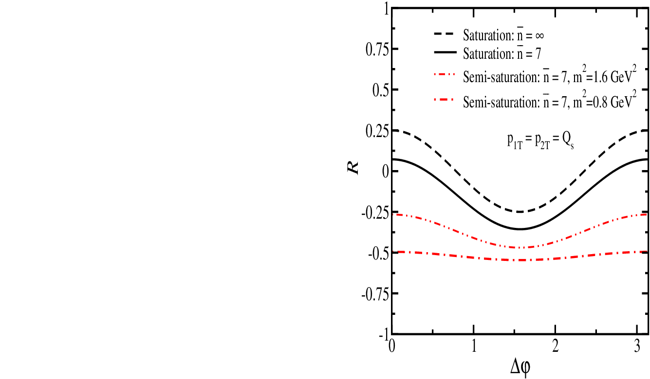
It is seen from above that the coefficients in $\mathcal{R}$ now depends on the rapidity via the saturation scale $Q_{s}$ in contrast to Eq. (27). However, one should note that deep inside the saturation region the above equation is not reliable and one should then use Eq. (27). It is instructive to notice that the two BFKL parton showers contribution lead to Eq. (29) with the soft scale $\mu$ instead of $Q_{s}$. This scale is a new phenomenological parameter which does not depend on energy, and it is certainly $\mu\leq Q_{s}$.

In Fig. 5 (right) we show the azimuthal correlation $\mathcal{R}$ obtained from Eq. (29) when $\langle\langle Q_{T}^{2n}\rangle\rangle$ was calculated within the BFKL region for two different masses $m^{2}=0.8\,\text{GeV}^{2}$ and $m^{2}=1.6\,\text{GeV}^{2}$. In this plot, we take a fixed saturation scale $Q_{s}^{2}=0.6\,\text{GeV}^{2}$. The chosen saturation scale is in accordance with the estimates of Ref. [29] in $pp$ collisions at the LHC. In Fig. 5 (right) we also show the azimuthal correlation $\mathcal{R}$ obtained from Eq. (27) in the saturation region at different multiplicity $N=\overline{n}\langle N\rangle$. It is observed that deep inside the saturation region we have the ridge-type structure, namely a second local maximum near $\Delta\varphi\approx 0$ independent of rapidity when $p_{T}$ is about the saturation scale. By comparing the results shown in Fig. 5 from Eqs. (27,29), it is notably seen that by going from the BFKL to the saturation region, a pronounced ridge-type structure emerges. In Fig. 5 we show the experimental data from the CMS collaboration [2] for projections of two dimensional correlation functions onto $\Delta\varphi$ (denoted in Fig. 5 left panel by $\Delta\phi$) for the difference in pseudorapidity of pair $2<\Delta\eta<4.8$ in different $p_{T}$ and multiplicity bins at 7 TeV pp collisions and reconstructed PYTHIA8 simulations [37]. It is important to note that PYTHIA8 qualitatively fails to reproduce the local maximum in the near-side correlation in any of the $p_{T}$ or multiplicity bins [2], see Fig. 5. Notice that our definition of two-particle correlation $\mathcal{R}$ defined in Eq. (27) is different from the experimental definition $R$ [2] shown in Fig. 5 with a over-all factor. Here given the simplicity of our approach we do not wish to compare directly our results with the experimental data. A meaningful comparison requires inclusion of correlations effect within one parton-shower, fragmentation and possible short-range correlation effects. Nevertheless, it is seen that the general feature of the near-side two-point correlations obtained by Eqs. (27,29) is compatible with the CMS experimental data [2]. One should note that for a denser system, the imposed condition of $p_{1T}=p_{2T}=Q_{s}$ in Eq. (27) shifts the relevant kinematic windows of the angular correlations to the higher $p_{T}$ since the saturation scale will be larger for a denser system.

Next, we consider the long-range correlations in nucleus-nucleus scatterings. It is straightforward to generalize Eq. (22) for the case of nucleus-nucleus collisions in the framework of the Glauber approach, namely assuming that multiple scatterings are only permitted on different nucleons while the nucleon-nucleon scattering stems from the BFKL Pomeron exchange. The double inclusive cross-section at a fixed impact-parameter between two center of nuclei $b$ will then have the same form as Eq. (22) except the extra dependence on the nuclear profile. Notice that the impact-parameter $b$ is the conjugate variable to transverse momentum $Q_{T}$. In the Glauber approximation for nuclei, the scattering amplitude of Pomeron-nucleus $N_{{I\!\!P}A}$ in the region of small diffractive masses is defined as

	$\displaystyle N_{{I\!\!P}A}\left(Q_{T}\right)\,\,$	$\displaystyle\equiv$	$\displaystyle\left(\int\,d^{2}\vec{b}~d^{2}\vec{b^{\prime}}\,e^{i\vec{Q}_{T}\cdot\vec{b}}\,S_{A}\left(\vec{b}-\vec{b^{\prime}}\right)g_{{I\!\!P}p}(\vec{b^{\prime}})\right)^{2},$		(30)
		$\displaystyle\approx$	$\displaystyle~g^{2}_{{I\!\!P}p}(q_{T}=0)~S^{2}_{A}(Q_{T}),\$

where $g_{{I\!\!P}p}$ denotes the Pomeron-proton vertex and $S_{A}\left(b\right)$ is the nuclear density profile defined by the Wood-Saxon parametrization. The second equation above is valid when the nuclear radius is larger compared to the proton size $R_{A}>>R_{p}$. Using Eq. (30) one can obtain the following expression for the double inclusive cross-section at fixed $b$ in the framework of the Glauber approach in which the proton-proton scatterings are taken into account from the BFKL Pomeron:

	$\displaystyle\frac{d\sigma_{A}}{dy_{1}\,dy_{2}\,d^{2}p_{1,T}\,d^{2}p_{2,T}\,d^{2}b}$	$\displaystyle=$	$\displaystyle\frac{1}{2}\,\frac{d\sigma_{N}}{dy_{1}\,d^{2}p_{1,T}}\frac{d\sigma_{N}}{dy_{2}\,d^{2}p_{2,T}}$		(31)
		$\displaystyle\times$	$\displaystyle\Big\{T_{AA}^{2}(b)+\,\frac{1}{2}\,p^{2}_{1,T}\,p^{2}_{2,T}\,\Big(\langle 1/q^{4}\rangle_{\text{proton}}\Big)^{2}\,\Big(\bigtriangledown^{2}_{b}\bigtriangledown^{2}_{b}\,T^{2}_{AA}(b)\Big)\left(2\,+\,\cos\left(2\Delta\varphi\right)\right){\Big\}},\$

where $\frac{d\sigma_{N}}{dy_{1}\,d^{2}p_{1,T}}$ is the inclusive cross-section for proton-proton scatterings ³³ 3 It should be noted that the inclusive cross-section of proton-proton scatterings enters Eq. (31) since the integration over the impact parameter of proton-proton scatterings has been performed as usual in the Glauber approach. and $T_{AA}$ is the nuclear overlap function for AA collisions. Using Eq. (31) one can calculate the correlation function $\mathcal{R}$ defined in Eq. (27):

$\displaystyle\mathcal{R}\left(b,\Delta\varphi,y_{1},y_{2}\right)\,\,$

$\displaystyle=$

$\displaystyle\,\,\,\frac{1}{2}\,p^{2}_{1,T}\,p^{2}_{2,T}\,\Big(\langle 1/q^{4}\rangle_{\text{proton}}\Big)^{2}\,\Big(\bigtriangledown^{2}_{b}\bigtriangledown^{2}_{b}\,T^{2}_{AA}(b)\Big)\left(2\,+\,\cos\left(2\Delta\varphi\right)\right).\$

(32)

It is straightforward to show that in the Glauber approach, the inclusive production in $AA$ collisions is proportional to the overlap function $T_{AA}(b)$ while in the case of the double inclusive production instead it is proportional to $T_{AA}^{2}(b)$. It is seen from Eq. (32) that independent productions are canceled in $\mathcal{R}$ at fixed $b$ while in the integral over $b$ the first term in Eq. (31) gives the main contribution. It is worth mentioning that we do not need additional factor $\overline{n}$ as in Eq. (29) since in the Glauber formulation for nucleus-nucleus scatterings, events with a fixed multiplicity correspond to a definite value of the impact-parameter.

References

- [1] CMS Collaboration, arXiv:1105.2438.
- [2] V. Khachatryan et al. [CMS Collaboration], JHEP 1009 (2010) 091 [arXiv:1009.4122].
- [3] A. Dumitru, K. Dusling, F. Gelis, J. Jalilian-Marian, T. Lappi and R. Venugopalan Phys. Lett. B697 (2011) 21.
- [4] K. Werner, Iu. Karpenko, T. Pierog, Phys. Rev. Lett. 106 (2011) 122004; P. Bozek, arXiv:1010.0405.
- [5] I. O. Cherednikov and N. G. Stefanis, arXiv:1010.4463; Igor M. Dremin, Victor T. Kim, arXiv:1010.0918; S. M. Troshin and N. E. Tyurin, arXiv:1009.5229; I. Bautista, J. Dias de Deus and C. Pajares, e-Print: arXiv:1011.1870; M. Y. Azarkin, I. M. Dremin and A. V. Leonidov, arXiv:1102.3258; M. Diehl and A. Schafer, Phys. Lett. B698 (2011) 389; J. Bartels and M. G. Ryskin, arXiv:1105.1638; S. Vogel, P. B. Gossiaux, K. Werner and J. Aichelin, arXiv:1012.0764; R. C. Hwa and C. B. Yang, Phys. Rev. C83 (2011) 024911; E. Avsar, C. Flensburg, Y. Hatta, J-Y Ollitrault and T. Ueda, arXiv:1009.5643; H. R. Grigoryan and Y. V. Kovchegov, JHEP 1104 (2011) 010.
- [6] J. Adams et al. [STAR Collaboration], Phys. Rev. Lett. 95 (2005) 152301; J. Adams, et al. [STAR Collaboration], Phys. Rev. C73 (2006) 064907; A. Adare et al. [PHENIX Collaboration], Phys. Rev. C78 (2008) 014901; B. I. Abelev et al. [STAR Collaboration], Phys. Rev. C80 (2009) 064912; B. Alver et al. [PHOBOS Collaboration], Phys. Rev. Lett. 104 (2010) 062301.
- [7] Y. V. Kovchegov, E. Levin and L. D. McLerran, Phys. Rev. C63 024903 (2001) [hep-ph/9912367]; D. Kharzeev, E. Levin and L. McLerran, Nucl. Phys. A748 (2005) 627 [hep-ph/0403271]; N. Armesto, L. McLerran and C. Pajares, Nucl. Phys. A781 (2007) 201 [hep-ph/0607345]; K. Fukushima and Y. Hidaka, Nucl. Phys. A813 (2008) 171 [arXiv:0806.2143].
- [8] A. Dumitru, F. Gelis , L. McLerran and R. Venugopalan, Nucl. Phys. A810 (2008) 91 [arXiv:0804.3858]; K. Dusling, F. Gelis, T. Lappi and R. Venugopalan, Nucl. Phys. A836 (2010)159 [arXiv:0911.2720].
- [9] A. Dumitru and J. Jalilian-Marian, Phys. Rev. D81 (2010) 094015 (2010); T. Lappi and L. McLerran, Nucl. Phys. A832 (2010) 330 [arXiv:0909.0428]; F. Gelis, T. Lappi and L. McLerran, Nucl. Phys. A828 (2009) 149 [arXiv:0905.3234]; G. Moschelli, S. Gavin and L. McLerran, Eur. Phys. J. C62 (2009) 277; J. Jalilian-Marian, arXiv:1011.1601; T. Lappi, arXiv:1011.0821.
- [10] L. McLerran and R. Venugopalan, Phys. Rev. D49 (1994) 2233; D49 (1994) 3352; D50, (1994) 2225; D53 (1996) 458; D59 (1999) 094002. For a recent review see: R. Venugopalan, arXiv:1012.4699; L. McLerran, arXiv:1011.3203; F. Gelis, E. Iancu, J. Jalilian- Marian and R. Venugopalan, arXiv:1002.0333.
- [11] D. d’Enterria, G. Kh. Eyyubova, V. L. Korotkikh, I. P. Lokhtin, S. V. Petrushanko, L. I. Sarycheva, A. M. Snigirev, Eur. Phys. J. C66 (2010) 173 [arXiv:0910.3029].
- [12] B. Z. Kopeliovich, A. H. Rezaeian and I. Schmidt, Phys. Rev. D78 (2008) 114009 [arXiv:0809.4327].
- [13] A. Kovner, M. Lublinsky, Phys. Rev. D83 (2011) 034017 [arXiv:1012.3398].
- [14] E. A. Kuraev, L. N. Lipatov, and F. S. Fadin, Sov. Phys. JETP 45 (1977) 199; Ya. Ya. Balitsky and L. N. Lipatov, Sov. J. Nucl. Phys. 28 (1978) 22.
- [15] L. V. Gribov, E. M. Levin and M. G. Ryskin, Phys. Rep. 100 (1983) 1.
- [16] A. H. Mueller and J. Qiu, Nucl. Phys. B268 (1986) 427.
- [17] M. A. Braun, Phys. Lett. B632 (2006) 297 [hep-ph/0512057]; arXiv:hep-ph/0504002 ; Eur. Phys. J. C16 (2000) 337 [hep-ph/0001268]; Phys. Lett. B483 (2000) 115 [hep-ph/0003004]; Eur. Phys. J. C33 (2004) 113 [hep-ph/0309293]; Eur. Phys. J. C6 (1999) 321 [hep-ph/9706373]; M. A. Braun and G. P. Vacca, Eur. Phys. J. C6 (1999) 147 [hep-ph/9711486].
- [18] J. Bartels, M. Braun and G. P. Vacca, Eur. Phys. J. C40 (2005) 419 [arXiv:hep-ph/0412218]; J. Bartels and C. Ewerz, JHEP 9909, 026 (1999) [hep-ph/9908454]; J. Bartels and M. Wusthoff, Z. Phys. C66 (1995) 157, A. H. Mueller and B. Patel, Nucl. Phys. B425 (1994) 471 [hep-ph/9403256]; J. Bartels, Z. Phys. C60 (1993) 471.
- [19] E. Levin, J. Miller and A. Prygarin, Nucl. Phys. A806 (2008) 245.
- [20] A. H. Mueller, Phys. Rev. D2 (1970) 2963.
- [21] P. D. B. Collins, ”An introduction to Regge theory and high energy physics”, Cambridge University Press 1977.
- [22] L. Caneschi (editor), ”Regge Theory of Low - Hadronic Interaction”, North-Holland 1989.
- [23] E. M. Levin, M. G. Ryskin and N. N. Nikolaev, Z. Phys. C5 (1980) 285; E. M. Levin, M. G. Ryskin and S. I. Troian, Sov. J. Nucl. Phys. 23 (1976) 222 [Yad. Fiz. 23 (1976) 423]; E. M. Levin and M. G. Ryskin, Sov. J. Nucl. Phys. 20 (1975) 280 [Yad. Fiz. 20 (1974) 519]; E. L. Berger and M. Jacob, Phys. Rev. D6 (1972) 1930.
- [24] A. B. Kaidalov and K. A. Ter-Martirosian, Sov. J. Nucl. Phys. 39 (1984) 979 [Yad. Fiz. 39 (1984) 1545]; A. B. Kaidalov, Phys. Rept. 50 (1979) 157.
- [25] P. Aurenche, F. W. Bopp, A. Capella, J. Kwiecinski, M. Maire, J. Ranft and J. Tran Thanh Van, Phys. Rev. D45 (1992) 92; F. W. Bopp, A. Capella, J. Ranft and J. Tran Thanh Van, Z. Phys. C51 (1991) 99; A. Capella, C. Pajares and A. V. Ramallo, Nucl. Phys. B241 (1984) 75; A. Capella and J. Tran Thanh Van, Phys. Rev. D29 (1984) 2512; Ȧ. Capella and J. Tran Thanh Van Z. Phys. C18 (1983) 85; A. Capella and A. Krzywicki, Phys. Rev. D18 (1978) 4120; A. Capella, U. Sukhatme, C. I. Tan and J. Tran Thanh Van, Phys. Rept. 236 (1994) 225.
- [26] V. A. Abramovsky, V. N. Gribov, O. V. Kancheli, Yad. Fiz. 18 (1973) 595 [Can be found in Ref. [22]].
- [27] Y. V. Kovchegov and K. Tuchin,Phys. Rev. D65 (2002) 074026. Y. V. Kovchegov, Phys. Rev. D72 (2005) 094009.
- [28] E. M. Levin and M. G. Ryskin, Phys. Rept. 189 (1990) 267 ; L. N. Lipatov, Phys. Rept. 286 (1997) 131 and references therein.
- [29] E. Levin and A. H. Rezaeian, Phys. Rev. D82 (2010) 014022 [arXiv:1005.0631]; see also: arXiv:1011.3591.
- [30] E. Levin and A. H. Rezaeian, Phys. Rev. D83 (2011) 114001 [arXiv:1102.2385].
- [31] E. Levin and A. H. Rezaeian, Phys. Rev. D82 (2010) 054003 [arXiv:1007.2430].
- [32] M. G. Ryskin, A. D. Martin, V. A. Khoze et al., J. Phys. G36 (2009) 093001 [arXiv:0907.1374]; Eur. Phys. J. C60 (2009) 265 [arXiv:0812.2413]; Eur. Phys. J. C60 (2009) 249 [arXiv:0812.2407]; Eur. Phys. J. C54 (2008) 199 [arXiv:0710.2494] and references therein.
- [33] H. Kowalski and D. Teaney, Phys. Rev. D68 (2003) 114005 and references therein.
- [34] F. Abe et al. [ CDF Collaboration ], Phys. Rev. D56 (1997) 3811-3832.
- [35] E. Levin and A. Prygarin, Phys. Rev. C78 (2008) 065202 [arXiv:0804.4747].
- [36] E. Levin, Phys. Rev. D49 (1994) 4469.
- [37] T. Sjostrand, S. Mrenna, and P. Z. Skands, Comput. Phys. Commun. 178 (2008) 852 [arXiv:0710.3820]; see also ”PYTHIA 8 status” by T. Sjostrand in: Alessandro et al., arXiv:1101.1852.