Debye Sources and the Numerical Solution
of the Time Harmonic Maxwell Equations, II
Abstract
In this paper, we develop a new integral representation for the solution of the time harmonic Maxwell equations in media with piecewise constant dielectric permittivity and magnetic permeability in This representation leads to a coupled system of Fredholm integral equations of the second kind for four scalar densities supported on the material interface. Like the classical Müller equation, it has no spurious resonances. Unlike the classical approach, however, the representation does not suffer from low frequency breakdown. We illustrate the performance of the method with numerical examples.
1 Introduction
In our previous paper [4], we introduced a new representation for the time harmonic Maxwell equations in , based on two scalar densities defined on the surface of a smooth bounded region . This bounded region may have several components, but we assume that its complement is connected. We refer to these densities as generalized Debye sources, since they generalize to arbitrary geometries the classical formalism of Lorenz, Debye and Mie that is limited to the sphere. We also showed in [4] that the problem of scattering from a perfect conductor can be reduced to the solution of a coupled pair of Fredholm boundary integral equations of the second kind. This system of equations was shown to be invertible for all non-zero wave numbers in the closed upper half plane. Moreover, in the case that all components of are simply connected, we showed that this system of equations does not suffer from a phenomenon called “low frequency breakdown”.
Here, we develop an integral equation for the case of dielectric (interface) boundary conditions and extend the analysis of low frequency breakdown to the multiply connected case. We use, almost exclusively, the representation of fields in the language of forms, see [4]. We let
| (1) |
where is a 1-form representing the electric field and is a 2-form representing the magnetic field, that is and Faraday’s law and Ampere’s law (the curl equations) take the form:
| (2) |
For these equations imply the divergence equations, which take the form:
| (3) |
Together, (2) and (3) give an elliptic system for the pair In the dielectric/interface case, our representation for the THME([)] applies within the bounded components of as well as in the exterior domain. The permittivity and permeability inside each component may be distinct from the corresponding values in the exterior.
More precisely, following the discussion in [7], we assume that in each component of the EM-parameters are piecewise constant with
| (4) |
Here, and are non-negative numbers, while and are positive numbers. The complex numbers and lie in the closed upper half plane. We, therefore, assume that the arguments of their square roots lie in the interval Hence if
| (5) |
then we can assume that
| (6) |
We restrict our attention here to the standard case where . We call the system of equations (2) and (3) the THME([)].
The EM-parameters of are denoted with If the components of are then the EM-parameters for are with The total EM-field in is written in the form
Here is an arbitrary solution to the THME([)] defined in and is an outgoing solution to THME([)], selected to insure that has the correct behavior on The superscript is usually omitted in the sequel. In the perfect conductor case, the fields in the bounded components of are zero, while in the dielectric case the total field is each bounded component is just a scattered field which satisfies the appropriate variant of Maxwell’s equations.
As noted, the scattered field, is assumed to satisfy the outgoing radiation condition in For the electric field, this reads:
| (7) |
where The same condition is satisfied by where is the Hodge star operator acting on forms defined in It is a classical result that if solves the THME([)] for , with non-negative imaginary part, and one component is outgoing, then so is the other. When (or ) the equations for and decouple; the divergence equations, (3), are no longer a consequence of the curl equations, but are nonetheless assumed to hold.
In this paper, we continue our study of the representation of solutions to the time harmonic Maxwell equations in terms of the scalar Debye source densities, which we denote by , supplemented, in the case that is of genus by the -dimensional space of harmonic 1-forms We first show how to use our representation to solve the time harmonic Maxwell equation when is a dielectric with piecewise constant and under the physical boundary condition that the tangential components of the and fields are continuous across As before we obtain a system of Fredholm equations of second kind, which does not suffer from either spurious, interior resonances or low frequency breakdown. The key to the good behavior as is that the scalar Debye sources are most directly related to the normal components, along of the and fields. Unlike the tangential components, which, at must satisfy a differential equation along () the normal components are not in any way constrained when Thus, as a means of parameterizing solutions of the THME([)], the normal components behave much better as than does the tangential data.
In the second part of the paper we give a detailed analysis of the low frequency behavior of our representation in the perfect conductor case. In the case that the genus of is non-zero, the dielectric problem is somewhat simpler than the perfect conductor. At the solutions of the time harmonic Maxwell equations are harmonic fields:
| (8) |
This means that these fields represent cohomology classes in and respectively. Therefore, in the case of perfect conductors, the restrictions of and to each span subspaces of of half the total dimension. In the dielectric case, we need to consider the jumps of these fields across For all wave numbers, including the harmonic projections of these jumps span all of Hence the topological constraint that arises in the perfect conductor problem, complicating the low frequency behavior, is absent in the dielectric case.
In Section 2 we review the generalities of the representation of solutions in terms of Debye sources, including the restrictions to the boundaries and the jump conditions. In Section 3 we show how to use this approach to represent solutions to the dielectric problem and prove the basic uniqueness results. In Section 4 we derive the boundary integral equations for the dielectric problem and show that they do not suffer from low frequency breakdown in either the simply connected, or non-simply connected cases. Finally, in Section 5, we present a new approach to the perfect conductor problem, when is not simply connected. Using this approach there is no low frequency breakdown as and the perfect conductor problem for the THME([)] gracefully decouples. Section 6 contains numerical experiments illustrating several of the results proved in earlier sections.
2 Debye Sources and Potentials
We begin by reviewing the symmetric representation of solutions to the THME([)] in terms of both potentials and anti-potentials. We assume, as discussed above, that the time dependence is and that the permittivity the permeability and the conductivity are piecewise constant. We let which we take to have non-negative imaginary part. As in [4], we represent the solution to the THME([)] by setting:
| (9) |
where is a scalar function, a one form, a two form, and a three form; is the usual vector potential and the corresponding scalar potential, while is the vector anti-potential and the corresponding scalar anti-potential. There are many possible choices for scaling the coefficients of the various terms on the right hand side of (9). An advantage of the scaling in (9) is that, in each sub-region, and only appear as global multipliers, while the terms within the parentheses depend only on the wave number
Assuming that all of the potentials solve the Helmholtz equation, where denotes the (negative) Laplace operator in the correct form degree, for to satisfy the equations in
| (10) |
it suffices to check that (in the Lorenz gauge)
| (11) |
2.1 Debye source representation
We let denote the fundamental solution for the scalar Helmholtz equation, with wave number , which satisfies the Sommerfeld radiation condition:
For the moment we assume that is connected, and let All of the potentials can be expressed in terms of a pair of 1-forms defined on which define electrical and magnetic currents. As is embedded in these 1-forms can be expressed in terms of the ambient basis from e.g.,
| (12) |
we normalize with the requirement
| (13) |
In the end, however, we do not use the currents and as the “fundamental” parameters. In [4], we introduced the notion of generalized Debye sources, , which are scalar functions defined on
| (15) |
From this definition, we see that and are exact and hence their mean values vanish on
| (16) |
This is necessary for the conditions in (15) to hold, and thus, for to satisfy the Maxwell equations. In terms of the generalized Debye sources:
| (17) |
Below, we derive equations for and in terms of these scalar potentials and, if needed, harmonic 1-forms.
Provisionally, we let denote the fields defined by (9) and (14). Here refers to the unbounded component of and the bounded component. In the sequel, and are usually taken to be functions of scalar sources, e.g. and via the relations in (15), along with a possible harmonic components The functional relationships between the currents and the Debye sources depend on the relationships between the currents themselves, which in turn depend on the particulars of the boundary value problem we are trying to solve. For example, in the perfect conductor problem, we take and then
| (18) |
where is the inverse of the (negative) scalar surface Laplacian,
| (19) |
restricted to functions of mean zero. Note that, in the limit , only the harmonic components of the surface currents play a role.
2.2 Mapping properties of the Debye source representation
The regularity of the fields is straightforward to describe in terms of the regularity of the Debye source data: The harmonic components are always infinitely differentiable. If and belong to the -Sobolev space, then the currents and defined by (18) belong to As we shall see, this remains true for the dielectric problem, even though the relationships amongst the currents and the scalar sources are somewhat different.
For any in the closed upper half plane, and real number the single layer potential defines bounded maps
| (20) |
From these observations we conclude that, if then
| (21) |
Taken together, these observations along with (9) show that if then
| (22) |
In our applications the Debye sources are determined by solving Fredholm equations of second kind, with kernels defined by elliptic pseudodifferential operators of order Hence, if the data belong to then so do the Debye sources, and therefore the fields in belong to This is precisely what one expects for the solution of an elliptic boundary value problem for a first order elliptic system.
2.3 Boundary equations
Following the convention in [4], we use and which correspond to and respectively, to represent the tangential components, and the scalar functions and to represent the normal components, corresponding to and These limiting values are given by the integral operators:
| (23) |
and
| (24) |
The operators and are defined in the appendix.
In what follows, we allow the bounded domain and therefore its boundary, to have several connected components, In all cases, we let denote pairs of functions defined on so that
| (25) |
Such functions are referred to as scalar Debye sources. We let denote the vector space of harmonic 1-forms on that is, the solutions of
| (26) |
Let be the genus of and
| (27) |
the total genus of It is a classical theorem that
| (28) |
Thus
3 Uniqueness for the Dielectric Problem
We now apply our representation to the problem of several dielectric materials separated by smooth bounded interfaces. We begin with the slightly simpler case of a single connected, bounded region. The bounded region is denoted by we assume that is connected and is the exterior region We let denote the EM-parameters for and denote the EM-parameters for Given a frequency from the closed upper half plane, we set
| (29) |
where We denote by the electromagnetic field in the exterior region corresponding to the exterior parameters and by the electromagnetic field in the interior region corresponding to the interior parameters.
The dielectric problem for involves the determination of these fields satisfying
| (30) |
where are two -forms specified along . Where we recall that is the outward normal, relative to along and that:
| (31) |
Note that, in the case of a scattering problem, are the tangential components of the known incoming field.
For we suppose that these solutions are defined by currents defined on For we let
| (32) |
denote the solutions to the THME([)] in specified by these sources. Solutions defined by this ansatz automatically satisfy the outgoing radiation condition.
We seek a solution of the dielectric problem given by
| (33) |
according to (9), (14). Note, however, that we have four unknown -forms on but only two -forms as data. We therefore, suppose that the inner and outer currents are related by a transformation of the form
| (34) |
where is what we refer to as a clutching map.
Definition 1.
A clutching map is a linear isomorphism
that satisfies the conditions:
- 1.
The map is complex symplectic: for we have
(35) - 2.
The map preserves the harmonic forms
- 3.
On the orthogonal complement of the harmonic 1-forms,
reduces to the Hodge star-operator:
(36)
The simplest example is to set:
For this choice, however, a mild form of low frequency breakdown occurs in certain non-generic cases.
The harmonic 1-forms are invariant under the action of It is also the case that if and then
| (37) |
From these observations and condition 3, it is apparent that is nothing more than a choice of hermitian symplectic isomorphism from to itself. If has multiple components, then this is done one component at a time, i.e. we choose maps for
With scalar Debye sources and the requirement
| (38) |
conditions 2 and 3 on the map imply that:
| (39) |
| (40) |
This means that we can define and much as in the perfect conductor case:
| (41) |
and
| (42) |
Here is the partial inverse of the (negative) scalar Laplace operator on and are the harmonic projections of respectively. Clearly, and are of order in terms of the scalar sources. If , then and are purely harmonic.
In Theorem 1 below, we also make use of the jump relations
| (43) |
which follow for from equation (23). Following Müller’s argument, we now show that our parametrization satisfies a basic uniqueness requirement for all non-zero frequencies in the closed upper half plane.
Theorem 1.
Assume that , that have non-negative imaginary parts, and that Let be connected and
be Debye source data defining solutions to THME([)] in with
| (44) |
for a clutching map. If given by (33) satisfies:
| (45) |
then the data, are also zero.
Remark 1.
For non-zero frequencies, the representation is unique for any choice of clutching map. After proving this theorem we consider what happens if has several components, and finally what happens when
Proof.
Since is an outgoing solution to THME([)] it follows from Müller’s uniqueness theorem (Theorem 61 in[7]) that and To prove the theorem we need to show that
| (46) |
also vanishes. The jump conditions (43) imply that
| (47) |
and
| (48) |
The boundary current relation (44) then implies that
| (49) |
Stokes theorem shows that:
| (50) |
We use to emphasize that this is the pairing of a 2-form with a 2-cycle, where is oriented as the boundary of If then a second application of Stokes theorem gives
| (51) |
The orientation of as the boundary of is opposite to that as the boundary of and is a point-wise isometry, hence (35) shows that these boundary contributions are of equal magnitude, but of opposite signs.
Using the equations satisfied by these fields we also obtain that:
| (52) |
and
| (53) |
Adding, we obtain that
| (54) |
The real part of the left hand side is non-positive as and are non-positive and both and are point-wise non-negative. On the other hand we see that the radiation condition implies that the integral over the sphere can be written as
| (55) |
As tends to infinity, the real part of the right hand side tends to a non-negative number.
Now suppose that has connected components. In the component, we have EM parameters On each boundary component we have (inner and outer) currents on they satisfy the relations:
| (56) |
where is a choice of clutching map satisfying the conditions in Definition 1. These boundary currents are therefore defined by Debye sources
| (57) |
via relations analogous to (41) and (42):
| (58) |
Now that we have introduced the relations between the Debye sources, and boundary currents, it is useful to modify the notation introduced in (32) so that the fields depend explicitly on this data. We use to denote the currents defined on by (58), and the currents, defined on this surface by (58) and (56). For we can identify
| (59) |
The fields and are smooth functions of the Debye sources, even as goes to zero. If we need to refer to specific field components, then we use the notation
The boundary condition, (30), defining the dielectric problem is now assumed to hold on each boundary component. We define a solution to the problem via the following prescription:
| (60) |
The currents in these expressions are assumed to be defined in terms of the scalar sources and harmonic 1-forms by the relations in (58) and (56).
We can now prove the uniqueness theorem in this case.
Theorem 2.
Let have components and fix so that
have non-negative imaginary parts and the ratios Let denote the Debye source data defining solutions to THME([)] in resp. THME([)] in as specified in (60), where the boundary currents satisfy (56) and (58). If satisfies (30) with then the Debye sources, are also zero.
Proof.
As before, Müller’s uniqueness theorem shows that throughout To show that the data itself is zero, we simply apply the argument in the proof of Theorem 1 to one component of at a time. Fix an and define
| (61) |
These fields satisfy THME([)] in and THME([)] in Since vanish identically, by using the jump conditions and (56), we see that, along we have the boundary data:
| (62) |
and
| (63) |
By applying the integration by parts argument from the proof of Theorem 1, we can conclude that vanishes identically. The boundary condition in (63) then implies that
| (64) |
Repeating this for each boundary component, and applying the Hodge decomposition completes the proof of the theorem. ∎
The naive limit of the dielectric problem, as leads to a pair of uncoupled, underdetermined problems:
| (65) |
where satisfy (30) along If we let denote a function which is harmonic in such that
| (66) |
then the 1-form defined by
| (67) |
satisfies the system of equations (65) and the tangential component has no jump across As we shall see, our representation of solutions suggests that, at we should also make use of conditions on the normal components of the form:
| (68) |
If then a condition of this type is a consequence of (30) and the Maxwell equations. In the case of a scattering problem,
| (69) |
which can be applied for any . If we append this condition, then the uniqueness theorem above extends to the zero frequency case. We state the result for the -field, the analogue for the -field follows by application of
Theorem 3.
Let be an outgoing (zero-frequency) solution to (65) defined in such that, along we have:
| (70) |
Suppose that all have positive real part. If the normal components have mean zero on every component of then the solution vanishes identically.
Proof.
For a closed 1-form along we let denote its class in As the tangential restrictions are closed 1-forms. The tangential boundary condition in (70) implies that
| (71) |
On the other hand, the Mayer-Vietoris theorem implies that and belong to complementary subspaces of and therefore both must vanish. Hence there are functions defined on so that We let denote the harmonic function in with and the outgoing harmonic function in with The field has vanishing tangential components on and is therefore identically zero in The tangential components of are zero, showing that this difference is a sum of Dirichlet fields. As has vanishing mean on each component of it follows from Theorem 5.7 in [2] that, in fact, If we let then the normal boundary condition in (70) easily implies that
| (72) |
As is outgoing, the limit, as of the integral over is zero. This completes the proof that ∎
The uniqueness of the representation of solutions to (70) at zero frequency, via Debye source data turns out to depend on the choice of clutching map Of course is such a map. Whether this suffices to prove uniqueness at turns out to depend on a surprisingly subtle property of the Hodge star-operator on relative to the splitting of into the disjoint Lagrangian subspaces (w.r.t. the symplectic form defined below in (76))
We let denote harmonic representatives for the image of the injective map and harmonic representatives for the image of As noted above, the Hodge star-operator maps harmonic forms to harmonic forms.
Definition 2.
We say that is H-generic if
| (73) |
Evidently a simply connected manifold is H-generic. More generally, the property of H-genericity depends only the conformal structure on (induced from its embedding into ) and the splitting
| (74) |
which depends on the isotopy class of the embedding of
It is a deep theorem in algebraic geometry, stemming form work of Riemann, that the set of H-generic structures is the complement of a real analytic hypersurface in Teichmüller space, and therefore open and dense. On the other hand, there certainly exist surfaces for which (73) fails. For example if is a torus of revolution, as described in Example 1.5 of [4], then we have If we were to take in such a case, then the Debye source representation at zero frequency would have a non-trivial null-space of dimension equal to This would then lead to a mild form of low frequency breakdown. To avoid this eventuality we need to make a different choice of
Definition 3.
A clutching map is admissible if, for each component of , we have
| (75) |
It is easy to see that such maps always exist. As we do the construction one component at a time, we can restrict attention to the case that is connected. We let denote the hermitian symplectic form
| (76) |
This is a non-degenerate pairing that is well defined on Moreover,
| (77) |
The topological interpretation of this pairing implies that both and are Lagrangian subspaces; that is, restricted to these subspaces is identically zero. In fact is a Lagrangian subspace complementary to and these subspaces are complexifications of real Lagrangian subspaces. The map on is always an admissible clutching map. For if
| (78) |
then
| (79) |
Theorem 4.
Proof.
Note first that, at zero frequency, the Debye source data uncouples, with determined by
via (60), and determined by
We restrict our attention here to the electric field and suppose that the Debye source data determines a 1-form that vanishes identically. First we assume that the harmonic 1-forms are all zero. This is always the case if is simply connected. In we have
| (80) |
where
| (81) |
The fact that implies that is constant, which implies that its continuation to is also constant along Integrate by parts, using that and a constant, to obtain
| (82) |
Either because or because has mean zero we see that, in fact, as well, which implies that Similarly, in we see that the harmonic function
| (83) |
is constant and therefore This function is continuous across each boundary component, so it is also zero in each component of The jump in the normal derivative of across is which must also vanish. This completes the case where
It remains only to show that the harmonic 1-forms vanish. For each we use the prescription in (61) to define a harmonic field in The relations in (62) and (63) show that along
| (84) |
where is a harmonic 1-form on As in we see that
| (85) |
The assumption that is an admissible clutching map implies that completing the proof. ∎
To conclude this discussion, we show that in the case that is not H-generic, and we take then the Debye source representation has a non-trivial nullspace. Suppose that is connected and
| (86) |
We let , denote the fields defined in by
| (87) |
The assumption in (86) implies that and Arguing as in the proof of Proposition 7.12 in [4], we see that the cohomology classes and are trivial. Thus we can find unique scalar Debye sources defining fields so that
| (88) |
This shows that the null-space of the Debye representation at zero frequency includes a subspace isomorphic to From the proof of Theorem 4 we easily conclude that this is exactly the null-space of the representation.
4 Integral Equations for the Dielectric Problem
In this section we derive Fredholm integral equations of the second kind for solving the dielectric problem, in terms of the Debye sources. The dielectric interface boundary conditions are formulated in (30). We rewrite them slightly for this section
| (89) |
The data are arbitrary 1-forms defined on We usually assume that these are defined as boundary data of a solution to the time harmonic Maxwell equations in To obtain equations in terms of the Debye sources, we apply the operators and to these equations. In the simply connected case this suffices to solve the original problem, as a 1-form on is specified by the scalar functions and
The tangential, and normal operators, and used to construct and are defined in (23) and (24). There are differences between these operators and those used in the perfect conductor case. For the latter case, we used (18) to define in terms of of a single set of Debye sources. Here, for or the vector sources in (23) and (24) depend on four scalar potentials and possibly the harmonic 1-forms which we abbreviate as resp. Moreover, the vector sources and are independent of one another, with the inner and outer sources, , satisfying the relations in (34). Notice also that the wave numbers are different in different regions of space, so that, e.g. we use to define the -field in the interior of and to define the -field in the exterior domain Finally, it should be noted that, when has several components, the dependencies between currents and scalar Debye sources stated in (58) are local within each boundary component. This is the case even though the formulæ in (60) imply that the integral equations we ultimately have to solve intertwine the different boundary components, albeit via smoothing terms.
While our approach was motivated by that of Müller [7], it is worth noting that there are two important differences. He used two vector fields as unknowns combined with a relation of the form
and proved well-posedness for the resulting integral equation. In order to avoid low-frequency breakdown and achieve graceful uncoupling of the fields, the introduction of the Debye source representation necessitates a more delicate analysis of the interior and exterior representations, and the use, in some cases, of a non-trivial clutching map.
4.1 The Single Component Case
We first write the integral equations for the case that is connected. In this case and need to be determined. When possible, we omit the explicit mention of these arguments below. Our first two equations are
| (90) |
More explicitly, these equations are
| (91) |
We use the fact that
| (92) |
to deduce that these equations are of the form:
| (93) |
Here and in the sequel, refers to pseudodifferential operators of negative order (when applied to ).
To derive the other equations we observe that for a 1-form smooth up to we have that
| (94) |
and
| (95) |
This means that
| (96) |
The right hand sides of these equations are essentially the normal components for and respectively. On the other hand, (94) implies that
| (97) |
and therefore it is reasonable to assume that there are functions defined on of size so that
| (98) |
This is automatic if the data come from a solution of the THME([)]. Note that
With this understood, the second set of equations becomes:
| (99) |
These equations are of the form:
| (100) |
These relations, along with (93) show that (91) and (99) are a Fredholm system of the second kind for provided that
| (101) |
If the genus of is then we also need to determine Equations (91) and (99) do not quite suffice as the right hand sides of these equations explicitly annihilate the harmonic projections of and We have two distinct choices as to how we should augment these equations to capture the projection into the harmonic vector fields. On the one hand we could use a basis for the harmonic one forms on and then augment the equations (91) and (99) with the equations:
| (102) |
We can also follow a more traditional, and geometric approach. Let be a basis for normalized as above: the -cycles span and the -cycles span We can then augment the equations (91) and (99) with conditions on the circulations:
| (103) |
If we have Debye source data in the null-space of (91) and (99), then the tangential fields and are harmonic 1-forms. As and are dual vector spaces, via this pairing, such data lies in the null-space of (102) if and only if it is in the null-space of (103).
4.2 The Multiple Component Case
In this subsection, we assume that Taking account of the differences between (33) and (60), we see that the equations in this case differ somewhat from the equations in the case where is connected. The differences are all in the form of smoothing operators, and therefore the computations of the leading order terms apply mutatis mutandis. For clarity, we augment the notation for the tangential and normal restrictions to specify a particular component of the boundary, e.g. it should be understood that is a tangent field on that depends on For , we use to denote the tangential and normal components, resp., of the -field along of the fields defined by the sources on The notation has the analogous meaning for the -field.
With these notational conventions, we can now give the equations for the multiple component case. We let denote the incoming fields along As in the previous case we assume that these fields arise as restrictions of a single solution of THME([)], and therefore, there are functions of size so that, along we have:
| (104) |
Now fix Along the tangential equations for the solution of the dielectric problem in terms of the Debye sources reads:
| (105) |
Away from we have the relations
| (106) |
These relations and (104) show that the normal equations are
| (107) |
As noted above, the new terms in these equations are smoothing operators. Thus, with the obvious changes in notation, the equations for the leading order parts, (93) and (100) apply equally well in the multi-component case to show that these are again Fredholm equations of the second kind for To complete the system we append either the equations in (102), or those in (103), where is the total genus of
4.3 Low Frequency Behavior
Suppose that we are given Debye data in the null-space of the system defined by (105), (107), and (102). If then it is apparent from the Hodge theorem that satisfy (30) with Hence Theorem 2 shows that the Debye data is in fact zero. If we are given Debye data, so that, at the limiting homogeneous boundary conditions (70) hold, then, provided that is an admissible clutching map, Theorem 4 implies that again, the solution is identically zero, as is the Debye data. That the mean values of the normal components vanish on each component of follows immediately, as this is true for all solutions defined by Debye data.
Thus, if we make the assumption that the incoming field satisfies the conditions in (104), and is an admissible clutching map, then this system of equations displays no low frequency breakdown. The uniqueness results for the Debye representations, Theorems 2 and 4, show that, using the ansatz in (60), the only Debye data which leads to a solution to the homogeneous dielectric problem is zero. As (105), (107), and (102) is a system of Fredholm equations of second kind, this proves the solvability.
Theorem 5.
Let be a union of smooth bounded regions in with connected complement Suppose further that is an admissible clutching map.
- 1.
- 2.
- 3.
The analogous result holds for the -equations assuming that there is a so that all have positive real parts.
Remark 2.
The positivity conditions in this theorem are true if and the physical constants satisfy the conditions given in (4). As noted above, for an H-generic boundary we can let H-genericity is an open and dense condition on surfaces in
5 Low frequency behavior of the perfect conductor problem
The operators defining the Hodge star () of the tangential components of are given by
| (109) |
The equations for the normal components of the -fields are
| (110) |
For the perfect conductor case, we introduced a single pair of scalar Debye sources for each component, of and a single harmonic 1-form The currents are given by
| (111) |
Using to denote these operators restricted to with these relations, the hybrid system of integral operators is then defined to be
| (112) |
The range of is contained in the space of functions on with mean zero on every component.
As noted in [4], for the nullspace of this system consists of data such that is a harmonic 1-form. We can therefore append relations of the type given in (102) or (103) to get an invertible system. A system of the type in (102), however, has serious conditioning problems as
If we suppose that the incoming data is a solution of the THME([)], then an auxiliary equation similar to that in (103) can be employed, which does not suffer from conditioning problems at We let be a basis for normalized, as above, so that the are a basis for and the a basis for We augment
| (113) |
with the equations
| (114) |
| (115) |
Proof.
At the current and we see that
| (116) |
Since the cycles span there are smooth surfaces contained in so that Thus, using Stokes theorem and the equations we can rewrite the conditions in (115) as
| (117) |
The advantage of this formulation is that it has an obvious smooth limit as In fact, replacing (115) with these equivalent conditions allows us to verify that the augmented system of equations (113), (114), and (117) does not suffer from low frequency breakdown.
Theorem 7.
Proof.
If, for comes from data that is in the null-space of (113), then, also using the fact that we see that satisfies
| (119) |
Thus is a harmonic 1-form that belongs to the image of If the integrals in the first line of (114) are also then this implies that the cohomology class represented by is trivial and therefore The integral of vanishes over each component of and therefore the standard uniqueness result, see [2], for outgoing harmonic 1-forms in shows that .
If is in the null-space of (113), then the normal component, This implies that is a harmonic Neumann field, which therefore is determined by its class in As the surfaces define a basis for this class is, in turn, specified by the values of the integrals in (117). Hence if these integrals are also zero, then in as well.
This shows that if there is data for which both
| (120) |
and the integrals in the auxiliary conditions, (114) and (117), vanish, then From the jump relations implicit in (116) we conclude that
| (121) |
Since this implies that both and must belong to This is a Lagrangian subspace with respect to the wedge-product pairing, and therefore
| (122) |
Hence as well. The fact that now implies that their normal components vanish. Coupled with the vanishing of we see that this shows:
| (123) |
It is a classical result, see [2, 8], that these operators are invertible and therefore This completes the proof of the theorem and demonstrates that the hybrid equations along with the auxiliary conditions in (114) and (117) do not suffer from low frequency breakdown. ∎
For any harmonic 1-form we see that, at
| (124) |
So these inclusion maps have rank equal to The system (113), (114), and (117) splits into two almost uncoupled systems, one for as a function of and the integrals in (114), and the other a system for in terms of and the integrals in (117). These systems are coupled only through which appears in both rows of (113).
The coupling can be effectively removed by choosing a basis for so that spans the nullspace of the operator as a map from to and spans the nullspace of The uniqueness theorem just proved, and the invertibility of on show that these subspaces are complementary, and therefore
| (125) |
spans the image of in Using the conditions in (114) we can obtain coefficients so that
| (126) |
is trivial in The Debye source is then found by solving the equation:
| (127) |
An analogous discussion applies to the equations for the magnetic field.
For numerical purposes it is possible to split the difference in the integrals over the -cycles. The integrals of the data are computed over the spanning surfaces The integrals of over cycles can be accurately computed to order by taking advantage of the fact that when we have
| (128) |
We can therefore rewrite the equations in (115) as
| (129) |
The accuracy of the calculation on the left hand side is retained by observing that, as is assumed to be small and is bounded on we can employ:
| (130) |
to avoid having to explicitly divide by which thereby avoids catastrophic cancellation.
To use either (117), or (129), requires finding surfaces that span the -cycles, i.e.
| (131) |
and performing certain 1- and 2-dimensional integrals. The use of (129) has the advantage that the integral over the (artificial) spanning surface involves a known and typically smooth incoming field, while the complicated integrand needs only be computed over which lies on the surface itself.
6 The Dielectric Problem on a Torus of Revolution
In the case where can be described as a surface of revolution, we can represent the unknown charges , , , and in terms of their Fourier expansions in the azimuthal variable. More precisely, we assume that the surface is given by
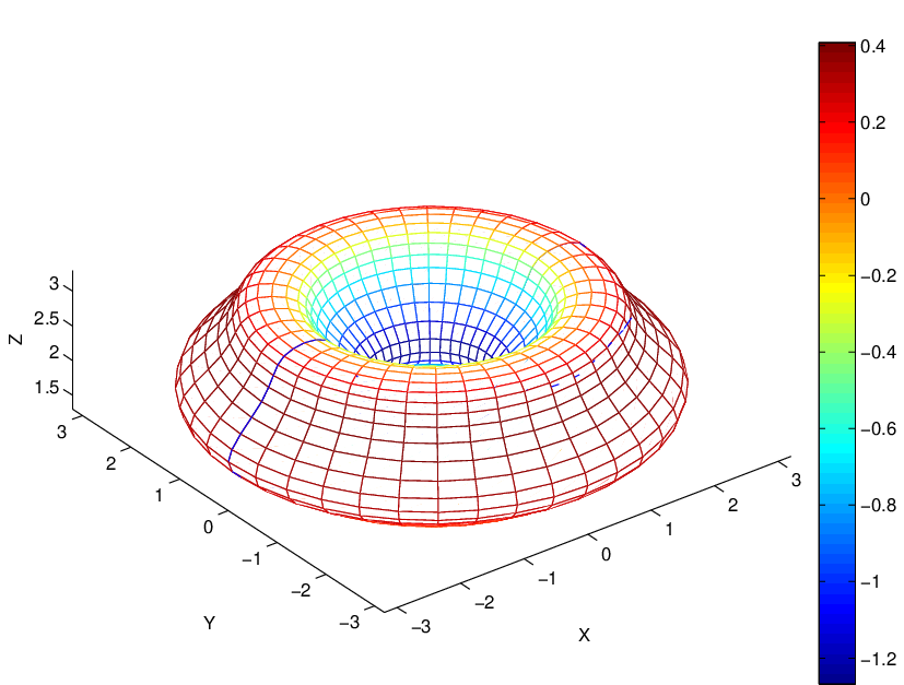
where the generating curve is smooth, with and (Fig. 1). It is straightforward to verify that
form a basis for the harmonic 1-forms on the surface .

In this setting, we may expand each scalar Debye source and , for , as a Fourier series in the direction:
Using this representation for the scalar sources leads to our electric and magnetic current-like variables via equations (41) and (42):
| (132) |
where and are globally defined orthonormal unit co-vectors defined along Recall from above that the harmonic 1-forms and ( and ) are constant in the azimuthal direction, so that they couple only to the purely axisymmetric () mode.
In short, the linear system (91), (99), (103) can be solved for each azimuthal mode separately. For nonzero azimuthal modes, where the harmonic 1-forms play no role, only equations (91), (99) are needed to determine for . For each mode the set of equations corresponds to a Fredholm system of equations of the second kind along the generating curve.
In a companion paper [5], we have developed a high-order accurate solver for scattering from closed surfaces of revolution, with a detailed description of the full algorithm. Here, we simply note that the method of [5] assumes an equi-spaced discretization of , and uses a pseudospectral approach for applying (or inverting) the surface Laplacian, the surface gradient, and the surface divergence. That is to say, differentiation is carried out in the transform domain, while multiplication by a variable coefficient function is carried out pointwise along . The principal value and weakly singular integrals which appear are computed using generalized Gaussian quadrature rules [1] with eighth or sixteenth order accuracy.
One issue that requires some care is the mean zero condition on the scalar sources. We showed, above, that the integral equation is invertible as a map from mean zero functions to mean zero functions. This condition is automatically satisfied for non-zero azimuthal modes (which necessarily integrate to zero). For the zero mode, one can either solve the integral equation iteratively, relying on the fact that the operator projects onto mean zero functions or add a rank-one modification to the system matrix to enforce invertibility of the discretized system and solve it directly. We have chosen the latter approach, described in more detail in [5].
Remark 3.
In the case of a perfect conductor, there are only two scalar source functions , expanded as above, with the electric and magnetic current-like variables computed from (18) and the condition .
Remark 4.
In the dielectric case, we still need to specify the choice of a clutching map. Our analysis above showed that a sufficient condition for uniqueness that avoids low frequency breakdown is to set on . Fig. 2 displays the condition number of the linear system for various choices of and .
Remark 5.
The second kind Fredholm system derived earlier for scattering from a dielectric is free from low frequency breakdown, as well as spurious resonances. An illustration of this is contained in Fig. 3, which shows the relative error in the electric and magnetic fields for the mode in the exterior and interior of the object in Fig. 1. The surface was discretized at 200 points in the direction using a sixteenth order hybrid Gauss-trapezoidal quadrature rule (see [1]). In order to calculate the accuracy of the scheme, two extra surfaces of revolution were constructed - one inside the scatterer and one outside. Smooth generalized Debye sources and harmonic vector fields were specified on each, and the electric and magnetic fields generated with the appropriate material parameters were evaluated on the surface of the scatterer. The source surface inside the scatterer gives rise to a field which is valid in the exterior of the scatterer, and the source surface outside the scatterer gives rise to a field which is valid in the interior of the scatterer. The tangential and normal components of the difference of these fields were taken as the boundary data. Using this boundary data, the generalized Debye sources and harmonic vector fields on the scatterer were calculated using the integral equation formulation for the dielectric. Lastly, the scattered field was evaluated and compared with the known fields generated by the two source surfaces.
Note that the error becomes even smaller at very small frequencies - this is because discretization errors that are introduced in the integral equation in terms that are and are suppressed as . Only the accuracy for the mode is plotted. The relative error, as a function of the frequency in the mode is indicative of that in a fully reconstructed scattering problem (i.e., after reassembling the orthogonal, azimuthally decoupled, field components).


7 Summary
We have developed a new integral representation for the solution of the time harmonic Maxwell equations in media with piecewise constant dielectric permittivity and magnetic permeability in In the simply connected case, we rely on four scalar densities (charge-like variables) rather than surface vector fields as our unknowns, and obtain a system of Fredholm equation of the second kind. In the multiply connected case, we supplement these unknowns with a basis for the surface harmonic 1-forms. The principal advantage of our approach is that it avoids the low frequency breakdown inherent in the classical method, due to Müller. Some subtlety arises in the selection of the interior and exterior representations. In Müller’s equation, the currents used to represent the interior and exterior fields are chosen to be scalar multiples of each other. In our case, we use a Hodge decomposition of the 1-forms and have introduced the clutching map in Section 3 to relate interior and exterior variables. We show that for stability in the zero frequency limit, the clutching map should act differently on the harmonic 1-forms and on their orthogonal complement.
A disadvantage of our approach is that we must construct current-like surface 1-forms through a non-local operator. In the present paper, we do this by inverting the Laplace-Beltrami operator, but other (spectrally equivalent) procedures can be applied that do not require the solution of a linear system of equations [3, 5].
References
- [1] B. K. Alpert, Hybrid Gauss-trapezoidal quadrature rules, SIAM J. Sci. Comput., 20 (1999), pp. 1551–1584.
- [2] D. Colton and R. Kress, Integral Equation Methods in Scattering Theory, Krieger Publishing Co., Malabar, Florida, reprint ed., 1992.
- [3] C. L. Epstein, Z. Gimbutas, L. Greengard, and A. Klöckner, A fast, stable integral equation method for electromagnetic scattering, in preparation, (2011).
- [4] C. L. Epstein and L. Greengard, Debye sources and the numerical solution of the time harmonic Maxwell equations, CPAM, 63 (2010), pp. 413–463.
- [5] C. L. Epstein, M. O’Neil, and L. Greengard, Stable, high-order methods for electromagnetic scattering from surfaces of revolution, in preparation, (2011).
- [6] J. D. Jackson, Classical Electrodynamics, 3rd ed., John Wiley and Sons, Hoboken, NJ, 1998.
- [7] C. Müller, Foundations of the Mathematical Theory of Electromagnetic Waves, vol. 155 of Die Grundlehren der mathematischen Wissenschaften in Einzeldarstellungen, Springer-Verlag, Berlin, Heidelberg, 1969.
- [8] J.-C. Nédélec, Acoustic and Electromagnetic Equations, vol. 144 of Applied Mathematical Sciences, Springer, New York, 2001.
- [9] C. H. Papas, Theory of Electromagnetic Wave Propagation, Dover, New York, 1988.
Appendix A The Boundary Operators
We now describe the limits of the tangential components of and along Along we can introduce an adapted local basis of orthonormal 1-forms, and the outward unit normal vector. In this basis we have The tangential part of at is the 1-form restricted to directions tangent to i.e., In terms of components along we identify the tangential part with
| (133) |
If the 2-form, then the tangential components of along are identified with the tangential components of the one-form wedged with
| (134) |
The normal component of is and that of is simply
The various boundary operators are given by:
is an operator of order and is an operator of order
These are operators of order
is an operator of order and is an operator of order