The small-maturity smile for exponential Lévy models

José E. Figueroa-López ^†^†thanks: Department of Statistics, Purdue University, W. Lafayette, IN, USA (figueroa@purdue.edu), work partially supported by the NSF grant # DMS 0906919. Martin Forde ^†^†thanks: Department of Mathematics, KingÕs College London, Strand, London WC2R 2LS (Martin.Forde@kcl.ac.uk).

Abstract

We derive a small-time expansion for out-of-the-money call options under an exponential Lévy model, using the small-time expansion for the distribution function given in Figueroa-López&Houdré[FLH09], combined with a change of numéraire via the Esscher transform. In particular, we find that the effect of a non-zero volatility $\sigma$ of the Gaussian component of the driving Lévy process is to increase the call price by $\frac{1}{2}\sigma^{2}t^{2}e^{k}\nu(k)(1+o(1))$ as $t\to 0$ , where $\nu$ is the Lévy density. Using the small-time expansion for call options, we then derive a small-time expansion for the implied volatility $\hat{\sigma}_{t}^{2}(k)$ at log-moneyness $k$ , which sharpens the first order estimate $\hat{\sigma}_{t}^{2}(k)\sim\frac{\frac{1}{2}k^{2}}{t\log(1/t)}$ given in [Tnkv10]. Our numerical results show that the second order approximation can significantly outperform the first order approximation. Our results are also extended to a class of time-changed Lévy models. We also consider a small-time, small log-moneyness regime for the CGMY model, and apply this approach to the small-time pricing of at-the-money call options; we show that for $Y\in(1,2)$ , $\lim_{t\to{}0}t^{-1/Y}\mathbb{E}(S_{t}-S_{0})_{+}=S_{0}\mathbb{E}^{*}(Z_{+})$ and the corresponding at-the-money implied volatility $\hat{\sigma}_{t}(0)$ satisfies $\lim_{t\to 0}\hat{\sigma}_{t}(0)/t^{1/Y-1/2}=\sqrt{2\pi}\,\mathbb{E}^{*}(Z_{+})$ , where $Z$ is a symmetric $Y$ -stable random variable under $\mathbb{P}^{*}$ and $Y$ is the usual parameter for the CGMY model appearing in the Lévy density $\nu(x)=Cx^{-1-Y}e^{-Mx}{\bf 1}_{\{x>0\}}+C|x|^{-1-Y}e^{-G|x|}{\bf 1}_{\{x<0\}}$ of the process.

1 Introduction

Lévy processes have played an important role in the development of financial models which can accurately approximate the so-called stylized features of historical asset prices and option prices. In the “statistical world”, financial asset prices exhibit distributions with heavy tails and high kurtosis as well as other dynamical features such as volatility clustering and leverage. In the “risk-neutral world”, market prices of vanilla options exhibit “skewed” implied volatilities (relative to changes in the strike), contradicting the classical Black-Scholes model which predicts a flat implied volatility smile. The smile phenomenon has been more pronounced after the 1987 market crash. Concretely, out-of-the-money equity put options typically bear a higher risk-premium (larger implied volatilities) than in-the-money puts. This effect is more dramatic as the time-to-maturity decreases. As explained in [CT04] (see Section 1.2.2), the latter empirical fact is viewed by many as a clear indication that a jump risk is recognized by the participants in the option market, and stochastic volatility models are, in general, not able to reproduce the pronounced implied volatility skew of short-term option prices unless the “volatility of volatility” is forced to take high values.

The literature on small-time asymptotics for option prices and implied volatilities has grown significantly during the last decade. For recent accounts of the subject in the case of stochastic volatility models, we refer the reader to [GHLOW09] for local volatility models, [FJL10] for the Heston model, [Forde09] for a general uncorrelated local-stochastic volatility model and [Forde10] for SABR type models. We concentrate here on asset price models with jumps. For an Itô semimartingale model for the underlying price process $(S_{t})$ , Carr&Wu[CW03] argued, by partially heuristic arguments, that the price of an out-of-the-money call option converges to zero at sharply different speeds depending on whether the underlying asset price process is purely continuous, purely discontinuous, or a combination of both. For instance, in the presence of jumps, they argue that the

\mathbb{E}(S_{t}-K)^{+}-(S_{0}-K)_{+}\sim c\,t,

(1)

for some constant $c\neq{}0$ , as the time-to-maturity $t$ tends to $0$ ¹¹ 1 Actually, [CW03] wrote $\Pi_{t}(K)-(S_{0}-K)_{+}=O(t)$ , even though in their empirical analysis they are assuming a stronger statement such as (1)., while the call price converges at the rate $O(e^{-c/t})$ for a purely-continuous model. These statements were subsequently exploited in [CW03] to investigate which kind of model is more adequate to describe the observed market option prices near to expiration. They concluded the necessity of both a continuous and a jump component to describe the implied volatility of S&P 500 index options and argued, based on simulation experiments, that the theoretical asymptotic behavior is usually manifested by options maturing within 20 days. We also refer the reader to [AS02] for further empirical evidence on the presence of both a continuous and jump component.

Using the closed-form expressions for call option prices, Boyarchenko&Levendorksii[BL02] (see also [Lev04a], [Lev04b], [Lev04c]) establish the following small-time asymptotic behaviour

\frac{1}{S_{0}}\mathbb{E}(S_{t}-K)_{+}\,\sim\,t{\int(e^{x}-e^{k})_{+}\nu(dx)},\quad\quad\quad\quad({k>0\quad\&\quad t\to 0})\,,

(2)

for several popular exponential Lévy models $S_{t}=S_{0}e^{X_{t}}$ , where $k$ is the log-moneyness $k:=\log(K/S_{0})$ and $\nu$ is the Lévy measure of the underlying Lévy process $(X_{t})$ . Subsequently, Levendorskii [Lev08] obtained (2) under certain technical conditions (see Theorem 2.1 therein), namely that $\int(|x|^{2}\wedge 1)e^{x+\varepsilon|x|}\nu(dx)<\infty$ for some $\varepsilon>0$ , and $\lim_{t\to{}0}\mathbb{E}(S_{t}-K)_{+}/t$ exists in the “out-of-the-money region”. More recently, Roper[Rop10] and Tankov [Tnkv10] prove that (2) holds for a general Lévy process $(X_{t})$ under mild conditions, using the first-order small-time moment asymptotic result

\lim_{t\to{}0}\frac{1}{t}\mathbb{E}\left\{\varphi(X_{t})\right\}=\int\varphi(x)\nu(dx),

(3)

valid for functions $\varphi$ that converges to $0$ as $x\to{}0$ at an appropriate rate (see, e.g. Figueroa-López[FL08] for details). In particular, it suffices that $\int_{|x|\geq 1}e^{x}\nu(dx)<\infty$ . [Lev08] also provides a natural generalization of (2) for a wide class of multi-factor Lévy and Markov models.

As a corollary of (2), [Rop10] and [Tnkv10] prove independently that the implied volatility $\hat{\sigma}_{t}(k)$ for exponential Lévy models explodes near expiration for out-of-the-money vanilla options. This is a very peculiar feature of financial models with jumps (see Remark 2.6 below for a brief discussion about its meaning). [Tnkv10] goes one step further and shows that

\hat{\sigma}_{t}^{2}(k)\sim\frac{\frac{1}{2}k^{2}}{t\log(1/t)}

(4)

as $t\to{}0$ . For at-the-money call option prices, [Rop10] also shows that the leading order term is $O(\sqrt{t})$ and does not depend on the jump component of the model. Moreover, the at-the-money implied volatility converges to the volatility of the Gaussian component of the driving Lévy process, and the limit is zero if the Lévy process has no Gaussian part. For bounded variation Lévy processes and for certain tempered-stable like Lévy processes, [Tnkv10] gives also the first-order asymptotic behavior of at-the-money implied volatilities. The asymptotic behavior (4) is in sharp contrast with a pure-continuous stochastic volatility model, where the implied volatility converges to a non-negative constant which depends on the shortest distance from zero to the vertical line with $x$ -coordinate equal to the log-moneyness of the call option, under the Riemmanian metric induced by the diffusion coefficient for the model (see, e.g. [GHLOW09], [FJL10], [Forde09], [Forde10]).

In this article, we extend previous results by computing the second order correction term $a_{1}(k)$ in the call option price approximation:

\frac{1}{t}\,\frac{1}{S_{0}}\mathbb{E}(S_{t}-K)_{+}\,=\,a_{0}(k)\,+\,a_{1}(k)\,t+o(t)\quad\quad\quad\quad(t\to 0)\,.

(5)

An important component in our proofs is played by the recent higher order small-time expansions for the distribution function of a Lévy process obtained in Figueroa-López&Houdré[FLH09]. In the spirit of the Black-Scholes formula and the classical change of numéraire, our approach exploits an appealing representation of the prices of out-of-the money options in terms of the tail distribution functions of the underlying Lévy process under both the original risk-neutral probability measure $\mathbb{P}$ and under the martingale probability measure $\mathbb{P}^{*}$ obtained when we take the stock as the numéraire; i.e. $\mathbb{P}^{*}(A):=\mathbb{E}\left(S_{t}1_{A}\right)$ (see e.g. Chapter 26 in [Bjr09] and references therein). The latter measure $\mathbb{P}^{*}$ is sometimes called Share measure (see e.g Carr&Madan[CM09]). Our results allow us to quantify precisely the effects of a non-zero Gaussian-component in the call option prices near expiration. We find that a continuous-component volatility of $\sigma$ will result in an call price increase of $\frac{1}{2}\sigma^{2}t^{2}e^{k}\nu(k)$ (per each dollar of the underlying spot price), where $\nu$ is the Lévy density and $k$ is the log-moneyness.

We also derive the corresponding small-time asymptotic behaviour for implied volatility, showing precisely how the implied volatility diverges to $\infty$ (see Section 2). We find that the dimensionless implied variance does tend to zero as we would expect, but very slowly; in fact slower than $t^{p}$ for any $p>0$ , and consequently the implied volatility explodes in the small-time limit. Furthermore, we characterize the asymptotic behavior of the relative error of the first order approximation, which is then used to obtain a second-order approximation for the implied volatility of out-of-the money call options. According to our numerical results (see Section 6 for the details), the second order approximation significantly reduces the error compared to that of the first order approximation, achieving up to a two-fold relative error reduction in some cases.

We later extend our analysis to the case of a time-changed exponential Lévy model $Z_{t}=X_{T_{t}}$ with an independent absolutely-continuous time change $T_{t}=\int_{0}^{t}Y_{s}ds$ satisfying some mild moment conditions (see Section 3). The time-changed Lévy model was proposed in [CGMY03] to incorporate the volatility clustering and leverage effects commonly exhibited by financial price processes. We show that the small-time behavior of call option prices depends not only on the triplet of the underlying Lévy process $X$ but also on the time-zero first and second moments of the speed process $(Y_{t})$ and the quantity

\gamma:=\lim_{t\searrow{}0}\frac{1}{t}\left[\mathbb{E}Y_{t}-\mathbb{E}Y_{0}\right],

which is assumed to exist. In some sense, $\gamma$ measures the current average acceleration of the random clock. Under mild conditions, we show that

\frac{1}{t}\,\frac{1}{S_{0}}\mathbb{E}(S_{t}-K)_{+}\,=\,\mathbb{E}Y_{0}a_{0}(k)\,+\,\big[\mathbb{E}Y_{0}^{2}a_{1}(k)+\gamma a_{0}(k)\big]\,t+o(t),\quad\quad\quad\quad(t\to 0)\,,

where $a_{0},a_{1}$ are the first and second order terms appearing in the pure-Lévy option price approximation (5). For a Cox-Ingersoll-Ross (CIR) speed process

dY_{t}=\kappa(\theta-Y_{t})dt+\sigma\sqrt{Y_{t}}dW_{t},\quad Y_{0}=y_{0}

the current acceleration of the process is $\gamma=\kappa(\theta-y_{0})$ and, hence, call option prices will exhibit the following small-maturity asymptotic behavior:

\frac{1}{t}\,\frac{1}{S_{0}}\mathbb{E}(S_{t}-K)_{+}\,=\,y_{0}a_{0}(k)\,+\,\big[y_{0}^{2}a_{1}(k)+\kappa(\theta-y_{0})a_{0}(k)\big]\,t+o(t),\quad\quad\quad\quad(t\to 0)\,.

As seen from this expression, a mean reversion speed of $\kappa$ will increase (resp., decrease) the call option price when the current volatility $y_{0}$ is above (resp. below) the long-run mean volatility value $\theta$ .

In Section 4, we also consider a small-time, small log-moneyness regime for the CGMY model of [CGMY02]. The CGMY model is a particular case of the more general KoBoL class of models, named after the authors [Kop95] (who first introduced the symmetric version of the model under the name of “truncated Lévy flights”) and [BL02]. Using the fact that $\left(X_{t}/t^{1/Y}\right)_{t}$ converges weakly to a symmetric alpha-stable distribution with $\alpha=Y$ as $t\to 0$ , we show that

\lim_{t\to{}0}t^{-1/Y}\frac{1}{S_{0}}\mathbb{E}(S_{t}-S_{0})_{+}=\mathbb{E}^{*}(Z_{+}),

for $Y\in(1,2)$ , where $Z$ is a symmetric $Y$ -stable random variable under $\mathbb{P}^{*}$ . We then apply this result to small-time pricing of at-the-money call options for the CGMY model. Our method of proof is new and based on the following representation by Carr&Madan[CM09]

\frac{1}{S_{0}}\mathbb{E}(S_{t}-K)_{+}=\mathbb{P}^{*}(X_{t}-E>\log\frac{K}{S_{0}})\,,

(6)

where $E$ is an independent exponential random variable under $\mathbb{P}^{*}$ with parameter 1. As a corollary, we conclude that the corresponding at-the-money implied volatility $\hat{\sigma}_{t}(0)$ satisfies $\lim_{t\to 0}\hat{\sigma}_{t}(0)/t^{1/Y-\frac{1}{2}}=\sqrt{2\pi}\,\mathbb{E}^{*}(Z_{+})$ . [Tnkv10] obtains a similar result in a more general model using a different approach based on a Fourier-type representation for call option prices. Let us also remark that the method of proof introduced here can be applied to a large class of Lévy processes whose Lévy densities are symmetric and dominated by stable Lévy densities, and behave like a symmetric $Y$ -stable process in the small-time limit (see Remark 4.3 for the details).

In section 5, we derive a similar small-time estimate for variance call options using the well known fact that the quadratic variation $[X]_{t}$ of a Lévy process is itself a Lévy process. Using the main result in [FL08], we find that an out-of-the-money variance call option which pays $([X]_{t}-K)_{+}$ at time $t$ is worth the same as a European-style contract paying $(\ln\frac{S_{t}}{S_{0}})^{2}-K)_{+}$ at time $t$ as $t\to 0$ , irrespective of the Lévy measure $\nu(\cdot)$ . The diffusion component of $(X_{t})$ does not show up at leading order for small $t$ . See also [KRMK11] for a related discussion on the difference between the small-time behaviour of variance call options on the exact quadratic variation and its discretely sampled approximation for Lévy driven models.

2 Small-time asymptotics for exponential Lévy models

Consider an exponential Lévy model for a stock price process

S_{t}=S_{0}e^{X_{t}}

(7)

where $(X_{t})$ is a Lévy process defined on a complete probability space $(\Omega,\mathbb{P},\mathcal{F})$ with generating triplet $(\sigma^{2},b,\nu)$ . We are assuming zero interest rate and dividend yield for simplicity ²² 2 For a non-zero constant interest rate $r$ and dividend rate $q$ , the results in this paper will not be qualitatively any different, because we can just replace the stock price process $(S_{t})$ with the forward price process $(e^{-(r-q)t}S_{t})_{t}$ , which is a martingale (see, e.g. Chapter 11 in [CT04]). and that $\mathbb{P}$ represents a risk-neutral pricing measure. We assume that $\int_{|x|>1}e^{x}\nu(dx)<\infty$ and that the following condition is satisfied

b+\frac{1}{2}\sigma^{2}+\int_{-\infty}^{\infty}(e^{x}-1-x1_{|x|\leq 1})\nu(dx)=0,

(8)

so that $S_{t}=S_{0}e^{X_{t}}$ is indeed a $\mathbb{P}$ -martingale relative to its own filtration.

Throughout the paper, we also assume that the Lévy measure $\nu(dx)$ admits a positive density, denoted $\nu(x)$ , and that this density is $C^{1}$ in $\mathbb{R}\backslash\{0\}$ satisfying $\sup_{|x|>\varepsilon}\nu(x)<\infty$ for every $\varepsilon>0$ . The choice between the Lévy measure $\nu(dx)$ and density $\nu(x)$ should be clear from the context. Under the previous standing condition, Figueroa-López&Houdré [FLH09] show the following result (see Remark 3.3 and Proposition 3.4 therein):

Theorem 2.1

[FLH09]. Let $y>0$ be fixed. Then, we have the following small-time behaviour for the distribution function of $X_{t}$ :

\frac{1}{t}\,\mathbb{P}(X_{t}\geq y)=\nu[y,\infty)+\frac{1}{2}t{d_{2}(y)}+o(t)\quad\quad\quad\quad(t\to 0)\,,

where

	$\displaystyle d_{2}(y)$	$\displaystyle=$	$\displaystyle d_{2}(y;b,\sigma,{\nu})=-\sigma^{2}\nu^{\prime}(y)+2b\nu(y)-\nu[y,\infty)^{2}+\nu(\frac{1}{2}y,y)^{2}$		(9)
		$\displaystyle+$	$\displaystyle 2\int_{-\infty}^{-\frac{1}{2}y}\int_{y-x}^{y}\nu(u)\nu(x)dudx-2\nu(y)\int_{\frac{1}{2}y<\|x\|<1}x\nu(x)dx+2\nu(y)\int_{-\frac{1}{2}y}^{\frac{1}{2}y}\int_{y-x}^{y}(\nu(u)-\nu(y))\nu(x)dudx\,.$		(9)

Furthermore, if the pure-jump component of $(X_{t})$ has finite variation, i.e. $\int_{|x|\leq 1}|x|\nu(dx)<\infty$ , then $d_{2}$ simplifies to

d_{2}(y)=d_{2}(y;b,\sigma,\nu)=-\sigma^{2}\nu^{\prime}(y)+2b_{0}\nu(y)-\nu[y,\infty)^{2}+\int_{0}^{y}\int_{y-x}^{y}\nu(u)\nu(x)dudx-2\int_{y}^{\infty}\int_{-\infty}^{y-x}\nu(u)\nu(x)dudx\,,

(10)

where $b_{0}$ is the drift of the pure-jump component of $(X_{t})$ defined by $b_{0}=b-\int_{|x|\leq 1}x\nu(dx)$ .

Remark 2.1

The double integrals in (9) and (10) are well-defined. For instance, by the symmetry of $s(u)s(x)$ about the line $u=x$ ,

$\displaystyle\int_{0}^{y}\int_{y-x}^{y}\nu(u)\nu(x)dudx$	$\displaystyle=\int_{0}^{y/2}\int_{y-x}^{y}\nu(u)\nu(x)dudx+\int_{y/2}^{y}\int_{y-x}^{y/2}\nu(u)\nu(x)dudx+\int_{y/2}^{y}\int_{y/2}^{y}\nu(u)\nu(x)dudx$
	$\displaystyle=2\int_{0}^{y/2}\int_{y-x}^{y}\nu(u)\nu(x)dudx+\int_{y/2}^{y}\int_{y/2}^{y}\nu(u)\nu(x)dudx$	(11)
	$\displaystyle\leq 2[\sup_{u\in(y/2,y)}\nu(u)]\int_{0}^{y/2}x\nu(x)dx+[(y/2)\sup_{u\in(y/2,y)}\nu(u)]^{2},$

which is finite because $\int_{|x|\leq{}1}|x|\nu(x)dx<\infty$ (being $X$ a bounded variation process). To obtain the bound on the first integral (11), we used the fact that the range for $x$ is from $0$ to $y/2$ and, hence, the maximal range for u in the inner integral is $u\in[y/2,y]$ . Similarly, by Fubini’s theorem,

	$\displaystyle\int_{y}^{\infty}\int_{-\infty}^{y-x}\nu(u)\nu(x)dudx$	$\displaystyle=\int_{-\infty}^{0}\int_{y}^{y-u}\nu(u)\nu(x)dxdu$
		$\displaystyle\leq\int_{-1}^{0}\int_{y}^{y-u}\nu(x)dx\nu(u)du+\int_{-\infty}^{-1}\int_{y}^{y-u}\nu(x)dx\nu(u)du$
		$\displaystyle\leq[\sup_{x>y}\nu(x)]\int_{-1}^{0}(-u)\nu(u)du+\int_{-\infty}^{-1}\nu(u)du\int_{y}^{\infty}\nu(x)dx<\infty.$

In the following proposition, we use Theorem 2.1 to establish a small-time estimate for the price of an out-of-the-money call option under the model in (7):

Proposition 2.2

Assume that

(i)\;\int_{|x|>1}e^{x}\nu(x)dx<\infty\,\quad\text{and}\quad(ii)\;\sup_{|x|>\varepsilon}e^{x}\nu(x)<\infty,

(12)

for any $\varepsilon>0$ . Then we have the following small-time expansion for the price of a call option with strike $K>S_{0}$

\frac{1}{t}\,\mathbb{E}(S_{t}-K)_{+}\,=\,S_{0}\int_{-\infty}^{\infty}(e^{x}-e^{k})_{+}\nu(x)dx\,+\,\frac{1}{2}S_{0}\big[d_{2}^{*}(k)-e^{k}d_{2}(k)\big]t+o(t)\quad\quad\quad\quad(t\to 0)\,,

(13)

where $k=\log\frac{K}{S_{0}}>0$ is the log-moneyness and $d_{2}^{*}(k)=d_{2}(k;b^{*},\sigma,\nu^{*})$ with $b^{*}$ and ${\nu^{*}}$ given by

{\nu^{*}(x)=e^{x}\nu(x)}\quad\text{and}\quad b^{*}=b+\int_{|x|\leq{}1}x\left(e^{x}-1\right)\nu(x)dx+\sigma^{2}.

(14)

Remark 2.2

This result sharpens the asymptotic behavior (2), established by Levendorskii [Lev08] for a class of multi-factor Lévy and Markov models under certain technical conditions. As explained in the introduction, for a Lévy model, these conditions were relaxed by Roper[Rop10] and Tankov [Tnkv10]. Note also that, by imposing that $\nu$ has a positive Lévy density, we are precluding the Black-Scholes case where there is a non-zero diffusion component with volatility $\sigma$ and zero jump component, for which the implied volatility is just constant and equal to $\sigma$ .

Proof.

Without loss of generality, we assume that $(X_{t})$ is the canonical process $X_{t}(\omega)=\omega(t)$ defined on $\Omega=\mathbb{D}([0,\infty),\mathbb{R})$ (the space of right-continuous functions with left limit $\omega:[0,\infty)\to\mathbb{R}$ ) and equipped with the $\sigma-$ field $\mathcal{F}=\sigma(X_{s}:s\geq{}0)$ and the right-continuous filtration $\mathcal{F}_{t}:=\cap_{s>t}\sigma(X_{u}:u\leq{}s)$ . Following the density transformation construction of Sato[Sat99] (see Definition 33.4 and Example 33.4 therein) and using the martingale condition (8), we define $\mathbb{P}^{*}$ on $(\Omega,\mathcal{F})$ such that

\mathbb{P}^{*}(B)=\mathbb{E}\left(e^{X_{t}}1_{B}\right),

(15)

for any $t>0$ and $B\in\mathcal{F}_{t}$ . As explained in the introduction, we can interpret $\mathbb{P^{*}}$ as the martingale measure associated with using the stock price as the numéraire.

Let us first note that the price of a call option can be decomposed as follows:

$\displaystyle\mathbb{E}(S_{t}-K)_{+}$	$\displaystyle=$	$\displaystyle\mathbb{E}(S_{t}1_{S_{t}\geq K})-K\mathbb{P}(S_{t}\geq K)$	(16)
	$\displaystyle=$	$\displaystyle S_{0}\mathbb{E}(e^{X_{t}}1_{S_{t}\geq K})-S_{0}e^{k}\mathbb{P}(X_{t}\geq k)$
	$\displaystyle=$	$\displaystyle S_{0}\mathbb{P}^{*}(X_{t}\geq k)-S_{0}e^{k}\mathbb{P}(X_{t}\geq k)$

One can check that $(X_{t})$ is a Lévy process under $\mathbb{P}^{*}$ with characteristic triplet $(b^{*},\sigma^{2},\nu^{*})$ . For this result see the more general Theorem 33.1 in Sato[Sat99]. Finally, applying Theorem 2.1 to the probabilities under $\mathbb{P}$ and $\mathbb{P}^{*}$ in (16), we have

{\frac{1}{t}\,\mathbb{E}(S_{t}-K)_{+}\,=\,S_{0}\int_{k}^{\infty}e^{x}\nu(x)dx-K\int_{k}^{\infty}\nu(x)dx\,+\,\frac{1}{2}S_{0}d_{2}^{*}(k)t-\frac{1}{2}Kd_{2}(k)t+o(t)\quad\quad\quad\quad(t\to 0)\,,}

(17)

which simplifies to (13). ∎

Remark 2.3

Let us note that for a bounded variation process, the drift of $X$ under the Share measure $\mathbb{P}^{*}$ is the same as the drift under the measure $\mathbb{P}$ . Indeed, denoting $b^{*}_{0}$ the drift under $\mathbb{P}^{*}$ , we have that

b^{*}_{0}=b^{*}-\int_{\{|x|\leq{}1\}}x\nu^{*}(x)dx=b+\int_{|x|\leq{}1}x\left(e^{x}-1\right)\nu(x)dx-\int_{\{|x|\leq{}1\}}xe^{x}\nu(x)dx=b_{0}.

Also, note that the call price approximation (13) is independent of $b$ . Indeed, let

R(y;\nu):=d_{2}(k;b,\sigma,\nu)-\left(-\sigma^{2}\nu^{\prime}(y)+2b\nu(y)\right),

which depends only on $\nu$ as seen from the expression of $d_{2}$ in (9). Then, using (14), the second order term in (13) can be simplified as follows

	$\displaystyle a_{1}(k):=a_{1}(k;b,\sigma,\nu)$	$\displaystyle:=\frac{1}{2}\big[d_{2}(k;b^{},\sigma,\nu^{})-e^{k}d_{2}(k;b,\sigma,\nu)\big]$
		$\displaystyle=\frac{\sigma^{2}}{2}e^{k}\nu(k)+e^{k}\nu(k)\int_{\|x\|\leq{}1}x\left(e^{x}-1\right)\nu(x)dx+\frac{1}{2}\left[R(k;\nu^{*})-e^{k}R(k;\nu)\right],$

which does not depend on $b$ . The previous expression also shows that

a_{1}(k;b,\sigma,\nu)-a_{1}(k;b,0,\nu)=\frac{\sigma^{2}}{2}e^{k}\nu(k),

and, hence, a non-zero volatility of $\sigma$ has the effect of increasing the call price approximation by $\frac{\sigma^{2}t^{2}}{2}e^{k}\nu(k)$ .

2.1 Implied volatility

Let $\hat{\sigma}_{t}(k)$ denote the Black-Scholes implied volatility at log-moneyness $k$ and maturity $t$ with zero interest rates, and let $V(t,k)=\hat{\sigma}_{t}(k)^{2}t$ denote the dimensionless implied variance. Let

\displaystyle a_{0}(k):=\int_{-\infty}^{\infty}(e^{x}-e^{k})_{+}{\nu(dx)}\quad\text{and}\quad a_{1}(k):=\frac{1}{2}\big[d_{2}^{*}(k)-e^{k}d_{2}(k)\big]

(18)

denote the (normalized) leading order and correction terms in (13). By put-call parity, the dominated convergence theorem, and the stochastic continuity of the Lévy process $(X_{t})$ , we have

\lim_{t\to 0}\mathbb{E}(S_{t}-K)_{+}=(S_{0}-K)_{+}\,,

and from this we can show that $V(t,k)\to 0$ as $t\to 0$ . The following corollary shows more precisely how $V(t,k)\to 0$ as $t\to 0$ and, hence, sharpening a result in Tankov [Tnkv10] (Proposition 4 therein):

Theorem 2.3

For the exponential Lévy model in (7), we have the following small-time behavior for the implied variance $V(t,k)$ for $k>0$

V(t,k)=V_{0}(t,k)\big[1+V_{1}(t,k)\,+\,o(\frac{1}{\log\frac{1}{t}})\big]\quad\quad\quad\quad(t\to 0),

(19)

where

	$\displaystyle V_{0}(t,k)$	$\displaystyle=$	$\displaystyle\frac{\frac{1}{2}k^{2}}{\log(\frac{1}{t})}\,,$
	$\displaystyle V_{1}(t,k)$	$\displaystyle=$	$\displaystyle\frac{1}{\log(\frac{1}{t})}\log\left[\frac{4\sqrt{\pi}a_{0}(k)e^{-k/2}}{k}\left[\log\left(\frac{1}{t}\right)\right]^{3/2}\right]\,.$		(20)

Proof.

See Appendix A.∎

Remark 2.4

Multiplying (19) by $1/t$ , we have the following expansion for the implied volatility

\hat{\sigma}^{2}_{t}(k)=\frac{\frac{1}{2}k^{2}}{t\log(\frac{1}{t})}\big[1\,+\,V_{1}(t,k)\,+\,o(\frac{1}{\log\frac{1}{t}})]\,\quad\quad\quad\quad(t\to 0),

(21)

and we see that $\hat{\sigma}^{2}_{t}(k)\to\infty$ as $t\to{}0^{+}$ , as is well documented in e.g. Carr&Wu[CW03] (see also Roper[Rop10] and [Tnkv10]). The leading order term agrees with that obtained in Tankov[Tnkv10] and, moreover, we see that

[t\log(\frac{1}{t})]^{\frac{1}{2}}\hat{\sigma}_{t}(k)\sim|k|/\sqrt{2},\quad\quad\quad\quad(t\to 0)\,,

so the (re-scaled) leading order implied volatility smile is V-shaped and independent of $\nu$ , except that we require $\nu$ to be non-zero.

Remark 2.5

$V(t,k)=O(\frac{1}{\log\frac{1}{t}})$ , so $V(t,k)\to 0$ but slowly; in fact slower than $t^{p}$ for any $p>0$ . In particular, for a given desired “precision” bound $\varepsilon\ll 1$ , we will need $t=O(e^{-1/\epsilon})$ to ensure that $V(t,k)=O(\epsilon)$ and for the $\frac{1}{\log\frac{1}{t}}$ error term in (19) to be $O(\epsilon)$ . For this reason, the call option estimate (13) is more useful than the implied volatility estimate (21) in practice. We remark that in Corollary 8.3 of the very recent article by Gao&Lee[GL11], the authors give an expansion which sharpens (19), but proving their result is more involved and requires several preliminary lemmas

Remark 2.6

Based on high-frequency statistical methods for Itô semimartingales, several empirical studies have statistically rejected the null hypothesis of either a purely-jump or a purely-continuous model (see, e.g., [AJ09b], [AJ10], [BNS06]). If this really is the case, then our results show that theoretically, the small-maturity smile must tend to infinity, if put/call options are priced correctly. Nevertheless, this effect is often obscured in reality by market practicalities - high bid/offer spreads, daycount/settlement conventions, and times when the market is closed. However, even if we cannot trade an option with infinitesimally small maturity in practice, we can still look at rate at which the implied volatility smile steepens as the maturity goes small; typically it is difficult to fit the one of the fashionable class of purely continuous models (e.g. Heston, SABR, and other local-stochastic volatility hybrid models) to this kind of data, with realistic parameters. Carr&Wu[CW03]’s study of S&P 500 option price data (in contrast to the previous statistical approaches) also suggests that the sample path of the index contains both continuous and discontinuous martingale components (working under a risk neutral measure), and that, while the presence of the jump component varies strongly over time, the continuous component is omnipresent.
In the same vein, Aït-Sahalia&Jacod[AJ09a] define a jump activity index to test for the presence of jumps, which for a Lévy process coincides with the Blumenthal-Getoor index of the process. [AJ09a] also proposes estimators of this index for a discretely sampled process and derive the estimators’ properties. These estimators are applicable despite the presence of a Brownian component in the process, which makes it more challenging to infer the characteristics of the small, infinite activity jumps. When the method is applied to high frequency stock returns, [AJ09a] found evidence of infinitely active jumps in the data and they were able to estimate the index of activity.

3 Time-changed Lévy processes

3.1 A formula for out-of-the-money call option prices

In addition to the Lévy process $(X_{t})$ of Section 2, we now consider a random clock $(T_{t})$ defined on $(\Omega,\mathbb{P},\mathcal{F})$ and independent of $X$ . A random clock is a right-continuous non-decreasing process such that $T_{0}=0$ . We consider a time-changed Lévy model of the form

S_{t}:=S_{0}e^{Z_{t}},\quad{\text{with}\quad Z_{t}:=X_{T_{t}}}.

(22)

As explained in the introduction, this type of model is important because it can incorporate volatility clustering effects.

Given that $e^{X_{t}}$ is a martingale under $\mathbb{P}$ (relative to the natural filtration generated by $X$ ), it is known that $(S_{t})$ above is a martingale under $\mathbb{P}$ relative to the natural filtration generated by the random clock $T_{t}$ and the time-changed process $Z_{t}$ (see Lemma 15.2 in [CT04]). Note also that our simplifying assumption (8) implies that

S_{t}=S_{0}\frac{e^{Z_{t}}}{\mathbb{E}(e^{Z_{t}})}

(23)

because $\mathbb{E}(e^{Z_{t}})=1$ . [CGMY03] (Section 4.2) shows that the price process (23) is free of static arbitrage opportunities. Furthermore, under certain conditions (e.g. if $X$ has infinite jump activity and $(T_{t})$ is continuous), $\sigma(T_{u}:u\leq{}t)\subset\sigma(X_{T_{u}}:u\leq{}t)$ (see, e.g., Theorem 1 in [Win01]), and hence (22) will be a martingale relative to the filtration generated by only the time-changed process $(Z_{t})$ or, equivalently, the filtration generated by the stock-price process $(S_{t})$ . In that case, the model (22) will be free of dynamic arbitrage opportunities by the sufficiency part of the First Fundamental Theorem of Asset Pricing.

Let $\mathcal{N}$ be the set of $\mathbb{P}$ -null sets of $\mathcal{F}$ and define a probability measure $\widetilde{\mathbb{P}}$ on $\widetilde{\mathcal{F}}:=\sigma(Z_{t},T_{t}:t>{}0)\vee\mathcal{N}$ such that, for any $t>0$ ,

\widetilde{\mathbb{P}}(B)=\mathbb{E}\left(e^{Z_{t}}1_{B}\right),

(24)

whenever $B\in\widetilde{\mathcal{F}}_{t}:=\sigma(Z_{u},T_{u}:u\leq t)\vee\mathcal{N}$ . We note that $\widetilde{\mathbb{P}}$ is well defined since $\{e^{Z_{t}}\}_{t\geq{}0}$ is a $\mathbb{P}$ -martingale relative to $\{\widetilde{\mathcal{F}}_{t}\}_{t\geq{}0}$ . The following proposition will play a key role in the sequel:

Proposition 3.1

Suppose that the assumptions of Proposition 2.2 are satisfied and let $(b^{*},\sigma^{2},\nu^{*})$ be defined as in (14). Then, under $\widetilde{\mathbb{P}}$ , the process $\left(Z_{t}\right)$ in (22) has the same distribution as a Lévy process with the characteristic triplet $(b^{*},\sigma^{2},\nu^{*})$ evaluated at the independent random clock $T_{t}$ .

Proof.

Fix $0=t_{0}<\dots<t_{n}=t<\infty$ and $u_{1},\dots,u_{n}\in\mathbb{R}$ . Then, using the independence between $T$ and $X$ ,

	$\displaystyle\widetilde{\mathbb{E}}(\exp\{i\sum_{j=1}^{n}u_{j}(Z_{t_{j}}-Z_{t_{j-1}})\})$	$\displaystyle=\mathbb{E}(\exp\{Z_{t}+i\sum_{j=1}^{n}u_{j}(Z_{t_{j}}-Z_{t_{j-1}})\})=\mathbb{E}(\exp\{\sum_{j=1}^{n}i(u_{j}-i)(X_{T_{t_{j}}}-X_{T_{t_{j-1}}})\})$
		$\displaystyle=\mathbb{E}(\exp\{\sum_{j=1}^{n}(T_{t_{j}}-T_{t_{j-1}})\psi(u_{j}-i)\})=\mathbb{E}(\exp\{\sum_{j=1}^{n}(T_{t_{j}}-T_{t_{j-1}})\psi^{*}(u_{j})\})\,.$

The last expression corresponds to the characteristic function of a process of the form $X^{*}_{T_{t}}$ , where $(X^{*}_{t})$ is a Lévy process with triplet $(b^{*},\sigma^{2},\nu^{*})$ defined on $(\Omega,\mathbb{P},\mathcal{F})$ and independent of the random clock $(T_{t})$ . ∎

In light of the previous result, we have the following representation for call option prices:

$\displaystyle\mathbb{E}(S_{t}-K)_{+}$	$\displaystyle=$	$\displaystyle\mathbb{E}(S_{t}1_{S_{t}\geq K})-K\mathbb{P}(S_{t}\geq K)$	(25)
	$\displaystyle=$	$\displaystyle S_{0}\mathbb{E}(\exp(Z_{t})1_{Z_{t}\geq k})-S_{0}e^{k}\mathbb{P}(S_{t}\geq K).$
	$\displaystyle=$	$\displaystyle S_{0}\widetilde{\mathbb{P}}\left(Z_{t}\geq k\right)-S_{0}e^{k}\mathbb{P}(Z_{t}\geq k).$

We emphasize again that, under $\widetilde{\mathbb{P}}$ , $Z_{t}$ has the same distribution as a Lévy process with characteristic triplet $(b^{*},\sigma^{2},\nu^{*})$ evaluated at an independent random clock $(T_{t})$ . Hence, as for the pure-Lévy model case, the problem of finding small-time expansions for out-the-money option prices reduces to finding small-time asymptotics of the corresponding distribution functions.

3.2 Small-time asymptotics for the time-changed Lévy model

In this section, we determine the asymptotic behavior of out-the-money call option prices. We consider random clocks $(T_{t})$ that are absolutely continuous with non-negative rate process $(Y_{t})$ (i.e. $T_{t}=\int_{0}^{t}Y_{s}ds$ ) such that $Y_{0}>0$ . We will also refer to the following conditions in the sequel:

		$\displaystyle{\bf(i)}\;\;\mathbb{E}Y_{t}-\mathbb{E}Y_{0}=O(t),\quad{\bf(ii)}\;\;\limsup_{t\searrow{}0}\,\mathbb{E}Y^{2}_{t}<\infty,\quad{{\bf(iii)}\;\;\lim_{t\searrow{}0}\frac{1}{t}\left[\mathbb{E}Y_{t}-\mathbb{E}Y_{0}\right]=\gamma\in[0,\infty)},$		(26)
		$\displaystyle{\bf(iv)}\;\;\limsup_{t\searrow{}0}\,\mathbb{E}Y_{t}^{3}<\infty,\quad{\bf(v)}\;\;\lim_{t\searrow{}0}\frac{1}{t^{2}}\mathbb{E}T_{t}^{2}=\rho\in(0,\infty).$		(27)

In the case that $(Y_{t})$ is a stationary process with finite moment of third order, $\mathbb{E}Y_{t}^{k}$ is constant for $k=1,\dots,3$ and (i)-(iv) are automatically satisfied. Also, if $Y_{t}\to{}Y_{0}$ and (iv) are satisfied, then (v) holds true with $\rho=\mathbb{E}\,Y_{0}^{2}$ . Indeed, note first that $\lim_{s\to{}0}\mathbb{E}\,Y_{s}^{2}=\mathbb{E}\,Y_{0}^{2}$ since ${(Y_{t}^{2})_{t<t_{0}}}$ are uniformly integrable for small enough $t_{0}$ by (iv) above. Also, since ${T_{t}^{2}/t^{2}\leq\int_{0}^{t}Y_{s}^{2}ds/t}$ (by Jensen’s inequality) and $\lim_{t\to{}0}\mathbb{E}\int_{0}^{t}Y_{s}^{2}ds/t=\mathbb{E}\lim_{t\to{}0}\int_{0}^{t}Y_{s}^{2}ds/t$ , so the dominated convergence theorem implies that

\lim_{t\to{}0}\frac{1}{t^{2}}\mathbb{E}T_{t}^{2}=\mathbb{E}\lim_{t\to{}0}\left(\frac{1}{t}\int_{0}^{t}Y_{s}ds\right)^{2}=\mathbb{E}Y_{0}^{2}.

The following result gives the small-time asymptotic behavior of the tail distributions of time-changed Lévy models:

Theorem 3.2

Suppose that the conditions of Theorem 2.1 are satisfied as well as conditions (i)-(ii) of (26). Then,

\mathbb{P}(Z_{t}\geq{}x)=t\mathbb{E}Y_{0}\nu[x,\infty)\left[1+O(t)\right],\quad\quad\quad\quad(t\to 0).

(28)

If, additionally, conditions (iii)-(v) of (27) are satisfied, then

\mathbb{P}(Z_{t}\geq{}x)=t\mathbb{E}Y_{0}\nu[x,\infty)+{\frac{1}{2}\left(\rho\,d_{2}(x)+\gamma\nu[x,\infty)\right)}t^{2}+o(t^{2}),\quad\quad\quad\quad(t\to 0),

(29)

where $d_{2}$ is the same as in Theorem 2.1.

Proof.

See Appendix A.∎

Remark 3.1

A very popular rate process in applications is the Cox-Ingersoll-Ross (CIR) diffusion process, defined by

dY_{t}=\kappa(\theta-Y_{t})dt+\sigma\sqrt{Y_{t}}dW_{t},

(30)

where $(W_{t})$ is a standard Brownian motion, $Y_{0}$ is an integrable positive random variable independent of $W$ , and $\kappa,\theta,\sigma>0$ are such that $\kappa\theta/\sigma^{2}>1/2$ (which ensures that $Y=0$ is an inaccessible boundary). If $Y_{0}\sim\Gamma(\frac{2\theta\kappa}{\sigma^{2}},\frac{\sigma^{2}}{2\kappa})$ , the proces $(Y_{t})$ is stationary and $\mathbb{E}Y_{t}^{k}$ is finite and constant in $t$ for any $k\geq{}1$ . In particular, (i)-(v) are satisfied with $\rho=\mathbb{E}Y_{0}^{2}$ . In the non-stationary case, it is known that $\mathbb{E}Y_{t}-\mathbb{E}Y_{0}=\left(\theta-\mathbb{E}Y_{0}\right)\left(1-e^{-\kappa t}\right)$ and (i) & (iii) are satisfied with $\gamma={\kappa}(\theta-\mathbb{E}Y_{0})$ . The other conditions in (26-27) will also hold true. Thus we conclude that the time-changed Lévy model with CIR speed process satisfies:

\mathbb{P}(Z_{t}\geq{}x)=t\mathbb{E}Y_{0}\nu[x,\infty)+\left(\mathbb{E}Y_{0}^{2}\,d_{2}(x)+{\kappa}(\theta-\mathbb{E}Y_{0})\nu[x,\infty)\right)\frac{1}{2}t^{2}+o(t^{2}),\quad\quad\quad\quad(t\to 0).

We are now ready to give the small-time asymptotic behavior of out-the-money call option prices and the corresponding implied volatility:

Corollary 3.3

Under the conditions of Proposition 3.2, we have the following small-time expansions

\frac{1}{t}\,\mathbb{E}(S_{t}-K)_{+}\,=\,S_{0}\mathbb{E}Y_{0}a_{0}(k)\,+\,S_{0}{\big[\rho a_{1}(k)+\gamma a_{0}(k)\big]}t+o(t)\quad\quad\quad\quad(t\to 0)\,,

(31)

where $k=\log K/S_{0}>0$ and $a_{0},a_{1}$ are the first and second order terms of the call price approximation (13) as defined in (18). Furthermore, we have the following small-time behaviour for the implied variance $V(t,k)$ for $k>0$

V(t,k)=V_{0}(t,k)\big[1+V_{1}(t,k)\,+\,o(\frac{1}{\log\frac{1}{t}})\big]\quad\quad\quad\quad(t\to 0),

(32)

where

	$\displaystyle V_{0}(t,k)$	$\displaystyle=$	$\displaystyle\frac{\frac{1}{2}k^{2}}{\log(\frac{1}{t})}\,,$
	$\displaystyle V_{1}(t,k)$	$\displaystyle=$	$\displaystyle\frac{1}{\log(\frac{1}{t})}\log\left(\frac{4\sqrt{\pi}\,\mathbb{E}(Y_{0})a_{0}(k)e^{-k/2}}{k}\left[\log\left(\frac{1}{t}\right)\right]^{3/2}\right)\,.$		(33)

Proof.

The expansion (31) follows from the representation (25) and (29). The asymptotics (32) follows from the proof of Thorem 2.3. ∎

Remark 3.2

As it was indicated before, the time-changed Lévy model (22) was introduced to account for the volatility clustering exhibited by financial time series. Indeed, the process $(Y_{t})_{t}$ controls the speed of the random clock so that when $Y_{t}$ is high, the random clock runs faster and, hence, the price process exhibits more variability. Another approach to incorporate stochastic volatility is via stochastic integration along the lines of the following jump-diffusion model

d\ln(S_{t}/S_{0})=\mu(Y_{t})dt+\sigma(Y_{t})dW_{t}^{1}+dZ_{t},\quad dY_{t}=\alpha(Y_{t})dt+\gamma(Y_{t})dW_{t}^{(2)},

(34)

where $W^{(1)}$ and $W^{(2)}$ are two (possibly correlated) Brownian motions and $Z$ is a pure-jump process. For a comparison of these two methods, we refer the reader to Chapter 15 of [CT04]. Recently, [FLGH11] have provided small-time expansions for vanilla option prices under the stochastic model (34) when $Z$ is a pure-jump Lévy process independent of $Y$ .

4 Small-time, small log-moneyness asymptotics

In this section, we survey the behavior of $\mathbb{P}(X_{t}\geq k)$ for a Lévy process $X$ , when $t\to{}0$ and $k=k_{t}$ also converges to zero at an appropriate rate. We can think of this scaling as a small-time, small log-moneyness regime. As an application, we deduce the asymptotic behavior of at-the-money call option prices for a CGMY model.

4.1 Lévy models with non-zero Brownian component

Several financial models in the literature consist of a Lévy model with non-zero Brownian component. The most popular models of this kind are the Merton model and Kou model determined by the characteristic functions

	$\displaystyle\mathbb{E}(\exp(iuX_{t}))$	$\displaystyle=\exp[t(ibu-\frac{1}{2}\sigma^{2}u^{2}+iu\lambda\,(\frac{p}{\lambda_{+}-iu}-\frac{1-p}{\lambda_{-}+iu}))],$
	$\displaystyle\mathbb{E}(\exp(iuX_{t}))$	$\displaystyle=\exp[t(ibu-\frac{1}{2}\sigma^{2}u^{2}+\lambda\,(e^{-\delta^{2}u^{2}/2+i\mu u}-1))].$

It turns out that, for a general Lévy process $(X_{t})$ with $\sigma\neq{}0$ ,

\lim_{t\to 0}\mathbb{E}(\exp(iuX_{t}/\sqrt{t}))=\exp(-\frac{1}{2}\sigma^{2}u^{2})\,,

(see e.g. pp. 40 in [Sat99] for a formal proof). The right-hand side is the characteristic function of a Normal $N(0,\sigma^{2})$ random variable $Z$ , thus $(X_{t}/\sqrt{t})$ converges weakly to a Normal distribution with variance $\sigma^{2}$ and

\lim_{t\to 0}\mathbb{P}(X_{t}/\sqrt{t}>x)=\mathbb{P}(Z>x)\,.

4.2 The CGMY model and other tempered stable models

The so-called CGMY model is a pure-jump Lévy process determined by a Lévy density of the form

\displaystyle{\nu(x)=\frac{Ce^{-Mx}}{x^{1+Y}}\,{\bf 1}_{\{x>0\}}+\frac{Ce^{Gx}}{|x|^{1+Y}}\,{\bf 1}_{\{x<0\}}}.

(35)

for $C,G,M>0$ and $Y\in(0,2)$ . As explained in the introduction, the CGMY model is a particular case of the more general KoBoL class of models, named after the authors [Kop95] (who first introduced the symmetric version of the model under the name of “truncated Lévy flights”) and [BL02]. The term CGMY was introduced later on by Carr et al. [CGMY02]. This process is a tempered stable process (see Section 4.5 in Cont&Tankov[CT04]), and its characteristic function is given as

{\phi_{t}(u)=\mathbb{E}(e^{iuX_{t}})=\exp\left[t\,C\Gamma(-Y)\left\{(M-iu)^{Y}+(G+iu)^{Y}-M^{Y}-G^{Y}\right\}+i{\hat{b}}ut\right]},

(36)

for $Y\neq{}1$ and some constant $\hat{b}\in\mathbb{R}$ (see [CT04] for the formula when $Y=1$ ). We note that we must have $M>1$ for (12) to be satisfied, and under this condition, $X$ is again a CGMY process under $\mathbb{P}^{*}$ with parameters $C^{*}=C$ , $Y^{*}=Y$ , $M^{*}=M-1$ , and $G^{*}=G+1$ . In the bounded variation case ( $Y<1$ ), $\hat{b}$ coincides with the drift $b_{0}$ .

The following result characterizes the small-time behavior of $\mathbb{P}(X_{t}>k_{t})$ with small log-moneyness $k_{t}\sim xt^{1/Y}$ .

Proposition 4.1

For the CGMY model with $Y\in(1,2)$ , $(X_{t}/t^{1/Y})$ converges weakly to a symmetric $Y$ -stable distribution as $t\to 0$ . Concretely,

\lim_{t\to 0}\mathbb{P}(X_{t}/t^{1/Y}>x)=\mathbb{P}(Z>x)\,,

where $Z$ is a symmetric $Y$ -stable random variable with scale parameter $c=(2C\Gamma(-Y)|\cos(\frac{1}{2}Y\pi)|)^{1/Y}$ ; i.e. $Z$ has characteristic function

{{\zeta}(u)=\exp(-2C\Gamma(-Y)|\cos(\frac{1}{2}Y\pi)|\,|u|^{Y})}\,.

Remark 4.1

Note that $Z$ has infinite variance because $Y<2$ . The stable distribution was famously used by Mandelbrot[Man63] to model power-like tails and self-similar behaviour in cotton price returns.

Proof.

Let

\psi(u)=C\Gamma(-Y)((M-iu)^{Y}+(G+iu)^{Y}-M^{Y}-G^{Y})+iu{\hat{b}}

(37)

denote the characteristic exponent for the CGMY process. Then we have

{\zeta}(u)={\lim_{t\to 0}\exp(t\psi(\frac{u}{t^{1/Y}}))=\exp(-C\Gamma(-Y)|(-i)^{Y}+i^{Y}|\,|u|^{Y})}\,,

where we used that $Y\in(1,2)$ . ${\zeta(u)}$ is continuous at zero and we recognize ${\zeta(u)}$ as the characteristic function of a symmetric alpha-stable distribution. Thus, by Lévy’s convergence theorem (see Theorem 18.1 in Williams[Will91]), the sequence of random variables $(X_{t}/t^{1/Y})$ converges weakly to $Z$ . The second result follows from the Lemma on page 181, chapter 17 in [Will91]. ∎

Remark 4.2

Proposition 4.1 is a particular case of a result shown in Rosiński [Ros07] where a more general class of tempered Lévy measures is considered. Concretely, [Ros07] considers Lévy measures of the form

\nu(A)=\int_{\mathbb{R}}\int_{0}^{\infty}1_{A}(uw)u^{-Y-1}e^{-u}duR(dw),

(38)

for a measure $R$ such that $R(\{0\})=0$ and $\int_{\mathbb{R}}(|w|^{2}\wedge|w|^{Y})R(dw)<\infty$ . The CGMY model is recovered by taking $R(dw)=CM^{Y}\delta_{\{M^{-1}\}}(dw)+CG^{Y}\delta_{\{-G^{-1}\}}(dw)$ . In light of Rosiński’s Theorem 3.1, it follows that Proposition 4.1 also holds true for $Y\in(0,1)$ (finite-variation case) provided that $(X_{t})$ is driftless, i.e. ${\hat{b}}$ in (36) must be $0$ (otherwise, we have to replace $X_{t}$ by $X_{t}-{\hat{b}}t$ ). Note that under $\mathbb{P}^{*}$ , $X$ is also driftless (see Remark 2.3).

Another well-know class of Lévy processes is the Normal Inverse Gaussian (NIG) model, introduced in Barndorff-Nielsen[Bar97], for which the characteristic function is given by

\mathbb{E}(\exp(iuX_{t}))=\exp[-t\delta(\sqrt{\alpha^{2}-(\beta+iu)^{2}}-\sqrt{\alpha^{2}-\beta^{2}})]\,.

The Lévy density of the NIG model takes the form $\nu(x)=Ce^{Ax}K_{1}(B|x|)/|x|$ where $K_{1}$ is the modified Bessel function of second kind and $A$ , $B$ , and $C$ are certain positive constants (see [CT04] for their expressions). Hence, one can view the NIG process as an improper tempered stable process in the sense of Rosiński [Ros07]. It is also easy to see that

\lim_{t\to 0}\mathbb{E}(\exp(iuX_{t}/t))=\exp[-t\delta|u|]\,.

The right-hand side is the characteristic function of a symmetric alpha-stable random variable $Z$ with $\alpha=1$ and scale parameter $\delta$ i.e. a Cauchy distribution; thus by the same argument we see that $(X_{t}/t^{1/Y})$ converges weakly to a symmetric Cauchy distribution:

\lim_{t\to 0}\mathbb{P}(X_{t}/t^{1/Y}>x)=\mathbb{P}(Z>x)\,.

4.3 At-the-money call option prices for the CGMY model

Our approach to deal with at-the-money call option prices is based on the following result from Carr&Madan[CM09]:

\frac{1}{S_{0}}\mathbb{E}(S_{t}-K)_{+}=\mathbb{P}^{*}(X_{t}-E>\log\frac{K}{S_{0}})\,,

(39)

where $E$ is an independent exponential random variable under $\mathbb{P}^{*}$ with parameter 1. Now set $K=S_{0}$ . Consider the CGMY model with $Y\in(1,2)$ . The idea is to use the small-time, small log-moneyness result in the previous section. Indeed, note that

\displaystyle t^{-1/Y}\mathbb{P}^{*}(X_{t}\geq{}E)=t^{-1/Y}\int_{0}^{\infty}e^{-x}\mathbb{P}^{*}(X_{t}\geq{}x)dx=\int_{0}^{\infty}e^{-t^{1/Y}u}\mathbb{P}^{*}(X_{t}\geq{}t^{1/Y}u)du.

(40)

From our Proposition 4.1,

\mathbb{P}^{*}(X_{t}\geq{}t^{1/Y}u)\to\mathbb{P}^{*}(Z\geq{}u),

for any $u>0$ , where $Z$ is a symmetric $\alpha$ -stable r.v. under $\mathbb{P}^{*}$ . The previous fact suggests the following result:

Proposition 4.2

Suppose that $X$ is a CGMY process under $\mathbb{P}$ with $Y\in(1,2)$ . Then, the at-the-money call option price has the following asymptotic behavior:

\displaystyle\lim_{t\to{}0}t^{-1/Y}\mathbb{E}(S_{t}-S_{0})_{+}

\displaystyle=S_{0}\mathbb{E}^{*}(Z_{+}),

(41)

where $Z$ is a symmetric $Y$ -stable r.v. as in Proposition 4.1.

Proof.

See Appendix A.∎

In order to justify the previous argument, we will need the following estimate:

Lemma 4.3

Let $X$ denote a symmetric CGMY process under $\mathbb{P}$ (hence $G=M$ ) with $Y\in(1,2)$ , $M>1$ , and $C>0$ . Then, there exists a universal constant $K>0$ such that

\mathbb{P}^{*}\left(X_{t}\geq{}x\right)\leq{}Kx^{-Y}t.

(42)

for any $t>0$ and $x>0$ satisfying $t(b+\int_{|z|\leq{}x/4}z(e^{z}-1)\nu(dz))<x/4.$

Proof.

See Appendix A.∎

Remark 4.3

As seen in the proof of Lemma 4.3, the estimate (42) is valid for any pure-jump Lévy process admitting a symmetric Lévy density $\nu(x)$ such that

\nu(x)\leq C\frac{e^{-M|x|}}{|x|^{1+Y}},

for some $Y\in(1,2)$ , $C>0$ , and $M>1$ . Moreover, as seen in the proofs of Proposition 4.2 if we further assume that

\left(t^{-1/Y}X_{t}\right)_{t}{\;{\stackrel{{\scriptstyle\mathfrak{D}}}{{\longrightarrow}}}\;}\left(Z_{t}\right)_{t},

(43)

as $t\to{}0$ under $\mathbb{P}^{*}$ (for a symmetric $Y$ -stable process $(Z_{t})_{t}$ ), then the asymptotic behavior (41) will also hold. Condition (43) holds for a wide range of processes (see, for instance, Proposition 1 in [RT11] for relatively mild conditions).

4.4 At-the-money implied volatility

Proposition 4.4

For the CGMY model with $Y\in(1,2)$ in Proposition 4.2, we have the following small-time behaviour for the at-the-money implied volatility $\hat{\sigma}_{t}(0)$

\lim_{t\to 0}\hat{\sigma}_{t}(0)/t^{1/Y-\frac{1}{2}}=\sqrt{2\pi}\,\mathbb{E}^{*}(Z_{+})\,.

Proof.

We first recall that the dimensionless implied variance $V(t,0)=\hat{\sigma}_{t}(0)^{2}t\to 0$ as $t\to 0$ . Equating prices under the the Lévy model and the Black-Scholes model, we know that for any $\delta>0$ , there exists a $t^{*}=t^{*}(\delta)$ such that for all $t<t^{*}$ we have

\mathbb{E}^{*}(Z_{+})t^{1/Y}(1-\delta)\leq\frac{1}{S_{0}}\mathbb{E}(S_{t}-S_{0})^{+}\leq\frac{\sqrt{V(t,0)}}{\sqrt{2\pi}}(1+\delta)\,.

Re-arranging, we see that

\frac{1-\delta}{1+\delta}\,\leq\,\frac{\sqrt{V(t,0)}}{\sqrt{2\pi}\,\mathbb{E}^{*}(Z_{+})t^{1/Y}}\,.

We proceed similarly for the upper bound. ∎

5 Robust pricing of variance call options at small maturities

Let $(X_{t})$ denote the general Lévy process defined in section 2. The quadratic variation process $[X]_{t}=\sigma^{2}t+\sum_{s\leq t}(\Delta X_{s})^{2}$ is a subordinator and has Lévy density given by

q(y)=\frac{\nu(\sqrt{y})}{2\sqrt{y}}+\frac{\nu(-\sqrt{y})}{2\sqrt{y}}\quad\quad\quad(y>0)

(see e.g. [CGMY05]). The function $f(y)=(y-K)_{+}$ for $K>0$ satisfies the conditions of Theorem 1.1 in Figueroa-López[FL08], so we have

$\displaystyle\frac{1}{t}\,\mathbb{E}([X]_{t}-K)_{+}$	$\displaystyle=\int_{0}^{\infty}(y-K)_{+}q(y)dy+O(t)\quad\quad\quad(t\to 0)$	(44)
	$\displaystyle=\int_{0}^{\infty}(y-K)_{+}\,\big[\frac{\nu(\sqrt{y})}{2\sqrt{y}}+\frac{\nu(-\sqrt{y})}{2\sqrt{y}}\big]dy+O(t)$
	$\displaystyle=\int_{-\infty}^{\infty}(x^{2}-K)_{+}\nu(x)\,dx+O(t)$	(45)
	$\displaystyle=\frac{1}{t}\,\mathbb{E}(X_{t}^{2}-K)_{+}+O(t)$
	$\displaystyle=\frac{1}{t}\,\mathbb{E}\big[(\ln\frac{S_{t}}{S_{0}})^{2}-K\big]^{+}+O(t)\quad\quad\quad(t\to 0)\,.$

From this we see that an out-of-the-money variance call option of strike $K$ which pays $([X]_{t}-K)_{+}$ at time $t$ is worth the same as a European-style contract paying $((\ln\frac{S_{t}}{S_{0}})^{2}-K)_{+}$ at time $t$ as $t\to 0$ , irrespective of $\nu(\cdot)$ . Note that the diffusion component of $X_{t}$ does not show up at leading order for small $t$ . We also remark that the higher order terms in (44) and (45) can be obtained by using the expansions in Theorem 2.1 and the following identities:

\displaystyle\mathbb{E}([X]_{t}-K)_{+}=\int_{K}^{\infty}\mathbb{P}([X]_{t}\geq{}u)du,\quad\mathbb{E}(X_{t}^{2}-K)_{+}=\int_{\sqrt{K}}^{\infty}u\mathbb{P}(X_{t}\geq{}u)du.

6 Numerical examples

In their seminal work, Carr et al.[CGMY02] calibrated the CGMY model and the Variance Gamma (VG) model to option closing prices of several stocks and indices. In this section, we shall use some of their calibrated parameters to illustrate the approximation proposed in this paper. As in Section 2, we are assuming below that the risk-free rate $r$ and the dividend rate $q$ are both set to be zero.

Using IBM closing option prices on February 10th, 1999 and maturities of 1 and 2 months, [CGMY02] report the following calibrated parameters for the VG model:

\sigma=0.4344,\quad\nu=0.1083,\quad\theta=-.3726,\quad\eta=0.0051,

where $\sigma$ , $\nu$ , and $\theta$ are the three parameters characterizing the VG process (see e.g. [CT04]), and $\eta$ is the volatility of an additional independent Wiener component. In order to assess the accuracy of the call price approximation (13), we have plotted (in Figure 1) the first and second order approximations of $\mathbb{E}(S_{t}-K)_{+}/t$ as a function of the log moneyness $k=\log K/S_{0}$ for $S_{0}=1$ and time-to-maturities $t=5/252$ and $t=10/252$ (in years). We have also plotted the “true” option prices obtained via an inverse Fourier Transform (IFT) method (see Theorem 5.1 in [Lee04] for the case $G=G_{1}$ corresponding to the call option payoff with $\alpha>0$ ). Table 1 also shows the numerical approximations for $1000\times\mathbb{E}(S_{t}-K)_{+}/t$ corresponding to four maturities, together with the numerical values obtained via the IFT. Note that the first order approximation (i.e. $1000\times\int_{-\infty}^{\infty}(e^{x}-e^{k})_{+}\nu(x)dx$ ) is independent of time-to-maturity $t$ . The graphs show that the second order approximation significantly outperforms the first order approximation. The corresponding table shows that the second order approximation is quite good for maturities of 5 to 10 days and logmoneyness values larger than $0.1$ .

The numerical values via the IFT method were implemented in Mathematica, while the coefficient (9) was computed using numerical integration routines of Mathematica. This computation is typically slow due to the singularity of the Lévy density $\nu$ and the cumbersome double integrals. A much faster numerical method, valid for bounded variation Lévy processes, is described in [FL10] (see below for an illustration of this method).

Refer to caption — Figure 1: Here we have plotted the leading order term (grey line) and the correction term (solid blue line) of the approximation (13) for $\frac{1}{t}\mathbb{E}(S_{t}-K)_{+}$ as a function of the log-moneyness $x=k=\log K/S_{0}$ for a Variance Gamma model with an independent Brownian component. The parameters of the VG model are $\sigma=0.4344$ , $\nu=0.1083$ , and $\theta=-.3726$ , while the volatility of the independent continuous component is $\eta=0.0051$ . Left and right panels corresponds to the expiration times $t=5/252$ and $t=10/252$ , respectively. The numerical “true” option prices obtained via the IFT are also shown (dashed grey line).

Time-to-mat. t		1/252		5/252		10/252		20/252
x	1st	2nd	IFT	2nd	IFT	2nd	IFT	2nd	IFT
0.05	234.6977	239.4463	239.2843	258.4404	254.5295	282.1831	267.3434	329.6684	277.3445
0.06	195.4777	200.0560	199.9317	218.3694	215.3264	241.2611	229.5224	287.0445	244.4061
0.07	163.8997	168.2079	168.1131	185.4408	183.0887	206.9820	197.7644	250.0643	215.6399
0.08	138.1606	142.1521	142.0805	158.1182	156.3154	178.0757	170.8989	217.9909	190.4486
0.09	116.9799	120.6392	120.5857	135.2765	133.9099	153.5732	148.0422	190.1665	168.3418
0.1	99.4165	102.7465	102.7072	116.0661	115.0451	132.7157	128.5074	166.0149	148.9089
0.11	84.7611	87.7748	87.7466	99.8297	99.0818	114.8984	111.7494	145.0357	131.8027
0.12	72.4675	75.1840	75.1644	86.0500	85.5170	99.6325	97.3285	126.7974	116.7270
0.13	62.1087	64.5497	64.5368	74.3137	73.9493	86.5186	84.8855	110.9285	103.4274
0.14	53.3465	55.5346	55.5269	64.2872	64.0541	75.2279	74.1246	97.1093	91.6844
0.15	45.9096	47.8674	47.8636	55.6984	55.5669	65.4873	64.7996	85.0649	81.3079
0.16	39.5787	41.3278	41.3269	48.3238	48.2701	57.0689	56.7045	74.5590	72.1326
0.17	34.1752	35.7358	35.7372	41.9783	41.9835	49.7815	49.6660	65.3878	64.0145
0.18	29.5521	30.9433	30.9463	36.5080	36.5571	43.4639	43.5376	57.3758	56.8280
0.19	25.5884	26.8275	26.8317	31.7841	31.8651	37.9799	38.1947	50.3714	50.4628
0.2	22.1834	23.2864	23.2913	27.6985	27.8019	33.2136	33.5313	44.2438	44.8227

Table 1: Approximations (13) for

1000\times\frac{1}{t}\mathbb{E}(S_{t}-K)_{+}

as a function of the log-moneyness

x=k=\log K/S_{0}

for a Variance Gamma model with an independent Brownian component. The parameters of the VG model are

\sigma=0.4344

\nu=0.1083

, and

\theta=-.3726

, while the volatility of the continuous component is

\eta=0.0051

. The column “1st” indicates the first order approximation (which is independent of

t

). The column “2nd” refers to the second order approximation term.

In order to illustrate the performance of the approximations for larger volatility values, we now consider the parameters:

\sigma=0.1452,\quad\theta=-0.1497,\quad\nu=0.1536,\quad\eta=0.0869,

which were calibrated to fit INTEL option data as reported in [CGMY02]. The results are shown in Figure 1 for $S_{0}=1$ and time-to-maturities $t=5/252$ and $t=10/252$ (in years). Table 2 shows the numerical approximations for $1000\times\mathbb{E}(S_{t}-K)_{+}/t$ corresponding to four maturities. We also show the numerical values obtained via the IFT. The second order approximation is again quite good for mid-range log-moneyness values and no noticeable difference is observed even though $\eta$ is significantly larger.

Time-to-mat. t		1/252		5/252		10/252		20/252
x	1st	2nd	IFT	2nd	IFT	2nd	IFT	2nd	IFT
0.05	12.7382	13.6052	13.6253	17.0732	17.5978	21.4081	23.7455	30.0780	36.6508
0.06	8.3203	8.8906	8.9038	11.1717	11.5085	14.0232	15.4255	19.7261	24.6815
0.07	5.4984	5.8797	5.8887	7.4046	7.6352	9.3108	10.2499	13.1232	16.7357
0.08	3.6672	3.9249	3.9312	4.9559	5.1175	6.2446	6.9034	8.8221	11.4468
0.09	2.4641	2.6398	2.6443	3.3426	3.4572	4.2212	4.6912	5.9782	7.8929
0.1	1.6660	1.7865	1.7897	2.2687	2.3504	2.8714	3.2090	4.0769	5.4783
0.11	1.1323	1.2154	1.2177	1.5479	1.6063	1.9635	2.2067	2.7947	3.8216
0.12	0.7730	0.8306	0.8322	1.0608	1.1027	1.3485	1.5239	1.9241	2.6763
0.13	0.5298	0.5698	0.5709	0.7297	0.7598	0.9297	1.0562	1.3295	1.8801
0.14	0.3643	0.3922	0.3930	0.5037	0.5252	0.6430	0.7343	0.9216	1.3240
0.15	0.2513	0.2708	0.2714	0.3486	0.3641	0.4460	0.5119	0.6406	0.9344
0.16	0.1738	0.1875	0.1879	0.2420	0.2531	0.3101	0.3577	0.4464	0.6607
0.17	0.1205	0.1301	0.1304	0.1683	0.1763	0.2161	0.2504	0.3117	0.4679
0.18	0.0837	0.0905	0.0907	0.1173	0.1231	0.1509	0.1757	0.2181	0.3318
0.19	0.0583	0.0630	0.0632	0.0819	0.0861	0.1056	0.1234	0.1528	0.2356
0.2	0.0407	0.0440	0.0441	0.0573	0.0603	0.0740	0.0869	0.1073	0.1675

Table 2: Approximations (13) for

1000\times\frac{1}{t}\mathbb{E}(S_{t}-K)_{+}

as a function of the log-moneyness

x=k=\log K/S_{0}

for a Variance Gamma model with an independent Brownian component. The parameters of the VG model are

\sigma=0.1452

\theta=-0.1497

\nu=0.1536

, while the volatility of the continuous component is

\eta=0.0869

. The column “1st” indicates the first order approximation (which is independent of

t

). The column “2nd” refers to the second order approximation term.

For the case of Microsoft option prices on December 9th, 1999 and maturities of 1 and 2 months, [CGMY02] report the following parameters for a CGMY model:

C=1.1,\quad G=5.09,\quad M=8.6,\quad Y=0.4456.

Table 3 shows the numerical approximations for $1000\times\mathbb{E}(S_{t}-K)_{+}/t$ corresponding to four maturities, together with the numerical values obtained via the IFT (computed using Mathematica). As before, the approximations perform quite well and we are able to attain a decent approximation even for a maturity of 20 days. To compute the second order approximations (or more specifically, to compute the coefficient (9)), we have employed the method in [FL10].

Time-to-mat. t		1/252		5/252		10/252		20/252
x	1st	2nd	IFT	2nd	IFT	2nd	IFT	2nd	IFT
0.05	118.8662	120.2883	120.5386	125.9768	125.9179	133.0875	131.5844	147.3088	139.5891
0.06	99.6004	100.8808	101.1351	106.0023	106.0868	112.4042	111.5177	125.2081	119.9024
0.07	84.3149	85.4610	85.7023	90.0455	90.1924	95.7760	95.2726	107.2372	103.5827
0.08	71.9095	72.9321	73.1727	77.0226	77.2339	82.1358	81.9201	92.3620	89.9114
0.09	61.7191	62.6303	62.8747	66.2750	66.5275	70.8309	70.8150	79.9426	78.3608
0.1	53.2682	54.0799	54.3141	57.3264	57.5892	61.3846	61.4910	69.5011	68.5328
0.11	46.1664	46.8892	47.1192	49.7805	50.0626	53.3947	53.6011	60.6229	60.1205
0.12	40.1763	40.8204	41.0433	43.3967	43.6782	46.6171	46.8806	53.0579	52.8833
0.13	35.0705	35.6445	35.8690	37.9408	38.2302	40.8111	41.1241	46.5517	46.6292
0.14	30.7034	31.2154	31.4361	33.2632	33.5566	35.8230	36.1693	40.9425	41.2037
0.15	26.9570	27.4140	27.6311	29.2418	29.5285	31.5266	31.8864	36.0962	36.4806
0.16	23.7163	24.1244	24.3391	25.7565	26.0433	27.7968	28.1703	31.8772	32.3565
0.17	20.9085	21.2731	21.4858	22.7315	23.0167	24.5545	24.9355	28.2005	28.7454
0.18	18.4722	18.7982	19.0082	20.1025	20.3798	21.7327	22.1107	24.9933	25.5756
0.19	16.3432	16.6349	16.8407	17.8017	18.0761	19.2602	19.6377	22.1771	22.7868
0.2	14.4852	14.7463	14.9482	15.7910	16.0580	17.0968	17.4672	19.7084	20.3280
0.21	12.8531	13.0870	13.2891	14.0226	14.2859	15.1920	15.5580	17.5310	18.1563
0.22	11.4193	11.6289	11.8268	12.4672	12.7267	13.5150	13.8752	15.6108	16.2344
0.23	10.1595	10.3474	10.5434	11.0990	11.3517	12.0385	12.3891	13.9176	14.5312
0.24	9.0459	9.2145	9.4085	9.8885	10.1371	10.7310	11.0744	12.4161	13.0193
0.25	8.0621	8.2133	8.4040	8.8179	9.0625	9.5737	9.9096	11.0853	11.6753
0.26	7.1931	7.3287	7.4365	7.8714	8.1099	8.5498	8.8759	9.9065	10.4792
0.27	6.4212	6.5430	6.7291	7.0301	7.2645	7.6389	7.9573	8.8567	9.4132
0.28	5.7374	5.8468	5.8054	6.2842	6.5132	6.8309	7.1400	7.9243	8.4622
0.29	5.1285	5.2267	5.4878	5.6194	5.8445	6.1103	6.4118	7.0920	7.6128
0.3	4.5867	4.6749	4.8038	5.0275	5.2487	5.4683	5.7624	6.3499	6.8534
0.31	4.1050	4.1842	3.4559	4.5009	4.7173	4.8968	5.1826	5.6886	6.1739
0.32	3.6746	3.7457	3.7292	4.0301	4.2427	4.3856	4.6643	5.0966	5.5652
0.33	3.2905	3.3543	3.6098	3.6097	3.8185	3.9289	4.2006	4.5673	5.0195
0.34	2.9479	3.0053	3.2470	3.2346	3.4391	3.5212	3.7855	4.0944	4.5299
0.35	2.6410	2.6925	2.8716	2.8983	3.0991	3.1555	3.4134	3.6701	4.0903

Table 3: Approximations (13) for

1000\times\frac{1}{t}\mathbb{E}(S_{t}-K)_{+}

as a function of the log-moneyness

x=k=\log K/S_{0}

for the CGMY model with parameter values

C=1.1

G=5.09

M=8.6

, and

Y=0.4456

. The column “1st” indicates the first order approximation (which is independent of

t

). The column “2nd” refers to the second order approximation term.

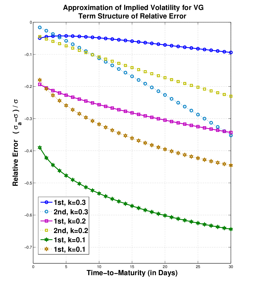
We now proceed to illustrate the performance of the implied volatility approximations described in Section 2.1. Concretely, we analyze the relative error of the approximations

\tilde{\sigma}_{t,1}(k)=\sqrt{\frac{V_{0}(t,k)}{t}},\quad\tilde{\sigma}_{t,2}(k)=\sqrt{\frac{V_{0}(t,k)(1+V_{1}(t,k))}{t}}.

(46)

Let us first analyze the Variance Gamma model with parameter values as above. The left panel of Figure 3 shows the relative errors $(\tilde{\sigma}_{t,1}-\hat{\sigma}_{t})/\hat{\sigma}_{t}$ and $(\tilde{\sigma}_{t,2}-\hat{\sigma}_{t})/\hat{\sigma}_{t}$ as a function of time-to-maturity $t$ for values of $k$ ranging from $0.1$ to $0.3$ . Note that both $\tilde{\sigma}_{t,1}$ and $\tilde{\sigma}_{t,2}$ consistently underestimate the true implied volatility. For $k=0.3$ , the first order approximation is actually quite good with a relative error of about $-5\%$ uniformly in $t$ and it is only for very small values $t$ (less than $3$ days) when $\tilde{\sigma}_{t,2}$ is better than $\tilde{\sigma}_{t,1}$ . However, for the other values of $k$ , $\tilde{\sigma}_{t,2}$ significantly outperforms $\tilde{\sigma}_{t,1}$ . For instance, for $k=0.2$ , the relative error of $\tilde{\sigma}_{t,1}$ ranges from $-19\%$ to $-34\%$ with a mean absolute error of $27.0\%$ , while the relative error of $\tilde{\sigma}_{t,2}$ rages from $-4.4\%$ to $-23\%$ with a mean absolute error of $14.2\%$ . The left panel of Figure 4 compares the term structure of the approximated implied volatilities to the ‘‘true” implied volatility³³ 3 The “true” implied volatility is actually an approximation as we apply numerical integration to compute $\mathbb{E}(S_{T}-K)_{+}$ using the closed-form density of the VG process. This approximation seems not to be very accurate for $t$ smaller than $3$ days.. The right panel of Figure 3 shows the analog results for the CGMY with parameter values as above. The results are qualitatively similar to those of the Variance Gamma model. However, all the approximations seem to perform better in terms of error stability in time and accuracy. For $k=0.2$ , the relative error of $\tilde{\sigma}_{t,1}$ ranges from $-12\%$ to $-20\%$ with a mean absolute error of $18.6\%$ , while the relative error of $\tilde{\sigma}_{t,2}$ ranges from $0.83\%$ to $-13\%$ with a mean absolute error of $9.25\%$ . The right panel of Figure 4 compares the term structure of the approximated implied volatilities to the ‘‘true” implied volatility⁴⁴ 4 The true implied volatility is computed by integrating numerically the the density of the CGMY model, which itself is obtained by Fast Fourier methods..

Acknowledgments: It is a pleasure to thank Michael Roper for pointing up several notational mistakes and other helpful comments. We would also like to thank Peter Tankov for providing us with his manuscript.

References

[AS02] Aït-Sahalia, Y., “Telling from discrete data whether the underlying continuous-time model is a diffusion”, Journal of Finance, 57, 2075-2113, 2002.
[AJ09a] Aït-Sahalia, Y. and J.Jacod, “Estimating the Degree of Activity of Jumps in High Frequency Data”, Annals of Statistics, 2009, 37, 2202-2244.
[AJ09b] Aït-Sahalia, Y. and J. Jacod, “Testing for jumps in a discretely observed process”, Annals of Statistics, 37:184-222, 2009.
[AJ10] Aït-Sahalia, Y. and J. Jacod, “Is Brownian motion necessary to model high frequency data?”, Annals of Statistics, 38, 3093-3128, 2010.
[BNS06] Barndorff-Nielsen, O. and N. Shephard, “Econometrics of testing for jumps in financial economics using bipower variation”, Journal of Financial Econometrics, 4(1):1-30, 2006.
[Bar97] Barndorff-Nielsen, O., “Normal inverse Gaussian distributions and stochastic volatility modelling”, Scand. J. Statist., 24, 1-13, 1997.
[Ber96] Bertoin, J., “Lévy processes”, Cambridge University Press, 1996.
[Bjr09] Björk, T., “Arbitrage Theory in Continuous Times”, Oxford University Press, 2009.
[BL02] Boyarchenko, S.I., and S.Z. Levendorksii, “Non-Gaussian Merton-Black- Scholes theory”, Adv. Ser. Stat. Sci. Appl. Probab. 9. World ScientiÞc Publish- ing Co., Inc., River Edge, NJ, 2002.
[CM09] Carr, P., and D. Madan, “Saddlepoint methods for option pricing”, The Journal of Computational Finance, 13(1), 49-61, 2009.
[CGMY02] Carr, P., H. Geman, D. Madan and M. Yor, “The fine structure of asset returns: An empirical investigation”, Journal of Business, 75, 303-325, 2002.
[CGMY03] Carr, P., H. Geman, D. Madan and M. Yor, “Stochastic volatility for Lévy processes”, Mathematical Finance, 13, 345-382, 2003.
[CGMY05] Carr, P., H. Geman, D. Madan and M. Yor (2005), “Pricing Options on Realized Variance”, Finance and Stochastics, 9, 453-475.
[CT04] Cont, R. and P. Tankov, “Financial modelling with Jump Processes”, Chapman & Hall, 2004.
[CW03] Carr, P. and L. Wu, “What type of process underlies options? A simple robust test”, Journal of Finance, 58, no. 6, 2581-2610, 2003.
[FL08] Figueroa-López, J., “Small-time moment asymptotics for Lévy processes”, Statistics and Probability Letters, 78, 3355-3365, 2008.
[FL10] Figueroa-López, J., “Approximations for the distributions of bounded variation Lévy processes”, Statistics and Probability Letters, 80, 1744-1757, 2010.
[FLGH11] Figueroa-López, J., R. Gong, and C. Houdré, “Small-time expansions for the distributions, densities, and option prices of stochastic volatility models with Lévy jumps”, Preprint 2011. Available at http://arxiv.org/abs/1009.4211.
[FLH09] Figueroa-López, J. and C. Houdré, “Small-time expansions for the transition distribution of Lévy processes”, Stochastic Processes and their Applications, 119 pp. 3862-3889, 2009. DOI: 10.1016/j.spa.2009.09.002.
[Forde09] Forde, M., “Small-time asymptotics for a general local-stochastic volatility model, using the heat kernel expansion”, Preprint 2009.
[Forde10] Forde, M., “Exact pricing and large-time asymptotics for the modified SABR model and the Brownian exponential functional”, Preprint 2010.
[FJL10] Forde, M., A.Jacquier and R.Lee, “The small-time smile and term structure of implied volatility under the Heston model”, Preprint 2010.
[GL11] Gao, K., and R. Lee, “Asymptotics of Implied Volatility in Extreme Regimes”, Preprint 2011. Available at http://papers.ssrn.com/.
[GHLOW09] Gatheral, J., E. Hsu, P. Laurence, C. Ouyang, and T. Wang, “Asymptotics of implied volatility in local volatility models”, to appear in Mathematical Finance, 2011.
[Hou02] Houdré, C., “Remarks on deviation inequalities for functions of infinitely divisible random vectors”, The Annals of Probability, 30(3):1223–1237, 2002.
[Kop95] Koponen, I. (1995). “Analytic approach to the problem of convergence of truncated Lévy flights towards the Gaussian stochastic process”, Physical Review E, 52, 1197-1199.
[Lee04] Lee, R.W., “Option Pricing by Transform Methods: Extensions, Unification, and Error Control”, Journal of Computational Finance, 7(3):51-86, 2004.
[Lev04a] Levendorskii, S., “American and European options near expiry, under Lévy processes”, Tech. report, The University of Texas, 2004. Available at SSRN.
[Lev04b] Levendorskii, S., “Pricing of the American put under Lévy processes”, International Journal of Theoretical and Applied Finance, 7:303Ð-335, 2004.
[Lev04c] Levendorskii, S., “Early exercise boundary and option pricing in Lévy driven models”, Quantitative Finance, 4:525-Ð547, 2004.
[Lev08] Levendorskii, S., “American and European Options in Multi-Factor Jump-Diffusion Models Near Expiry”, Finance and Stochastics, 12:4 (2008), pp.541-560.
[Man63] Mandelbrot, B., “The variation of certain speculative prices”, Journal of Business, 36:394-419, 1963.
[KRMK11] Keller-Ressel, M. and J. Muhle-Karbe, “Asymptotic and Exact Pricing of Options on Variance”, 2011, to appear in Finance and Stochastics.
[Olv74] Olver, F.W., “Asymptotics and Special Functions“, Academic Press, 1974.
[Rop10] Roper, M., “Implied volatility: small time to expiry asymptotics in exponential Lévy models”, Thesis, University of New South Wales, 2009.
[RT11] Rosenbaum, M., and P. Tankov, “Asymptotic results for time-changed Lévy processes sampled at hitting times”, Preprint. To appear in Stochastic processes and their applications, 2011.
[Ros07] Rosiński, J., “Tempering stable processes”, Stochastic processes and their applications, 117: 677-707, 2007.
[Sat99] Sato, K., “Lévy Processes and Infinitely Divisible Distributions”, Cambridge studies in advance mathematics, 1999.
[Tnkv10] Tankov, P., “Pricing and hedging in exponential Lévy models: review of recent results”, Prepint 2010. To appear in the Paris-Princeton Lecture Notes in Mathematical Finance, Springer 2010.
[Will91] Williams, D., “Probability with Martingales”, Cambridge Mathematical Textbooks, 1991.
[Win01] Winkel, M., “The recovery problem for time-changed Lévy processes”, Oxford University, 2001.

Appendix A Proofs

Proof of Theorem 2.3.

We know that $V(t,k)\to 0$ . Equating call prices in the small-time limit under the exponential Lévy model (using Proposition 2.2), and the Black-Scholes model with zero interest rates and implied variance $V=V(t,k)$ (using e.g. Proposition 3.4 in [FJL10] or Lemma 2.5 in [GHLOW09]) we know that for any $\delta>0$ , there exists a $t^{*}=t^{*}(\delta)$ such that for all $t<t^{*}$

\displaystyle ta_{0}(k)(1-\delta)\,\leq\,\frac{1}{S_{0}}\mathbb{E}(S_{t}-K)^{+}\,\leq\,e^{-\frac{1}{2}k^{2}(1-\delta)/V(t,k)}\,.

(A-1)

Re-arranging, we see that

-V(t,k)\log[ta_{0}(k)(1-\delta)]\,\geq\,\frac{1}{2}k^{2}(1-\delta)\,,

V(t,k)\cdot\log(\frac{1}{t})\,\geq\,\frac{1}{2}k^{2}(1-\delta)+V(t,k)\log(1-\delta)+V(t,k)\log a_{0}(k)\,.

$V(t,k)\to 0$ , so this yields a lower bound for $V(t,k)$ . Using a similar argument for the corresponding upper bound, we establish the leading order asymptotic behaviour for the implied variance as

V(t,k)\,\sim V_{0}(t,k):=\frac{\frac{1}{2}k^{2}}{\log(\frac{1}{t})}\quad\quad\quad\quad\quad(t\to 0)\,.

(A-2)

Now let $V(t,k)=V_{0}(t,k)\big[1+\tilde{V}_{1}(t,k)\big]\,$ and note that $\tilde{V}_{1}(t,k)=o(1)$ as $t\to{}0$ . Then for any $\delta>0$ , there exists a $t^{**}=t^{**}(\delta)$ such that for $t<t^{**}$ we have

\frac{1}{t}[\frac{1}{t}\,\frac{1}{S_{0}}\mathbb{E}(S_{t}-K)^{+}-a_{0}(k)]-a_{1}(k)\geq-\delta\,.

(A-3)

Re-arranging, we have

ta_{0}(k)+(a_{1}(k)-\delta)t^{2}\,\leq\,\frac{1}{S_{0}}\mathbb{E}(S_{t}-K)^{+}\,.

(A-4)

Using this bound and again equating small-time call prices under the Lévy model and the Black-Scholes model, we have that there exists a positive constant $c$ such that for $t$ small enough

$\displaystyle ta_{0}(k)+(a_{1}(k)-\delta)t^{2}\,\leq\,\frac{1}{S_{0}}\mathbb{E}(S_{t}-K)^{+}$	$\displaystyle\leq$	$\displaystyle\,\frac{e^{\frac{1}{2}k}V(t,k)^{\frac{3}{2}}}{\sqrt{2\pi}\,k^{2}}e^{-\frac{1}{2}k^{2}/V(t,k)}(1+cV(t,k))$
	$\displaystyle=$	$\displaystyle\frac{e^{\frac{1}{2}k}V_{0}(t,k)^{\frac{3}{2}}(1+\tilde{V}_{1}(t,k))^{\frac{3}{2}}}{\sqrt{2\pi}\,k^{2}}e^{-\frac{1}{2}k^{2}/\{V_{0}(t,k)(1+\tilde{V}_{1}(t,k))\}}(1+cV(t,k))\quad\quad\quad$
	$\displaystyle\leq$	$\displaystyle\frac{e^{\frac{1}{2}k}V_{0}(t,k)^{\frac{3}{2}}}{\sqrt{2\pi}\,k^{2}}e^{-\frac{1}{2}k^{2}/\{V_{0}(t,k)(1+\tilde{V}_{1}(t,k))\}}(1+\mathcal{E}(t,k)),\quad\quad\quad\quad\quad(t\to 0)\,.$

where $\mathcal{E}(t,k):=(1+\tilde{V}_{1}(t,k))^{3/2}(1+cV(t,k))-1$ , which converges to $0$ as $t\to{}0$ . Dividing both sides by $t=e^{-\frac{1}{2}k^{2}/V_{0}(t,k)}$ we have

a_{0}(k)+(a_{1}(k)-\delta)t\,\leq\,\frac{e^{\frac{1}{2}k}V_{0}(t,k)^{\frac{3}{2}}}{\sqrt{2\pi}\,k^{2}}\,e^{\frac{1}{2}k^{2}\tilde{V}_{1}(t,k)/\{V_{0}(t,k)(1+\tilde{V}_{1}(t,k))\}}(1+\mathcal{E}(t,k))\,,

and re-arranging we obtain

$\displaystyle\frac{\tilde{V}_{1}(t,k)}{1+\tilde{V}_{1}(t,k)}\,$	$\displaystyle\geq$	$\displaystyle\,\frac{2}{k^{2}}V_{0}(t,k)\log\big[(a_{0}(k)+(a_{1}(k)-\delta)t)\sqrt{2\pi}\,k^{2}e^{-\frac{1}{2}k}V_{0}(t,k)^{-\frac{3}{2}}/(1+\mathcal{E}(t,k))\big]\,.$
	$\displaystyle=$	$\displaystyle\,\frac{2}{k^{2}}V_{0}(t,k)\log\big[(a_{0}(k)+t\,a_{1}(k))\sqrt{2\pi}\,k^{2}e^{-\frac{1}{2}k}V_{0}(t,k)^{-\frac{3}{2}}\big]+\frac{2}{k^{2}}V_{0}(t,k)\log\big[\frac{1-\frac{\delta t}{a_{0}(k)+a_{1}(k)t}}{1+\mathcal{E}(t,k)}\big]$
	$\displaystyle=$	$\displaystyle\underbrace{\frac{1}{\log(\frac{1}{t})}\log\left[\frac{4\sqrt{\pi}a_{0}(k)e^{-k/2}}{k}[\log(\frac{1}{t})]^{\frac{3}{2}}\right]}_{V_{1}(t,k)}+\underbrace{\frac{1}{\log(\frac{1}{t})}\log\left\{\left[1+t\,\frac{a_{1}(k)}{a_{0}(k)}\right]\left[\frac{1-\frac{\delta t}{a_{0}(k)+a_{1}(k)t}}{1+\mathcal{E}(t,k)}\right]\right\}}_{\mathcal{E}^{\prime}(t,k)}\,.$

Note that $V_{1}=V_{1}(t,k)=O\left(\frac{\log\log\frac{1}{t}}{\log\frac{1}{t}}\right)$ and $\mathcal{E}^{\prime}=\mathcal{E}^{\prime}(t,k)=o(\frac{1}{\log\frac{1}{t}})$ since $\mathcal{E}(t,k)\to{}0$ as $t\to{}0$ . Solving the inequality $\frac{\tilde{V}_{1}}{1+\tilde{V}_{1}}\geq V_{1}+\mathcal{E}^{\prime}$ , we find that

\tilde{V_{1}}\,\geq\,\frac{V_{1}+\mathcal{E}^{\prime}}{1-(V_{1}+\mathcal{E}^{\prime})}=V_{1}+\mathcal{E}^{\prime}+\frac{V_{1}^{2}+2V_{1}\mathcal{E}^{\prime}+\mathcal{E}^{\prime}{}^{2}}{1-(V_{1}+\mathcal{E}^{\prime})}.

Since $\mathcal{E}^{\prime}(t,k)>V^{2}_{1}(t,k)$ for $t$ sufficiently small, we conclude that $\tilde{V_{1}}\,\geq V_{1}+o(\frac{1}{\log\frac{1}{t}})$ . Proceeding similarly for the upper bound, we conclude that

\tilde{V}_{1}(t,k)=V_{1}(t,k)+o(\frac{1}{\log\frac{1}{t}})\,.

as $t\to 0$ . ∎

Proof of Theorem 3.2.

Let $\bar{F}(t):=\mathbb{P}(X_{t}\geq{}x)$ and $B:=\nu[x,\infty)+\sup_{t>0}\mathbb{P}(X_{t}\geq{}x)/t$ . In the light of Theorem 2.1, there exist constants $t_{0}>0$ and $K<\infty$ such that

\left|\frac{1}{t}\mathbb{P}(X_{t}\geq{}x)-\nu[x,\infty)\right|\leq Kt,

for any $0<t<t_{0}$ . Next, conditioning on $T_{t}$ ,

\displaystyle\frac{1}{t}\,\mathbb{P}(X_{T_{t}}\geq{}x)=\frac{1}{t}\,\mathbb{E}\,\bar{F}(T_{t})=\frac{\nu[x,\infty)}{t}\,\mathbb{E}\,T_{t}+\frac{1}{t}\,\mathbb{E}\left(\left\{\frac{1}{T_{t}}\bar{F}(T_{t})-\nu[x,\infty)\right\}T_{t}\right).

Let $R_{2}(t)$ denote the second term on the right-hand side, which we can bound as follows:

	$\displaystyle\|R_{2}\|$	$\displaystyle\leq\frac{1}{t}\,\mathbb{E}\left(1_{\{T_{t}<t_{0}\}}\left\|\frac{1}{T_{t}}\bar{F}(T_{t})-\nu[x,\infty)\right\|T_{t}\right)+\frac{1}{t}\,\mathbb{E}\left(\,1_{\{T_{t}\geq t_{0}\}}\left\|\frac{1}{T_{t}}\bar{F}(T_{t})-\nu[x,\infty)\right\|T_{t}\right)$
		$\displaystyle\leq K\frac{1}{t}\mathbb{E}\,T^{2}_{t}+B\frac{1}{t}\mathbb{E}(\,1_{\{T_{t}\geq t_{0}\}}T_{t})\leq K\frac{1}{t}\mathbb{E}\,T^{2}_{t}+\frac{B}{t_{0}}\frac{1}{t}\mathbb{E}\,(T_{t}^{2}),$

using a Chebyshev upper bound. Combining the previous bounds, we have

	$\displaystyle\frac{1}{t}\left\|\frac{1}{t}\,\mathbb{P}(Z_{t}\geq{}x)-\mathbb{E}Y_{0}\nu[x,\infty)\right\|$	$\displaystyle\leq\frac{\nu[x,\infty)}{t}\left\|\frac{1}{t}\mathbb{E}T_{t}-\mathbb{E}Y_{0}\right\|+\frac{K}{t^{2}}\mathbb{E}\,(T^{2}_{t})+\frac{B}{t_{0}}\frac{1}{t^{2}}\mathbb{E}\,(T_{t}^{2})$
		$\displaystyle\leq\frac{\nu[x,\infty)}{t^{2}}\int_{0}^{t}\left\|\mathbb{E}Y_{s}-\mathbb{E}Y_{0}\right\|ds+\frac{K}{t^{2}}\mathbb{E}(T_{t}^{2})+\frac{B}{t_{0}}\frac{1}{t^{2}}\mathbb{E}(T_{t}^{2})$

Next, (26) and Jensen’s inequality imply that

\displaystyle\limsup_{t\to{}0}\frac{1}{t^{2}}\int_{0}^{t}\left|\mathbb{E}Y_{s}-\mathbb{E}Y_{0}\right|ds<\infty,\quad\limsup_{t\to{}0}\frac{1}{t^{2}}\mathbb{E}(T_{t}^{2})\leq\limsup_{t\to{}0}\frac{1}{t}\int_{0}^{t}\mathbb{E}Y^{2}_{s}ds<\infty,

and (28) will follow. In order to show (29), consider now

G_{x}(t):=\frac{1}{t}\left\{\frac{1}{t}\mathbb{P}(X_{t}\geq{}x)-\nu[x,\infty)\right\}-\frac{d_{2}(x)}{2},

and note that, in view of Theorem 2.1, there exist constants $t_{0}(\varepsilon)>0$ and $K\in(0,\infty)$ such that

\sup_{t>0}|G_{x}(t)|\leq K,\quad\text{and}\quad|G_{x}(t)|<\varepsilon,

for any $0<t<t_{0}$ . As before,

	$\displaystyle\frac{1}{t^{2}}\mathbb{P}(Z_{t}\geq{}x)$	$\displaystyle=\frac{1}{t^{2}}\mathbb{E}\bar{F}(T_{t})=\frac{1}{t^{2}}\,\mathbb{E}\left(\left\{\frac{1}{T_{t}}\bar{F}(T_{t})-\nu[x,\infty)\right\}T_{t}\right)+\frac{\nu[x,\infty)}{t^{2}}\,\mathbb{E}\,T_{t}$
		$\displaystyle=\frac{1}{t^{2}}\,\mathbb{E}\left(G_{x}(T_{t})T_{t}^{2}\right)+\frac{d_{2}(x)}{2t^{2}}\,\mathbb{E}(T_{t}^{2})+\frac{\nu[x,\infty)}{t^{2}}\,\mathbb{E}\,T_{t}\,.$

The first term in the last expression can be bounded as follows:

	$\displaystyle\left\|\frac{1}{t^{2}}\,\mathbb{E}\left(G_{x}(T_{t})T_{t}^{2}\right)\right\|$	$\displaystyle\leq\left\|\frac{1}{t^{2}}\,\mathbb{E}\left(1_{\{T_{t}<t_{0}\}}G_{x}(T_{t})T_{t}^{2}\right)\right\|+\left\|\frac{1}{t^{2}}\,\mathbb{E}\left(1_{\{T_{t}\geq t_{0}\}}G_{x}(T_{t})T_{t}^{2}\right)\right\|$
		$\displaystyle\leq\frac{\varepsilon}{t^{2}}\mathbb{E}\,(T_{t}^{2})+K\frac{1}{t^{2}}\mathbb{E}(\,1_{\{T_{t}\geq t_{0}\}}T_{t}^{2}).$

Then, it is now clear that we can bound the expression

\displaystyle D_{t}:=\left|\frac{1}{t^{2}}\mathbb{P}(Z_{t}\geq{}x)-\frac{1}{t}\mathbb{E}Y_{0}\nu[x,\infty)-\frac{\rho d_{2}(x)}{2}-{\frac{\gamma\nu[x,\infty)}{2}}\right|,

as follows

\displaystyle D_{t}\leq\varepsilon\frac{1}{t^{2}}\mathbb{E}(T_{t}^{2})+K\frac{1}{t^{2}}\mathbb{E}(T^{2}_{t}1_{\{T_{t}\geq{}t_{0}\}})+\nu[x,\infty)\left|{\frac{1}{t}\left(\frac{1}{t}\mathbb{E}T_{t}-\mathbb{E}Y_{0}\right)-\frac{\gamma}{2}}\right|+\frac{|d_{2}(x)|}{2}\left|\frac{1}{t^{2}}\mathbb{E}(T_{t}^{2})-\rho\right|.

The third term on the right hand side of the above inequality is such that

\displaystyle\frac{1}{t}\left(\frac{1}{t}\mathbb{E}T_{t}-\mathbb{E}Y_{0}\right)-\frac{\gamma}{2}=\frac{1}{t^{2}}\int_{0}^{t}s\left\{\frac{1}{s}(\mathbb{E}Y_{s}-\mathbb{E}Y_{0})-\gamma\right\}ds,

which converges to $0$ as $t\to{}0$ due to (iii) in (26). Hence, using (iv)-(v) in (27) and

\mathbb{E}(T^{2}_{t}1_{\{T_{t}\geq{}t_{0}\}})\leq\mathbb{E}(T^{3}_{t})/t_{0}\leq t^{2}\int_{0}^{t}\mathbb{E}(Y_{s}^{3})ds/t_{0},

we have

\limsup_{t\to{}0}D_{t}\leq\varepsilon\rho,

which implies (29) because $\varepsilon$ is arbitrary. ∎

Proof of Lemma 4.3.

We start by introducing some notation. Suppose that, under $\mathbb{P}^{*}$ , $X$ has Lévy-Itô decomposition

{X}_{t}=b^{*}t+\int_{0}^{t}\int_{|z|\leq{}1}z\,\bar{\mu}^{*}(dz,ds)+\int_{0}^{t}\int_{|z|>1}z\,\mu^{*}(dz,ds),

(A-5)

where $\mu^{*}$ is an independent Poisson measure on $\mathbb{R}\backslash\{0\}\times\mathbb{R}_{+}$ with mean measure $\nu^{*}(dz)dt$ , and $\bar{\mu}^{*}(dz,dt):=\mu^{*}(dz,dt)-\nu^{*}(dz)dt$ . Next, for a given fixed $\varepsilon>0$ , we set

\displaystyle\widetilde{{X}}^{\varepsilon}_{t}:=\int_{0}^{t}\int_{\mathbb{R}}z\,{\bf 1}_{\{|z|\geq{}\varepsilon\}}\mu^{*}(dz,ds),\quad\text{ and }\quad{X}^{\varepsilon}_{t}:={X}_{t}-\widetilde{{X}}^{\varepsilon}_{t};

(A-6)

hence, $\widetilde{{X}}^{\varepsilon}$ is a compound Poisson process with intensity $\lambda_{\varepsilon}:=\nu^{*}(|z|\geq{}\varepsilon)$ and jumps $\{\xi_{i}^{\varepsilon}\}_{i}$ with common distribution ${\bf 1}_{|z|\geq{}\varepsilon}\nu^{*}(dz)/\lambda_{\varepsilon}$ , while the remainder process ${X}^{\varepsilon}$ is a Lévy process with triplet $(0,b_{\varepsilon}^{*},{\bf 1}_{\{|z|\leq{}\varepsilon\}}\nu^{*}(dz))$ , where

b_{\varepsilon}^{*}:=b^{*}-\int_{|z|\leq{}1}z{\bf 1}_{\{|z|\geq{}\varepsilon\}}\nu^{*}(dz).

Let us fixed $\varepsilon=x/2$ . We first note that

\mathbb{P}^{*}\left(\widetilde{X}^{\varepsilon}_{t}\geq{}x\right)\leq{}Kx^{-Y}t,

for any $t,x>0$ and for some universal constant $K$ . Indeed, if we let $N^{\varepsilon}_{t}$ denote the number of jumps before time $t$ of the compound Poisson process $\widetilde{X}^{\varepsilon}$ , then we have

\displaystyle\mathbb{P}^{*}\left(\widetilde{X}^{\varepsilon}_{t}\geq{}x\right)

\displaystyle\leq\mathbb{P}^{*}\left(N^{\varepsilon}_{t}\neq{}0\right)=1-e^{-\lambda_{\varepsilon}t}\leq\lambda_{\varepsilon}t=\nu(\{z:|z|\geq x/2\})t\leq Cx^{-Y}t.

We now estimate $\mathbb{P}^{*}\left({X}^{\varepsilon}_{t}\geq{}x\right)$ . First, note that, due to the symmetry of the Lévy measure $\nu$ ,

	$\displaystyle\mathbb{E}^{*}(X_{t}^{\varepsilon})$	$\displaystyle=t(b^{}_{\varepsilon}+\int_{\|z\|\geq{}1}z{\bf 1}_{\{\|z\|\leq{}\varepsilon\}}\nu^{}(dz))=t(b^{*}-\int_{\|z\|\leq{}1}z{\bf 1}_{\{\|z\|\geq{}\varepsilon\}}e^{z}\nu(dz)+\int_{\|z\|\geq{}1}z{\bf 1}_{\{\|z\|\leq{}\varepsilon\}}e^{z}\nu(dz))$
		$\displaystyle=t(b+\int_{\|z\|\leq{}1}z(e^{z}-1)\nu(dz)-\int_{\|z\|\leq{}1}z{\bf 1}_{\{\|z\|\geq{}\varepsilon\}}e^{z}\nu(dz)+\int_{\|z\|\geq{}1}z{\bf 1}_{\{\|z\|\leq{}\varepsilon\}}e^{z}\nu(dz))$
		$\displaystyle=t(b+\int_{\|z\|\leq{}\varepsilon}z(e^{z}-1)\nu(dz))=t(b+\int_{\|z\|\leq{}x/2}z(e^{z}-1)\nu(dz)).$

Thus, using concentration inequalities for centered random variable (e.g. [Hou02], Corollary 1), for $x>2\mathbb{E}X_{t}^{\varepsilon}$ ,

\displaystyle\mathbb{P}^{*}({X}_{t}^{\varepsilon}\geq x)\leq\mathbb{P}^{*}({X}_{t}^{\varepsilon}-\mathbb{E}^{*}{X}_{t}^{\varepsilon}\geq x/2)\leq{e^{\frac{x}{2\varepsilon}-\left(\frac{x}{2\varepsilon}+\frac{tV_{\varepsilon}^{2}}{\varepsilon^{2}}\right)\log\left(1+\frac{\varepsilon x}{2tV_{\varepsilon}^{2}}\right)}}\leq\left(\frac{2eV_{\varepsilon}^{2}}{\varepsilon x}\right)^{\frac{x}{2\varepsilon}}t^{\frac{x}{2\varepsilon}}\leq\frac{4V_{x/2}^{2}}{x^{2}}t,

where $V_{\varepsilon}^{2}:={\rm Var}^{*}(X_{1}^{\varepsilon})=\int_{\{|z|\leq{}\varepsilon\}}z^{2}\nu^{*}(dz)$ . Since $M>1$ , there exists a universal constant $K$ such that

	$\displaystyle\frac{V_{x/2}^{2}}{x^{2}}$	$\displaystyle=\frac{C\int_{0}^{x/2}\frac{e^{-(G-1)z}}{z^{1+Y}}z^{2}dz}{x^{2}}+\frac{C\int_{0}^{x/2}\frac{e^{-(M-1)z}}{z^{1+Y}}z^{2}dz}{x^{2}}$
		$\displaystyle\leq\frac{2C\int_{0}^{x/2}z^{1-Y}dz}{x^{2}}=\frac{2C(x/2)^{2-Y}}{(2-Y)x^{2}}=Kx^{-Y}.$

We conclude that $\mathbb{P}^{*}({X}_{t}^{\varepsilon}\geq x)\leq Ktx^{-Y}$ for $t(b+\int_{|z|\leq{}x/2}z(e^{z}-1)\nu(dz))<x/2$ . This completes the proof, since

\mathbb{P}^{*}(X_{t}\geq{}x)\leq\mathbb{P}^{*}(X_{t}^{\varepsilon}\geq{}x/2)+\mathbb{P}^{*}(\widetilde{X}^{\varepsilon}_{t}\geq{}x/2)\leq Ktx^{-Y},

whenever $t(b+\int_{|z|\leq{}x/4}z(e^{z}-1)\nu(dz))<x/4$ . ∎

Proof of Proposition 4.2.

Without loss of generality, we assume $S_{0}=1$ . We break the proof into two parts:

(1) Let us assume through this part that $(X_{t})_{t}$ is a symmetric CGMY process. Let $b(u):=b+\int_{|z|\leq{}u}z(e^{z}-1)\nu(dz)$ . Obviously,

\displaystyle b(u)\leq|b(u)|\leq|b|+\int_{|z|\leq{}1}|z||e^{z}-1|\nu(dz)+2\int_{|z|\geq{}1}|z|e^{z}\nu(dz):=\bar{b}<\infty.

(A-7)

Next, we write

	$\displaystyle\int_{0}^{\infty}e^{-t^{1/Y}u}\mathbb{P}^{*}\left(X_{t}\geq{}t^{1/Y}u\right)du$	$\displaystyle=\int_{0}^{\infty}{\bf 1}_{\{{u/4}\leq t^{1-1/Y}\bar{b}\}}e^{-t^{1/Y}u}\mathbb{P}^{*}\left(X_{t}\geq{}t^{1/Y}u\right)du$		(A-8)
		$\displaystyle+\int_{0}^{\infty}{\bf 1}_{\{{u/4}>t^{1-1/Y}\bar{b}\}}e^{-t^{1/Y}u}\mathbb{P}^{*}\left(X_{t}\geq{}t^{1/Y}u\right)du.$		(A-9)

Clearly, $e^{-t^{1/Y}u}\mathbb{P}^{*}\left(X_{t}\geq{}t^{1/Y}u\right)\leq 1$ , so the first term converges to $0$ as $t\to{}0$ because $Y\in(1,2)$ . From the inequality (A-7), we have

{\bf 1}_{\left\{{u/4}>t^{1-1/Y}\bar{b}\right\}}={\bf 1}_{\left\{t^{1/Y}u>t\bar{b}\right\}}\leq{\bf 1}_{\left\{t^{1/Y}{u/4}>t{b}(t^{1/Y}u/4)\right\}},

and using Lemma 4.3, we obtain that

	$\displaystyle{\bf 1}_{\left\{{u/4}>t^{1-1/Y}\bar{b}\right\}}e^{-t^{1/Y}u}\mathbb{P}^{*}\left(X_{t}\geq{}t^{1/Y}u\right)$	$\displaystyle\leq{\bf 1}_{\left\{t^{1/Y}{u/4}>t{b}\left(t^{1/Y}u/4\right)\right\}}e^{-t^{1/Y}u}\mathbb{P}^{*}\left(X_{t}\geq{}t^{1/Y}u\right)$
		$\displaystyle\leq\min\{K(t^{1/Y}u)^{-Y}t,1\}=\min\{Ku^{-Y},1\},$

which is integrable because $Y\in(1,2)$ . Hence, we can apply dominated convergence in the second term (A-9) and, using Proposition 4.1, we obtain that

\lim_{t\to{}0}\int_{0}^{\infty}e^{-t^{1/Y}u}\mathbb{P}^{*}\left(X_{t}\geq{}t^{1/Y}u\right)du=\int_{0}^{\infty}\mathbb{P}^{*}(Z\geq{}u)du=\mathbb{E}^{*}(Z_{+}).

This show the result in view of (39)-(40).

(2) In this second part, we relax the symmetry restriction. The idea is to reduce the problem to the symmetric case by applying a change of probability measure.⁵⁵ 5 A similar argument is applied in the proof of Proposition 5-(2) in [Tnkv10] but with a different aim. Concretely, let $\beta:=\frac{M-G}{2}$ and, as in the proof of Proposition 2.2, define a probability measure $\widehat{\mathbb{P}}$ on $(\Omega,\mathcal{F})$ such that

\widehat{\mathbb{P}}(B)=\mathbb{E}\left(e^{\beta X_{t}}1_{B}\right)/\mathbb{E}\left(e^{\beta X_{t}}\right),

(A-10)

for any $B\in\mathcal{F}_{t}$ . We can check that, under $\widehat{\mathbb{P}}$ , $(X_{t})_{t}$ is a symmetric CGMY model with $\hat{C}=C$ , $\hat{Y}=Y$ , and $\hat{G}=\hat{M}=(M+G)/2$ . Indeed, it follows that

	$\displaystyle\hat{\mathbb{E}}\left(e^{iuX_{t}}\right)$	$\displaystyle=\mathbb{E}\left(e^{(iu+\beta)X_{t}}\right)/\mathbb{E}\left(e^{\beta X_{t}}\right)$
		$\displaystyle=\exp\left[t\,C\Gamma(-Y)\left\{(M-\beta-iu)^{Y}+(G+\beta+iu)^{Y}-(M-\beta)^{Y}-(G+\beta)^{Y}\right\}+i\hat{b}ut\right].$

Also, assuming $\beta>0$ ,

\displaystyle\left|{\mathbb{E}}\left(\left(e^{X_{t}}-1\right)_{+}e^{\beta X_{t}}\right)-\mathbb{E}\left(e^{X_{t}}-1\right)_{+}\right|={\mathbb{E}}\left(\left(e^{X_{t}}-1\right)_{+}\left(e^{\beta X_{t}}-1\right)\right)\leq{\mathbb{E}}\left(\left(e^{X_{t}}-1\right)\left(e^{\beta X_{t}}-1\right)\right)=O(t),

since the moment function $\varphi(x):=\frac{1}{\beta}(e^{x}-1)(e^{\beta x}-1)\sim x^{2}$ and Theorem 1.1-(ii) in [FL08] can be applied. If $\beta<0$ , then

\displaystyle\left|{\mathbb{E}}\left(\left(e^{X_{t}}-1\right)_{+}e^{\beta X_{t}}\right)-\mathbb{E}\left(e^{X_{t}}-1\right)_{+}\right|={\mathbb{E}}\left(\left(e^{X_{t}}-1\right)_{+}\left(1-e^{\beta X_{t}}\right)\right)\leq{\mathbb{E}}\left(\left(e^{X_{t}}-1\right)\left(1-e^{\beta X_{t}}\right)\right)=O(t),

for the same reason. Then, we only need to consider the asymptotic behavior of ${\mathbb{E}}\left(\left(e^{X_{t}}-1\right)_{+}e^{\beta X_{t}}\right)$ as $t\to{}0$ , because $Y\in(1,2)$ so the $O(t)$ terms above are smaller than $O(t^{1/Y})$ . However,

{\mathbb{E}}\left(\left(e^{X_{t}}-1\right)_{+}e^{\beta X_{t}}\right)=\mathbb{E}\left(e^{\beta X_{t}}\right)\widehat{\mathbb{E}}\left(\left(e^{X_{t}}-1\right)_{+}\right),

and thus, using the fact that $(X_{t})_{t}$ is symmetric under $\widehat{\mathbb{P}}$ and part (1) in this proof,

\displaystyle\lim_{t\to{}0}t^{-1/Y}{\mathbb{E}}\left(\left(e^{X_{t}}-1\right)_{+}e^{\beta X_{t}}\right)=\lim_{t\to{}0}t^{-1/Y}\widehat{\mathbb{E}}\left(\left(e^{X_{t}}-1\right)_{+}\right)=\mathbb{E}^{*}(Z_{+}).

∎

	$\displaystyle\mathbb{E}^{*}(X_{t}^{\varepsilon})$	$\displaystyle=t(b^{}_{\varepsilon}+\int_{\|z\|\geq{}1}z{\bf 1}_{\{\|z\|\leq{}\varepsilon\}}\nu^{}(dz))=t(b^{*}-\int_{\|z\|\leq{}1}z{\bf 1}_{\{\|z\|\geq{}\varepsilon\}}e^{z}\nu(dz)+\int_{\|z\|\geq{}1}z{\bf 1}_{\{\|z\|\leq{}\varepsilon\}}e^{z}\nu(dz))$
		$\displaystyle=t(b+\int_{\|z\|\leq{}1}z(e^{z}-1)\nu(dz)-\int_{\|z\|\leq{}1}z{\bf 1}_{\{\|z\|\geq{}\varepsilon\}}e^{z}\nu(dz)+\int_{\|z\|\geq{}1}z{\bf 1}_{\{\|z\|\leq{}\varepsilon\}}e^{z}\nu(dz))$
		$\displaystyle=t(b+\int_{\|z\|\leq{}\varepsilon}z(e^{z}-1)\nu(dz))=t(b+\int_{\|z\|\leq{}x/2}z(e^{z}-1)\nu(dz)).$