Spectral Singularities and Zero Energy Bound States
Abstract
Single particle scattering around zero energy is re-analysed in view of recent experiments with ultra-cold atoms, nano-structures and nuclei far from the stability valley. For non-zero orbital angular momentum the low energy scattering cross section exhibits dramatic changes depending on the occurrence of either a near resonance or a bound state or the situation in between, that is a bound state at zero energy. Such state is singular in that it has an infinite scattering length, behaves for the eigenvalues but not for the eigenfunctions as an exceptional point and has no pole in the scattering function. These results should be observable whenever the interaction or scattering length can be controlled.
pacs
03.65.Nk,34.50.-sI Introduction
Experimental techniques are nowadays capable to discern subtle phenomena in a great variety of fields of physics. Considerable progress has been made in controlling the interaction of trapped fermions providing a unique opportunity for the study of different states of the same atomic system under variation of the atomic interaction. This is achieved by means of Feshbach resonance techniques [1] using an external magnetic field; the method allows changing the scattering length in a wide range between negative and positive values. In close vicinity of the resonance or a molecular state (a halo dimer) the scattering length is very large and changes sign when going from the resonance to the molecular state.
A Bose-Einstein condensate of neutral atoms with induced electromagnetic attractive () interaction has been discussed recently as another system allowing a tunable interaction [2]. The Gross-Pitaevskii equations describing this system at a large critical negative scattering length yield the effective absorbing potential. This critical value where the onset of the collapse of the condensate occurs could be interpreted as a transition point from separate atoms to the formation of molecules or clusters [3]. In optics, using media with complex refractive index [4, 5], an abrupt phase transition has been demonstrated. It is associated with the appearance of non-orthogonal super-modes near spectral singularities, so-called exceptional points (EP) [6, 7]. Nano-structure devices provide another example, where the presence of a quasi-bound state - resonantly interacting with the continuum of scattering states - leads to a Fano-Feshbach resonance at specific system parameters [8]. All these phenomena can be explained by an effective theory of open systems described by a non-Hermitian Hamiltonian, where complex eigenstates can have square root branch points, i.e. EPs.
We recall that an EP is a singularity of a non-Hermitian Hamiltonian where eigenvalues and eigenstates coalesce. The properties of EPs were studied in earlier experiments using micro-wave cavities [9]. In many cases these singularities produce dramatic deviations from the traditional resonance behaviour, for instance a particularly strong dependence on the interaction strength (or scattering length) (see e.g. [10, 11] and papers quoted therein). Even in nuclear physics where an experimental manipulation of, say, the scattering length appears impossible, an understanding of properties of weakly bound nuclei in terms of these singularities is being approached [12]. Also, using a two-state model it was demonstrated that a non-Hermitian Hamiltonin can generate the binding of unstable states [13]; the model mimics the properties of halo nuclei which form the boundaries for a nuclear valley of stability. A kind of unification of nuclear structure and reactions based on an effective non-Hermitian Hamiltonian has been suggested to understand the transition of the nuclear chart from unbound to bound limit and vice versa [14].
The focus of the present paper lies on the singular behaviour of the energy eigenstates when the interaction (or scattering length) is varied around a bound state at zero energy. For the energies behave as if the zero energy bound state was an EP; yet the eigenfunctions and thus the scattering matrix do not share the singular behaviour. Nevertheless, the effect upon the cross section is rather dramatic, especially for . There the low energy cross section ’snaps’ from an behaviour to a behaviour when a bound state and an antibound state coalesce at (or likewise when a resonant state moves to ).
II Resumé of known facts
It is well known [15] that the single particle scattering problem with a radial potential that admits bound states can - for angular momentum larger than zero - have resonances near to zero energy. By increasing the (attractive) potential strength this resonance state evolves via a zero energy eigenstate to a bound state. Actually, both the resonance and the bound state appear as a pole of the scattering function in the complex -plane ( with the energy). In fact, a resonance gives rise to two poles in the lower -plane that are symmetrically situated with respect to the imaginary -axis. When increasing the potential strength the two resonance poles in the lower -plane move toward where they coalesce and then continue moving away at right angle in opposite directions along the imaginary -axis. The poles on the positive and negative imaginary -axis correspond to a bound and (usually denoted as) anti-bound state, respectively. Note that the wave functions associated with the resonances and the anti-bound state increase exponentially at large distance; they are the Gamow states [16]. Although these facts are well known, the aspect of the coalescence at for specific potential parameters has - to the best of our knowledge - not been sufficiently appreciated. We use the term coalescence as the merging of the two eigenvalues does not give rise to the usual degeneracy being characterised by two independent eigenfunctions. The type of singularity encountered here appears to be an EP for the eigenvalues. It therefore produces physically dramatic effects. However, as shown below, when looking at the eigenstates and the scattering function the behaviour is remarkably different from a genuine EP as it occurs generically in finite dimensional matrix problems [17].
Without specifying the potential the wave functions are not known except for their asymptotic behaviour. For potentials vanishing faster than at large distances, the asymptotic behaviour of the zero energy bound state wave function is for orbital angular momentum
| (1) |
General statements are known for the behaviour of the scattering length, the phase shift and the cross section at low energies. For non-zero energy eigenvalues the scattering length is defined by the expansion
| (2) |
where is the scattering phase shift and is proportional to the cross section. It is further known that for the case of a low energy resonance and that tends to infinity for a zero energy eigenvalue. Similarly, it is known that when a bound state has just emerged. In other words, the scattering length has a first order pole when an eigenvalue occurs at .
What happens to Eq.(2) in this latter situation? We now turn to this question.

III Analytic treatment
The motion of the poles of the scattering function, that is of the eigenvalues of the Schrödinger equation using outgoing wave boundary conditions, seem to indicate the typical signature of an EP at : a square root singularity in the potential strength. Given the potential strength that produces a bound state at for angular momentum , changing the potential to yields the new eigenvalues as
| (3) |
with finite radius of convergence. The labels 1 and 2 refer to the two resonances for ; accordingly, for and are the bound and anti-bound states energies, respectively. Note that for while are complex for . The occurrence of the square root in (3) is clearly reminiscent of an EP and also clearly signals the sprouting out of the two energies in different directions depending on the sign of . We stress that the square root behaviour in (3) refers to the eigenvalues as a function of the potential strength. Associating for the scattering function - as usually - the upper/lower -plane with the first/second sheet of the energy plane, respectively, we clearly see that an emerging bound state - a pole of the scattering function in the first energy sheet at - will always have an antibound state - a pole in the second sheet at - as a partner.
We illustrate this result explicitly for a square well of width and . In this case the -wave bound state at appears for . One finds the explicit expansions
| (4) | |||||
| (5) |
indicating nicely the motion of the levels (the poles of ) when changes from small negative to positive values as illustrated in Fig.1.
In a similar way one finds for the expansion of the scattering function around
| (6) |
while (2) remains valid for . We note that for the leading power of in (4) and (5) persists while that of (6) is to be replaced by .
IV Singularity and observable consequences
This last result invokes dramatic consequence for low energy scattering. It is illustrated in Fig.2, where the cross section

- being proprtional to - is drawn for (straight line), for (sharp rising curve) and (lower curve). Only when is the low energy cross section a constant in the energy (we simply consider the cross section integrated over the angles). As soon as the cross section starts at zero and rises with the quadratic power irrespective of the sign of . This dramatic change at low energy scattering should be observable whenever the potential or scattering length can be controlled as in the experiments discussed in the introduction. The cross sections for the different signs of are almost identical for small values of energy. The onset of the sharp rise for with increasing energy is due to the resonance generated by the slightly less attractive potential. This rise depends directly upon the magnitude of the negative value of : the smaller the smaller the resonance energy, that is the nearer to zero the occurrence of the sharp rise; yet the initial rise still remains .
This sudden switch in the low energy behaviour is a manifestation of the specific singularity for the zero energy bound state. Yet, while the spectrum appears to have the signature of an EP, neither the wave function and hence the scattering function displays the typical characteristics of an EP. In fact, while the resonances and the bound and anti-bound states are represented by a first order pole of , the two residues (the spectroscopic factors) conspire in the limit such that the pole does not occur for the bound state at zero energy. In other words, the spectroscopic factors vanish when the zero energy bound state is approached. This is in sharp contrast to the behaviour of a genuine EP in finite matrix models or for the coalescence of two resonances at a complex energy. There the scattering function (or Green’s function) has a pole of second order [18, 10]. The double pole is related to the vanishing norm of the coalescing eigenfunctions at the EP (sometimes referred to as self-orthogonality [19]). In other words, there the spectroscopic factors become large in close vicinity of an EP [14]. In the present case, the zero energy bound state wave function is normalisable. Therefore, even though the energies appear to behave like the levels at an EP including the singular behaviour, the eigenfunctions do not. Note that an EP cannot appear for a self-adjoint Hamiltonian, and the zero energy bound state problem falls into this class.
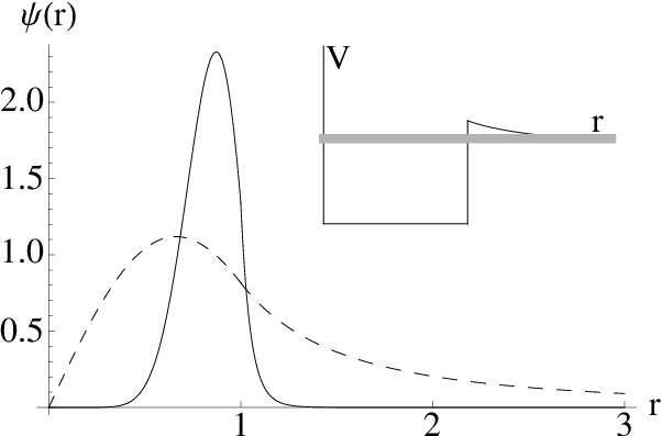
We emphasise that our findings are expected to be valid irrespective of the particular form of the radial potential as long as it falls off faster than and is less singular than at . In particular, the results are valid for an effective single particle problem describing nucleon-nucleus scattering. It is here where our results are expected to have a bearing even in nuclear physics. Note that the bound state at zero energy is “loosely” bound as seen by the mild decrease of the wave function. As stated above the state has all characteristics of a Feshbach resonance; in fact the slightest change of external parameters (scattering length) may turn it into a proper resonance or a weakly bound state. Of course, in nuclear physics the only change of parameters is moving along the isotopic or isotonic line. The situation discussed resembles that of nuclei on the drip line. In connection with halo nuclei we stress that our findings are valid for any angular momentum larger than zero. We recall in this context that the wave function for a zero energy bound state is - for higher partial waves - sharply concentrated at the surface of the binding potential, the more so the larger the angular momentum. In Fig.3 we illustrate the zero energy bound states for and . The inset shows schematically the potential indicating the role of the centrifugal part of the potential. The thick grey line indicates the energy region in which we concentrate our discussion of such Feshbach resonance. There the dramatic features for low energy scattering under variation of, for instance, the scattering length or the potential depth do occur, as has been discussed above in more detail.
In passing we note a mathematical subtlety. Even though the wave function of the anti-bound state cannot be normalised (it grows exponentially like the resonance states), we may calculate the scalar product of the bound state and the anti-bound state wave function. The exponential decay of the bound state wave function outweighs the exponential growth of the anti-bound state. As a result the integral converges and is exactly zero: the bound state is “orthogonal” upon the anti-bound state. It looks like a contradiction as the anti-bound- and bound state become the more alike the smaller . The apparent contradiction is due to the non-uniform behaviour related to the singular behaviour: the exponential growth of the anti-bound state is shifted to infinity when ; if the limit is taken before integration the scalar product does not vanish; it is the integral over the far outside tail that brings about the cancellation with the first finite part of the integral. Explicit expressions are given in the Appendix.
We suggest that, similar to the Gamow resonance states, the anti-bound wave function can have a physical meaning. Matrix elements describing transitions containing resonance states are widely used. In a similar vein the anti-bound state may be viewed as a resonance at zero frequency with a finite width. With experimental techniques available nowadays this could be within reach. We recall that the significance of an s-wave anti-bound state is known since long for the neutron-neutron system [20].
V Conclusion
To summarise, we have shown that at low energy single particle scattering for angular momentum larger than zero there is a dramatic difference for the cross section between the special situation of a zero energy bound state and the existence of either a resonance or a bound state at finite energy. For the cross section is constant in the case of a zero energy bound state, while it obeys a quadratic energy dependence for low energy eigenstates with nonzero energy (resonance or bound state). While these results have been known in principle [21], the connection to a specific singularity has - to the best of our knowledge - not been made. In fact, it is remarkable that the scattering function has no pole at a resonance at zero frequency whereas the cross section remains finite. We note that for the pattern for the cross section translates into a behaviour for the zero energy bound state and into a behaviour for the non-zero eigenvalues. We think that our findings are relevant, for instance, for experiments with trapped ultra-cold atoms in either fermion and boson gases, where the scattering length can be controlled near the threshold energy. We believe that the insights gained also have a bearing for the understanding of nuclei around the drip line where weakly bound states and larger angular momenta are relevant.
Acknowledgements
This work is partly supported by JINR-SA Agreement on scientific collaboration, by Grant No. FIS2008-00781/FIS (Spain), and by the RFBR Grant No.11-02-00086 (Russia).
Appendix
For the asymptotic behaviour of the bound state wave function is for large distances
and for the antibound state
with . Obviously the two functions become identical for . We consider the integral giving the scalar product. The tail end section (being the range from the zero of at to infinity) reads
It remains finite in the limit since remains finite (implying ) as seen from (3); an example is given in (4) and (5) when the limits are taken for and . Note that the integral above would vanish if the limit is taken before integration. For it is the finite value of the tail end integral that cancels against the first part of the scalar product integration thus causing “orthogonality” of and for . Yet, when the two functions are identical and have a finite norm.
References
- [1] C. Chin, R. Grimm, P. Julienne, and E. Tiesinga, Rev. Mod. Phys. 82, 1225 (2010).
- [2] I. Papadopoulos, P. Wagner, G. Wunner, and J. Main, Phys. Rev. A76, 053604 (2007).
- [3] H. Cartarius, J. Main, and G. Wunner, Phys. Rev. A77, 013618 (2008).
- [4] A. Guo, G. J. Salamo, D. Duchesne, R. Morandotti, M. Volatier-Ravat, V. Aimez, G. A. Siviloglou, and D. N. Christodoulides, Phys. Rev. Lett. 103, 093902 (2009).
- [5] K.G.Makris, R. El-Ganainy, D.N. Cristodoulides, and Z.H. Musslimani, Phys. Rev. Lett. 100, 103904 (2008); Phys. Rev. A81, 063807 (2010).
- [6] M.V. Berry, D.H.J. O’Dell, J.Phys.A31, 2093 (1998).
- [7] W. D. Heiss, Eur. Phys. J. D7, 1 (1999); Phys. Rev. E61, 929 (2000).
- [8] A.E. Miroshnichenko, S. Flach, and Y.S. Kivshar, Rev. Mod. Phys. 82, 2257 (2010).
- [9] C. Dembowski, H.-D. Gräf, H. L. Harney, A. Heine, W. D. Heiss, H. Rehfeld and A. Richter, Phys. Rev. Lett. 86, 787 (2001); C. Dembowski, B. Dietz, H.-D. Gräf, H. L. Harney, A. Heine, W. D. Heiss and A. Richter, Phys. Rev. Lett. 90, 034101 (2003); Phys. Rev. E69, 056216 (2004).
- [10] W. D. Heiss and R. G. Nazmitdinov, Eur. Phys. J. D58, 53 (2010).
- [11] W. D. Heiss, Eur. Phys. J. D60, 257 (2010).
- [12] N. Michel, W. Nazarewicz, M. Ploszajczak, and T. Vertse, J. Phys. G: Nucl. Part. Phys. 36, 13101 (2009).
- [13] A. Volya and V. Zelevinsky, Phys. Rev. C67, 054322 (2003).
- [14] N. Michel, W. Nazarewicz, J. Okolowicz, and M. Ploszajczak, J. Phys. G: Nucl. Part. Phys. 37, 064042 (2010).
- [15] R. G. Newton, Scattering Theory of Waves and Particles (Springer-Verlag, New York, 1982).
- [16] C. Mahaux and H. Weidenmüller. Shell-Model Approach to Nuclear Reactions (North-Holland, Amsterdam, 1969).
- [17] U. Günter, I. Rotter, and B. F. Samsonov, J. Phys. A40, 8815 (2007).
- [18] E. Hernandez, A. Jauregui, and A. Mondragon, J. Phys. A: Math. Theor. 39, 10087 (2006) and references therein.
- [19] N. Moiseyev, Non-Hermitian Quantum Mechanics (Cambridge University Press, Cambridge, 2011) (in press).
- [20] A. Gärdestig, J. Phys. G: Nucl. Part. Phys. 36, 053001 (2009).
- [21] H. R. Sadeghpour, J. L. Bohn, M. J. Cavagnero, B. D. Esry, I. I. Fabrikant, J. H. Macek, and A. R. P. Rau, J. Phys. B: At. Mol. Opt. Phys. 33, R93 (2000).