On the distribution of estimators of diffusion constants for Brownian motion
Abstract
We discuss the distribution of various estimators for extracting the diffusion constant of single Brownian trajectories obtained by fitting the squared displacement of the trajectory. The analysis of the problem can be framed in terms of quadratic functionals of Brownian motion that correspond to the Euclidean path integral for simple Harmonic oscillators with time dependent frequencies. Explicit analytical results are given for the distribution of the diffusion constant estimator in a number of cases and our results are confirmed by numerical simulations.
pacs
05.40.Jc, 87.16.dp, 31.15.xk, 03.65.Ge1 Introduction
The tracking of single particles is a powerful tool to probe physical and biological processes at the level of one macromolecule. In particular, the accumulation of experimental data in recent years has allowed to test models of diffusive transport in cells [1, 2]. Within aqueous compartments, e.g. the cell cytoplasm, Brownian diffusion is the basic transport mechanism for proteins [3]. Other studies, however, have reported subdiffusive behavior both in membranes [1] and in the cytoplasm [4], although the microscopic origin of anomalous diffusion remains unclear in this context. Crowded environments of the cell may cause slower diffusion than in pure water or other solvents, although not necessarily subdiffusion [3].
Conflicting results have generated a debate on the methodology for determining diffusion laws from single particle data, even for simple diffusion [5]. In experiments, trajectories of high temporal and spatial resolution are often obtained at the expanse of statistical sample size. Trajectories may be few and short due to observation windows limited in space, a rapid decay of fluorescent markers or particle denaturation [6]. These limitations complicate the determination of the nature of diffusion, i.e. a precise estimate of the diffusion constant or an anomalous exponent.
In any case, time averaged quantities associated to a trajectory may be subjected to large fluctuations among trajectories. In the continuous-time random walk model of subdiffusive motion, time-averages of particle’s observables generally are random variables distinct from their ensemble averages [7]. For instance, the square displacement (after a time lag ) time-averaged along a given trajectory differs from the ensemble average [8]. By analyzing time-average displacements of a particular realization, subdiffusive motion can actually look normal, although with strongly differing diffusion constants from one trajectory to an other [9]. The Brownian case is different, but not as straightforward as often thought. Ergodicity, namely, the equivalence of time and ensemble-averages of the square displacement, only holds in this case in the infinite sample size limit. In practice, standard fitting procedures applied to finite (although long) trajectories of a same particle unavoidably lead to fluctuating estimates of the diffusion constant. Indeed, variations by orders of magnitude have been observed in experiments and simple random walk simulations [6]. To our knowledge, no analytical results are available on the properties of these diffusion constant distributions.
In this article, we present analytical and numerical results on the distributions of the diffusion constants estimated from single trajectories. We consider a standard fitting method based on time-averaged square displacements as well as other similar procedures amenable to analytical calculations. Generally we show that the problem consists of finding the distribution of a quadratic functional of Brownian motion with a time dependent measure.
The first studies of the quadratic functionals of Brownian motion date back to a classic paper of Cameron and Martin in 1945 [10] and the problem has received much interest in the probability community ever since [11, 12, 13, 14, 15]. The formulation of path integrals for quantum mechanics provided a powerful tool to analyze this set of problems using methods more familiar to physicists [16, 17], here the problem appears as the computation of the partition function of a quantum-harmonic oscillator with time dependent frequency. Various quadratic functionals of Brownian motion have been intensely studied by physicists [18] using a variety of methods. They arise in a plethora of physical contexts, for polymers in elongational flows [19], a variety of problems related to Casimir/van der Waals interactions and general fluctuation induced interactions [20, 21, 22, 23, 24], where, in harmonic oscillator language, both the frequency and mass depend on time. Quadratic functionals of Brownian motion also arise in the theory of electrolytes when one computes the one-loop or fluctuation corrections to the mean field Poisson-Boltzmann theory [25, 26, 27, 28]. Finally we mention that functionals of Brownian motion also turn out to have applications in computer science [29].
In this paper we use the Feynman-Kac theorem to show that the generating function, or Laplace transform, of the probability density function of the estimators for diffusion coefficients can be expressed as a solution to an imaginary time Schrödinger equation. This Schrödinger equation describes a particle in a quadratic potential, whose frequency is time dependent. For the choices of time dependent frequency arising in the problem of estimated diffusion constants the resulting Schrödinger equation can be solved exactly. The inversion of the resulting Laplace transform to obtain the full distribution cannot be carried out exactly, however we are able to analyze the behavior of the distribution in both the lower and upper tails, thus giving a rather complete analytical description of its behavior.
In general we find that the main characteristics of the distribution of the estimated diffusion coefficient depend little on the fitting procedure used and in all cases its most probable value is much smaller than the correct (average) diffusion constant. The probability of measuring a diffusion constant lower than average is actually larger than 1/2 (close to 2/3).
2 Fits for the diffusion constant of a single trajectory
Consider a one-dimensional Brownian process of variance . Without restricting generality, we set and in the following. If a particular trajectory is available but not known a priori, an estimate of this parameter can be obtained by performing a fit to the diffusion law. Several fitting procedure have been discussed in the context of molecule tracking within cells [5]. Below, we consider 4 of them.
One of the simplest method consists in calculating a least squares estimate based on the minimization of the sum
| (1) |
where the diffusion law can be taken as linear,
| (2) |
or affine,
| (3) |
typically. Given , the minimization of (1) with respect to the constant(s) yields the least squares estimate
| (4) |
for the linear fit, and
| (5) | |||||
| (6) |
for the affine one.
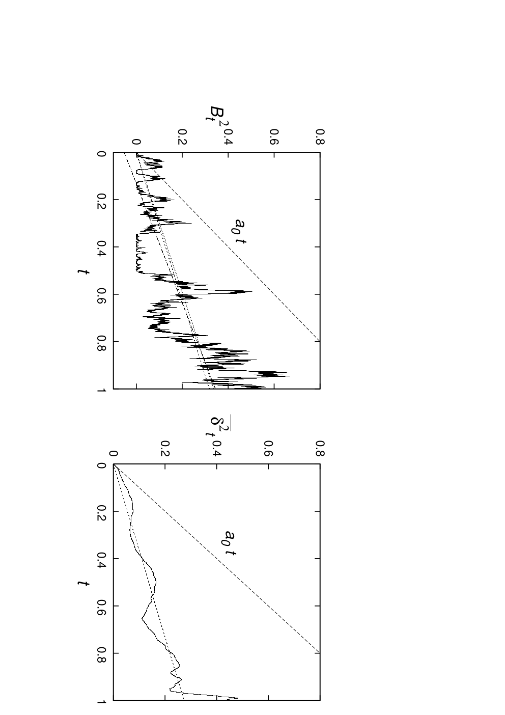
Another related method, often used in particle tracking experiments [6] and numerical studies [5], consists in least-squares fitting the time-averaged square displacement, . For a finite trajectory, this quantity is defined as
| (7) |
Due to the ergodicity of normal diffusion processes, at times short compared to 1 the above average coincides with the ensemble average [8], i.e., as . However, due to practical limitations, experimental trajectories often have a small number of positions and is analyzed for all (or a large fraction) of the available intervals , like in ref. [6]. Similarly, we do not restrict here to but fit over the whole time domain instead. As shown by the numerical example of Figure (1-right) for a random walk with positions, the expected small behavior of can be restricted to a very small interval compared to the total walk duration. Substituting by in Eq.(1) and adopting the linear fit, the new estimate simply reads:
| (8) |
Yet another fitting method consists in maximizing the unconditional probability of observing the whole trajectory , assuming that it is drawn from a Brownian process with mean-square displacement . Namely, the maximum likelihood estimate (MLE), denoted as , is the value of that maximizes the likelihood of , defined as:
| (9) |
where is the probability density of the Brownian process with constant . By equating to zero, one obtains
| (10) |
The estimates given by the four methods above are represented in an example, see Figure (1). The numerical values are comparable but can differ significantly from unity.
3 Numerical results
The numerical distributions of the random variables , , and are displayed in Figure (2).
The distributions are highly asymmetric and peaked near , far from the average value . The most probable is a small positive number in each case, see Table 1. Although estimates of can be sometimes observed, the median of the distribution is lower than . Namely, the probability of measuring a diffusion constant lower that the correct value is not 1/2, but close to 2/3 in all four cases. The probability of measuring a negative is not zero in the affine method (as already noticed in ref. [6]) but close to 0.175. Table 1 summarizes the main properties of the distribution functions.
Importantly, and practically obey the same distribution (Figure (2-right)), which is somewhat unexpected as is a much smoother function than . Thanks to this similitude, the analytical study of the simpler functional (4), exposed in the next Section, brings many insights on the behavior of . Distributions similar to ours for were determined in ref. [6], both numerically from random walk simulations and experimentally using R-phycoerythrin proteins in mammalian cells.

| 1 | 1 | 1 | 1 | |
|---|---|---|---|---|
| most probable | 0.11 | 0.16 | 0.01 | |
| median | 0.54 | 0.56 | 0.66 | 0.42 |
| lower 5 | 0.086 | 0.12 | 0.17 | -0.20 |
| upper 5 | 3.43 | 3.33 | 2.97 | 4.08 |
| Prob | 0.683 | 0.681 | 0.668 | 0.683 |
Table 1: Main properties of the diffusion constant distributions.
4 Feynman-Kac formalism for the generating function
In general the estimated fit parameters discussed above (FIT1, 2 and 4) are quadratic functionals of Brownian motion and take the form
| (11) |
When on the quadratic functional is positive and its generating function of , is defined by
| (12) |
where is the probability density function of . In order to compute we consider the following average of a quadratic functional of Brownian motion:
| (13) |
where the expectation above is for a Brownian motion starting at at time . Clearly in this notation we have . We now write a Feynman-Kac type formula for by considering how the functional evolves in the the time interval . During this interval the Brownian motion moves from to , where is an infinitesimal Brownian increment such that and . Taking into account this evolution we can write to order
| (14) |
where the brackets on the right hand side denote the average over . The above may now be written as
| (15) |
Expanding to second order in and , taking the average over and equating the terms of and we obtain
| (16) |
which looks like a Schrödinger equation in a harmonic, time-dependent potential. The boundary condition for this equation is given by for all .
It is easy to see that the solution of equation (16) is given by
| (17) |
where
| (18) | |||||
| (19) |
with the boundary conditions and . Now we can eliminate the nonlinearity in the second equation by setting which gives
| (20) | |||||
| (21) |
with the boundary conditions and . In terms of these functions the Laplace transform is now given by . We now make a change of time variable writing
| (22) |
assuming for the moment that is positive. In terms of this new temporal variable equation (21) can now be written as
| (23) |
In the class of problems we study in this paper (see Eqs.(4), (5) and (10)) the form of is
| (24) |
with and two constants. From this we can choose to be
| (25) |
and equation (23) becomes
| (26) |
The general solution to this equation can be shown to be
| (27) |
where and are modified Bessel functions [30]. The coefficients and are determined from the boundary conditions and at . Solving for and and using standard identities for Bessel functions [30] we find that at
| (28) |
and thus
| (29) |
5 Asymptotic analysis for the probability density function
The general result equation (29) simplifies in the case where , i.e. when , which is the case for FIT1 (linear) and FIT4 (MLE). In this case the probability density function of the estimator of the diffusion coefficient has support on . We start by analyzing the behavior of at small .
We proceed by using the small argument expansion of for :
| (30) |
to obtain the exact result
| (31) |
The moments of can then be extracted using the series expansion for modified Bessel functions [30] which gives
| (32) |
Without loss of generality we set and find the first two moments of to be given by
| (33) | |||||
| (34) |
and thus
| (35) |
In FIT1 and FIT4, a single estimator for the diffusion constant has the form
| (36) |
with and , respectively, which gives
| (37) |
From this we see that the MLE estimate of the diffusion coefficient has a variance where as the simple linear fit has a larger variance . Of course these variances can be computed directly and the above analysis serves as a check on our formalism to compute the full probability density function.
An interesting comparison can be made with the estimator which uses just the final value of the mean squared displacement
| (38) |
here we find the variance
| (39) |
which is clearly bigger than all the integral estimators above. Before embarking on inversion of the generating function to obtain the probability density function , a simple check of our results is to numerically compute from our simulation data. In Figure (3) are shown the Laplace transforms obtained from both Eq.(31) [or (32)] and the numerical distributions , we see that the agreement is perfect.

The behavior of at small values (when it is always positive) can be extracted by examining the characteristic function, or equivalently the Laplace transform of the probability density function of . Using the large asymptotic expansion
| (40) |
and setting , we find for large :
| (41) |
The behavior of at small can now be extracted by noticing that the integral
| (42) |
is dominated by its value at small and thus can be evaluated by the saddle point method as
| (43) |
from which we deduce that for small
| (44) |
From this we obtain the probability density of [Eq.(36)] at small to be:
| (45) |
The distribution exhibits an essential singularity at , as expected from the general asymptotic result of Shi [15]. For the linear fit estimate (), Eq.(45) gives
| (46) |
with
| (47) |
and for the MLE ()
| (48) |
with
| (49) |
The expressions above compare well with the simulation results at small (Figure (2-left), inset). The distributions (46) and (48) actually present a maximum at and , respectively. Despite that the asymptotic results start to fail when becomes too large, these values are still in good agreement with the most probable values of Table 1. A more detailed comparison in the small regime is displayed in Figure (4), where obtained from the numerics is plotted as a function of , with and . The behaviors at large arguments are nearly indistinguishable from the exponential laws predicted by Eqs.(46) and (48).

In order to extract the behavior of the probability distribution for large we need to examine the singularities of the generating function for , in this regime
| (50) |
from the identity . This Bessel function of the first kind oscillates and has simple zeros, at these zeros diverges. Let us denote as the lowest positive zero of . When from below,
| (51) |
where from above. We now note that
| (52) |
for . Comparing Eqs.(51) and (52), one deduces from (50) the large behavior:
| (53) |
For the linear fit (, ), one finds and
| (54) |
whereas for the MLE (, ), and
| (55) |
These asymptotic expressions are compared with the numerical results in Figure (5-left).


The interpretation of this result is rather straight forward, if we consider a Gaussian random variable of mean zero and variance then the probability distribution is
| (56) |
Now defining we find that the the probability density function of is
| (57) |
which has the same functional form as equation (53). This means that for large values of the random variable has the same distribution as a squared Gaussian random variable. This is not surprising as the variable can be viewed as an infinite sum of Gaussian random variables. Note that the full probability density function for the end point estimator is given by (as )
| (58) |
and so the distribution of this simple estimator decays much more slowly that the two integral estimators discussed above.
In the case of the affine fit, FIT2, both the estimators and , defined in equations (5) and (6), can be negative as the respective functions change sign. The probability density function is thus two sided. When becomes imaginary in Eq.(28), this solution must be modified by substituting and by and , respectively [30]. In turn, when becomes imaginary, and are replaced by and , respectively. For large the probability density function can be obtained from the closest zero of from zero in the negative direction, denoted by , and the analysis above goes through to give
| (59) |
in the case . For the variable , one finds and As can become negative we also have zeros of for positive values of ; now if the first of these zeros from the origin is then the same analysis as above implies, for :
| (60) |
in the case . For , one obtains and These asymptotic results are tested in Figure (5-right) on the two sided distribution arising for both the coefficients and , showing very good agreement.
6 Conclusion
We have shown that a general class of statistical estimators that can be used to extract diffusion constants from the squared displacement of single Brownian trajectories are in fact quadratic functionals of Brownian motion. Numerically we have seen that such estimators have a tendency to yield values which are typically lower than the correct average value. In addition we have seen that the statistics of the estimated diffusion constants from these trajectories resemble closely those obtained from fitting the time averaged squared displacement , defined in equation (7), despite the fact that the resulting trajectory appears much more regular than an unaveraged Brownian squared displacement, as demonstrated in Figure (1-right). An interesting and outstanding problem would be to carry out our analysis for estimators of type . Such an extension is clearly desirable as it deals with a quantity more commonly used in single particle tracking experiments. However from a technical point of view the resulting path integrals, while being for quadratic functionals of Gaussian processes, are highly non-local in time and it is probable that their evaluation will require the introduction of new mathematical methods.
Our final analysis was only limited by the problem of carrying out a full Laplace inversion of the generating function to obtain the full probability density function. However we point out that the generating function is actually easy to estimate from numerical data for the purpose of comparison with our analytical results, as demonstrated in Figure (3). In addition the generating function can be inverted analytically in certain asymptotic regimes. When the estimator is always positive, and consequently for , the behavior of for small can be extracted. We find that it has an essential singularity at and a maximum value, this estimate of the maximum value is in good agreement for the most likely value of coming from the full probability density function. For positive estimators the large behavior of turns out to be that of a squared Gaussian random variable, reflecting that fact that the estimator itself is an infinite sum of Gaussian random variables. This remains true when the estimator can have negative values, i.e when can change sign. In this case the probability density function for is that of a Gaussian squared for large as is that of for large negative .
Finally new methods are being introduced into single particle trajectory analysis to estimate diffusion constants and exponents associated with anomalous diffusion, for instance methods based on the mean maximal excursion [31], and it would be interesting to examine the distributions associated with such estimators.
Acknowledgements: We would like to than Alain Comtet and Marc Mézard for useful discussions on the subject of this paper. DB would like to thank the Université de Toulouse (Paul Sabatier) for an invited Professor’s position during which this work was initiated. DSD acknowledges support from the Institut Universitaire de France.
References
References
- [1] Saxton M J and Jacobson K 1997 Annu. Rev. Biophys. Biomol. Struct. 26 373–99
- [2] Pederson T 2000 Nature Cell Biol. 2 E73–74
- [3] Dix J A and Verkman A S 2008 Annu. Rev. Biophys. 37 247–63
- [4] Golding I and Cox E C 2006 Phys. Rev. Lett. 96 098102
- [5] Saxton M J 1997 Biophys. J. 72 1744–53
- [6] Goulian M and Simon S M 2000 Biophys. J. 79 2188–98
- [7] Rebenshtok A and Barkai E 2007 Phys. Rev. Lett. 99 210601
- [8] He Y, Burov S , Metzler R and Barkai E 2008 Phys. Rev. Lett. 101 058101
- [9] Lubelski A, Sokolov I M and Klafter J 2008 Phys. Rev. Lett. 100 250602
- [10] Cameron R H and Martin W T 1945 Bull. Amer. Math. Soc. 51 73–90
- [11] Borodin A N 1984 J. Math. Sci. 27 3005–22
- [12] Donati-Martin C and Yor M 1993 Adv. Appl. Prob. 25 570–84
- [13] Chan T, Dean D S, Jansons K M and Rogers L C G 1994 Comm. Math. Phys. 160 239–57
- [14] Revuz D and Yor M 1999 Continuous Martingales and Brownian Motion (Berlin: Springer)
- [15] Shi Z 1999 Lower tails of quadratic functionals of symmetric stable processes, Preprint Université Paris 6
- [16] Feynman R P and Hibbs A R 1965 Quantum Mechanics and Path Integrals, (New York: McGraw-Hill)
- [17] Kleinert H 2006 Path integrals in quantum mechanics, statistics, polymer physics and financial markets (Singapore: World Scientific)
- [18] Khandekar D C and Lawande S V 1986 Phys. Rep. 137 115–229
- [19] Dean D S and Jansons K M 1995 J. Stat. Phys. 79 265–97
- [20] Dean D S and Horgan R R 2005 J. Phys.: Condens. Matter 17 3473–97
- [21] Parsegian V A 2006 Van der Waals Forces (Cambridge: Cambridge)
- [22] Dean D S and Horgan R R 2007 Phys. Rev. E. 76 041102
- [23] Dean D S, Horgan R R, Naji A and Podgornik R 2009 Phys. Rev. A 79 040101
- [24] Dean D S, Horgan R R, Naji A and Podgornik R 2010 Phys. Rev. E 81 051117
- [25] Attard P, Mitchell J, and Ninham B W 1998 J. Chem. Phys. 88 4987–96
- [26] Podgornik R and Zeks T 1998 J. Chem. Soc. Faraday Trans 2 84 611–31
- [27] Podgornik R 1990 J. Phys. A: Math. Gen. 23 275–84
- [28] Dean D S, Horgan R R, Naji A and Podgornik R 2009 J. Chem. Phys. 130 094504
- [29] Majumdar S N 2005 Curr. Sci. 89 2076–92
- [30] Abramowitz M and Stegun I R 1972 Handbook of Mathematical Functions (New York: Dover)
- [31] Tejedor V, Bénichou O, Voituriez R, Jungmann R, Simmel F, Selhuber-Unkel C, Oddershede L B and Metzler R 2010 Biophys. J. 98 1364–1372