UT-11-02
IPMU11-0003
NSF-KITP-11-028
High–Energy Photon–Hadron Scattering in Holographic QCD
Ryoichi Nishio1,2 and Taizan Watari2
1Department of Physics, University of Tokyo, Tokyo 113-0033, Japan
2Institute for the Physics and Mathematics of the Universe, University of Tokyo, Kashiwano-ha 5-1-5, 277-8583, Japan
This article provides an in-depth look at hadron high energy scattering by using gravity dual descriptions of strongly coupled gauge theories. Just like deeply inelastic scattering (DIS) and deeply virtual Compton scattering (DVCS) serve as clean experimental probes into non-perturbative internal structure of hadrons, elastic scattering amplitude of a hadron and a (virtual) “photon” in gravity dual can be exploited as a theoretical probe. Since the scattering amplitude at sufficiently high energy (small Bjorken ) is dominated by parton contributions ( Pomeron contributions) even in strong coupling regime, there is a chance to learn a lesson for generalized parton distribution (GPD) by using gravity dual models. We begin with refining derivation of Brower–Polchinski–Strassler–Tan (BPST) Pomeron kernel in gravity dual, paying particular attention to the role played by complex spin variable . The BPST Pomeron on warped spacetime consists of a Kaluza–Klein tower of 4D Pomerons with non-linear trajectories, and we clarify the relation between Pomeron couplings and Pomeron form factor. We emphasize that the saddle point value of the scattering amplitude in the complex -plane representation is a very important concept in understanding qualitative behavior of the scattering amplitude. The total Pomeron contribution to the scattering is decomposed into the saddle point contribution and at most a finite number of pole contributions, and when the pole contributions are absent (which we call saddle point phase), kinematical variable dependence of evolution and evolution parameters and in DIS and -slope parameter of DVCS in HERA experiment are all reproduced qualitatively in gravity dual. All of these observations shed a new light on modeling of GPD. Straightforward application of those results to other hadron high energy scattering is also discussed.
1 Introduction
Despite plenty of data of hadron scattering, from which various qualitative features have been extracted, it remains difficult to derive and understand those features from the first principle, QCD, formulated as a perturbation theory. Gauge/gravity duality, however, can be exploited to study non-perturbative aspects of “hadron” in strongly coupled gauge theories. Many papers along this line focus on static properties of hadrons, such as mass spectra and three point couplings, but nothing prevents us from using gravitational dual descriptions to study “hadron” scattering of strongly coupled gauge theories at arbitrary energy scale [1, 2, 3]. Hadron–hadron scattering [1], total cross sections of deep inelastic scattering (DIS) [2], form factors of various conserved currents [4, 5, 6], and saturation/unitarity [7, 8, 9, 10, 11, 12, 13, 14, 15, 16] are examples of non-perturbative observables that can be studied in gravitational dual, but potential power of gauge/gravity duality in hadron scattering is far from being fully exploited so far.
Although perturbative QCD can describe evolution of parton distribution functions (PDF) and generalized parton distributions (GPD), initial data of the evolution cannot be determined by perturbation theory. Such non-perturbative initial data for PDF can be obtained from DIS experiments (and have also been studied in gravitational dual models [2]; see [17] for a list of articles on DIS in gravitational dual), but GPD cannot be determined even from experimental data, without some theoretical modeling of non-perturbative physics. GPD describes parton distribution in the transverse directions [18, 19, 20, 21] and two parton correlation in a hadron in general [22, 23, 24, 25, 26, 27], and hence it is an interesting object on its own. In this article, we take this non-skewed GPD and more generally deeply virtual Compton scattering (DVCS) [22, 23, 24, 25, 26, 27] amplitude at small as examples of hadron scattering, and see that gravitational dual descriptions can determine how those non-perturbative scattering amplitudes depend on kinematical variables such as center-of-mass energy, momentum transfer, impact parameter and photon virtuality. Gauge/gravity dual also tells us how to think about various theoretical ideas that various models of GPD have been based on.
High energy behavior of elastic scattering amplitude of two hadrons is characterized by poles and their residues of its partial wave amplitude on the complex angular momentum -plane (e.g., [28, 29, 30]); the poles and residues depend on momentum transfer . The poles in the -plane have often been assumed to depend linearly in , which is supported by the spectrum of mesons and hadron scattering cross sections at least for finite range of momentum transfer . Given the fact that the earliest version of string theory was born out of efforts to describe hadron scattering, it is not surprising that some successful aspects of classical Regge theory are preserved in gravity dual, string theory on a warped background. Notable aspects of string theory on a warped spacetime, however, include i) a single “Regge trajectory” of string theory on 10 dimensions gives rise to a Kaluza–Klein tower of infinite “Regge trajectories” on 4 dimensions, and ii) those trajectories do not remain linear for arbitrary negative [3]. The non-linear trajectories immediately result in non-Gaussian profile of GPD in the transverse directions (see section 4.2 of this article as well as [17]), although Gaussian profile of GPD is often assumed in phenomenological analysis. We will also describe how the residues of the Regge poles are determined by holographic set-up, and also explain how the Kaluza–Klein tower of Regge trajectories organizes itself to become a single contribution with a form factor in momentum transfer .
An extra energy scale —photon virtuality—is available in photon–hadron scattering, in addition to the center of mass energy and confinement scale . This extra parameter makes theoretical understanding of the non-perturbative amplitude interesting. The scattering amplitude is dominated by a contribution from a saddle point in the complex -plane, not from a pole, for sufficiently large . The saddle point value depends on kinematical variables such as , and . We find, by following this dependence of , instead of naively taking small limit or large limit, that observables characterizing scattering amplitude such as -evolution parameter , -evolution parameter and -slope parameter show qualitatively the same behavior in the strong coupling regime (gravity dual) as expected in perturbative QCD or observed in HERA DVCS experiment. As the saddle point value and the leading poles are both given by the kinematical variables of the scattering, crossover from the saddle-point phase to the leading pole phase may also be expected, when the photon virtuality decreases to a smaller value.11 1 A similar crossover behavior has already been observed in the real part to imaginary part ratio of the hadron–virtual “photon” scattering amplitude in gravity dual [11]. We will elaborate more also on this crossover behavior in section 4.3.
This article is organized as follows. Section 2 explains the set-up of gravitational dual for our calculation of photon–hadron scattering amplitude, while summarizing conventions and providing brief mini-reviews. Section 3 explains how the 2-body–to–2-body scattering amplitudes are given in the gravitational dual set-up, and presents an explicit form of Pomeron kernel; this section is largely a repetition of the contents of [3], but we believe that some small improvements are also made and subtleties clarified in derivation and final expression of the amplitudes and kernel. The photon–hadron scattering amplitude is discussed for zero skewedness in sections 4.1–4.3; section 4.1 explains momentum-transfer dependence of the imaginary part of the scattering amplitude, while its impact parameter dependence (i.e., transverse profile) is described in section 4.2. Section 4.3 is devoted to the real part of the amplitude. The interpretation of the scattering amplitude on a warped spacetime in Froissart–Gribov–Regge language on 4 dimensions is given in detail in section 4.1.3, while section 4.1.4 is devoted to the -slope parameter of the scattering amplitude. We will see in section 4.4 that GPD can be identified within the scattering amplitude even in the strong coupling regime, and discuss the form factor of GPD. In section 5, we address a question whether there is anything we can learn about GPD of the real world from the GPD calculation in the strong coupling regime. Section 6 briefly describes straightforward application of various results and observations in this article to other high-energy hadron scattering processes.
2 Model
Such gravitational backgrounds as [31, 32, 33, 34] are an ideal framework for holographic calculation of certain types of hadron interactions, as they have built-in confinement mechanism at IR, and allow renormalization group interpretation in terms of holographic radius. Those models have background geometry that are approximately with some compact 5-dimensional manifold , apart from the region near the IR boundary. The hard wall model [2] replaces these geometries with an background22 2 In our convention, . We use in labeling coordinates of ten dimensional spacetime, for the part, and for the coordinates of the 3+1 dimensional Minkowski spacetime. are dimensionless coordinates of , and is the metric of .
| (1) | ||||
| (2) |
An IR boundary is introduced at and boundary conditions on various fields are set by hand instead. The dilaton vev is simply assumed to be constant, . Such a background is not obtained as a stable solution to the Type IIB string theory, but Type IIB string calculations on such a background (while ignoring NS–NS tadpoles) are expected to maintain qualitative aspects of certain hadronic processes in the original holographic models. We use the hard wall model in the rest of this article, as it makes it possible to compute various physical quantities and study dynamics without consuming too much time.
Deeply virtual Compton scattering (DVCS) and double deeply virtual Compton scattering (DDVCS) are elastic scattering of a hadron and a (virtual) photon, , Figure 1, with the kinematics
| (3) |

As the target hadron, we use one of normalizable modes in a scalar degree of freedom on in the holographic set up. In particular, we use a scalar field originating from ten dimensional SUGRA fields upon Kaluza–Klein reduction on , just like in [35]. In case of reduction of dilaton, for example,
| (4) |
with a non-trivial harmonic function on , the target hadron corresponds to a glueball.33 3 To study DVCS and DDVCS of baryons, -branes should be used in the holographic set up, instead of a Kaluza–Klein mode of Type IIB SUGRA fields. We hope that there is still something to learn in an easier study with a scalar glueball target.
The holographic wavefunction of the target hadron is obtained by solving equation of motion derived from an effective action of the scalar field on . The bilinear part is
| (5) |
where
| (6) |
and a dimensionless constant44 4 It is defined as follows: (7) of order unity and a mass parameter depend on the choice of . When a Dirichlet condition55 5 Qualitative aspects of our results will not change, when a Neumann boundary condition is imposed, instead. is imposed on at the IR boundary , the wavefunction66 6 The wavefunction satisfies , so that the hadron field in has a canonical kinetic term upon dimensional reduction to 3+1 dimensions. of a hadron (corresponding to the -th normalizable mode) with incoming momentum is given by
| (8) |
where is the Bessel function, the -th zero point of , and . Mass of the hadron is given by
| (9) |
We will not specify the excitation level of the target hadron , as we will pay attention only to qualitative aspects of DVCS / DDVCS amplitudes, not to numerical details that depend on the excitation level .
As the (virtual) photon probe of DVCS / DDVCS amplitudes, we gauge an -symmetry associated with , and use it as a probe, just like in [2]. The type IIB metric field on 10 dimensions become a massless vector field on through
| (10) |
where is a Killing vector of , and . The kinetic term of the effective action of on is given by
| (11) |
with dimensionless coefficients77 7 Arbitrary chosen normalization of the Killing vectors does not remain in , as we define it by (12) the generators ’s are chosen so that they satisfy the same commutation relation as the Killing vectors, , and the Cartan metric remain the same. In the case a non-Abelian subalgebra of the Killing vectors of is gauged, in the kinetic term above should be understood as using the generators we explained above. and . The non-normalizable wavefunction of the vector field for the “photon probe” with incoming spacelike momentum is given by
| (13) | |||||
| (14) |
where is a dimensionless constant of order unity. , and is the polarization within the four dimensions. For sufficiently spacelike much larger than , the second terms and are negligible in (13, 14), but the full expression needs to be used for the final state on-shell photon in the DVCS.
The elastic scattering amplitude of a hadron and a (virtual) photon probe is calculated in holographic model by using the world-sheet non-linear sigma model with the background metric(1, 2) and inserting vertex operators whose Born–Oppenheimer approximation [36, 37] are specified by the wavefunctions (4, 8) and (10, 13, 14) [3]. The Compton tensor88 8 In the real world QCD with QED probe, where only fermion partons are charged under the probe, (15) is defined by removing polarization vectors,
| (16) |
and the goal of this article is to determine five independent structure functions99 9 Leading order perturbative QCD result in terms of non-perturbative GPD is found in [38] in the case of a scalar target hadron, and in [39] in the case of a fermion target hadron. See also [40, 41]. (e.g., [42]) in
| (17) |
The last term with the coefficient function should vanish for a scalar target hadron in a parity-invariant theory. Here, we introduced a convenient notation
| (18) |
Those structure functions, , should be expressed in terms of Lorentz invariant kinematical variables and , where
| (19) |
| (20) |
just as in standard literature in perturbative QCD. The parameter is assumed to be small
| (21) |
throughout this article. The two conditions on the kinematical variables (3) and (21) combined is sometimes referred to as generalized Bjorken regime. In this article, we focus on non-skewed DDVCS (). More general case () including DVCS () requires farther analysis. Holographic calculation of the DDVCS amplitude should reproduce the pure forward amplitude (whose imaginary part is the deeply inelastic scattering (DIS) amplitude studied in [2]) when the skewedness and momentum transfer are set zero; and .
For simplicity, we will study the sphere amplitude contribution to the four closed string external states. Although the sphere amplitude alone cannot discuss how the unitarity is maintained in the scattering, sphere amplitude is sufficient for large enough (or for not too large , for sufficiently large , or for sufficiently large impact parameter ). It is also possible to discuss with the sphere amplitude how the scattering approaches unitarity limit [11]. The pion cloud [43, 44, 45] contribution to the impact parameter dependent profile [46, 47], however, can be studied only in a more realistic holographic model containing pion [48, 49, 50, 51] by examining amplitude.
3 Pomeron Contribution to the Structure Functions
Holographic QCD has already been used to study DDVCS / DVCS amplitudes in the literature. Reference [42] calculated DDVCS / DVCS amplitudes for scalar target hadron (a set-up that we explained in the previous section), with a single supergravity field in the -channel resonance (see Figure 2). This contribution to the amplitude corresponds to the resonant contribution to the deeply inelastic scattering in the limit, and is known to be dominant in the large limit for moderately large ’t Hooft coupling and moderate [2].
 |
 | |
| (a) | (b) |
We can certainly learn the structure functions of DDCVS / DVCS processes in this way for the kinematical range mentioned above, but this sugra resonance contribution in the holographic calculation corresponds to the higher twist double trace operators of weakly coupled gauge theories, and does not tell us much about the non-perturbative input of GPDs.
The operators that are approximately twist-2 in perturbative gauge theories, on the other hand, have large corrections to the anomalous dimensions in strongly coupled regime (except the spin 2 operator). This “twist-2” contribution still dominates in the DIS amplitude for given at sufficiently small [2], and are naturally expected to be so in the off-forward DDVCS amplitude as well. In this article, we study this “twist-2” contribution in the small region by using holographic calculation, to get some hint on the non-perturbative input of the GPDs.
The “twist-2” operators of gauge theories correspond to string states in graviton trajectory in holographic descriptions [52, 3]. Contributions that involve such string states in the graviton trajectory to hadron scattering processes are called Pomeron amplitudes, and are known to be expressed as in (62) [2, 3, 11, 12]. In this section, we begin with refining the derivation of (62). Our derivation largely follows the ones in sections 2 and 3 of [3] and combine various improvements already made in [11, 12], but we believe that the following presentation also made a couple of small improvements. All of the following issues are closely related:
- a)
choice of integration contour in complex angular momentum plane,
- b)
validity of deformation of the integration contour,
- c)
origin of signature factor ,
- d)
absence of non-sense poles at negative integer angular momenta , and
- e)
the fact that the sphere amplitude of string theory is at best interpreted as a sum of -channel and -channel exchange of particles with various spins, not purely a sum of -channel amplitudes.
It will be made clear how we should think1010 10 By no means, we consider that the logical derivation in the following is the only possible one. about these issues a)–e) in writing down the Pomeron amplitude (62); interpretation provided in section 4.3 of this article is affected by the understanding on the issue e) we obtain here.
Another improvement is to replace , a derivative operator on often used in Pomeron propagator in the literature, by in (47) for complex angular momentum . The Pomeron wavefunction for spin is also introduced. Although this change does not leave a practical impact on the expression to be used as the Pomeron kernel (64), this extra conceptual clarification of the role played by complex angular momentum in the Pomeron kernel will enable us to provide clear theoretical understanding of the form factor associated with Pomeron-hadron-hadron coupling in section 4.1.
In section 3.2, we focus on DDVCS amplitude and find explicit expressions of Pomeron contributions to the five independent structure functions. It may be an option for busy and practical readers with some familiarity to [3, 11, 12] to skip section 3.1 for the first reading.
3.1 Pomeron Kernel from Sphere Amplitude
Reference [3] derives Pomeron kernel in its section 2 by modifying Virasoro–Schapiro scattering amplitude of closed string on 10-dimensional flat spacetime so that it is understood as an amplitude of scattering on a curved spacetime background (with small curvature ); we will combine it with the discussion in section 3 of [3] to fill a small gap in the process of modifying the scattering amplitude on flat 10-dimensions to that on the curved spacetime.
In flat 10-dimensional spacetime, the sphere level scattering amplitude of two NS–NS closed strings has a factorized form
| (22) |
where and are Mandelstam variables in 10-dimensions. The factor is a function of and , and independent of polarizations of the external strings;
| (23) |
The factor , on the other hand, is given by wavefunctions—momentum and polarization—of states involved in the scattering, whose explicit form is found in textbooks [53].1111 11 We follow [2], however, to use the factor that is times that of [53], and further includes delta function of momentum conservation; can be factored out from the factor [53], because we are interested only in the large small scattering, as in [2, 3]. Normalization of the factor is
| (24) |
for dilation–dilaton scattering, up to a constant of order unity. The factor for the case of our interest, dilaton–graviton scattering as a holographic model of DDVCS, is a little more complicated, because (dimensionless) polarizations of graviton external states are involved. We will first present the derivation of the scattering amplitude (62) and explicit expression of Pomeron kernel (64), using the case of dilaton–dilaton scattering. Polarization dependent statements are deferred to section 3.2.
We will study small DDVCS amplitude, with momentum transfer , (21), that is not necessarily smaller than the hadronic scale ; here, and are Mandelstam variables of 4D kinematics of DDVCS. This means, as we explain later, that we need to examine the Virasoro–Schapiro amplitude in the kinematical region , and , but not necessarily1212 12 This is a difference from the application to DIS in [2], where can be ignored. . Ignoring terms that are suppressed by or , one finds that
| (25) |
In this expression, contains -channel poles of strings. As long as1313 13 This is consistent with the well-known prescription in the quantum field theory, which defines the physical amplitude in the limit of . Moreover one can understand (26) as the average of in as in [2]. , in ,
| (26) |
As a result, one arrives at a well-known expression of the Regge behavior of the Virasoro–Schapiro amplitude on flat 10-dimensional spacetime:
| (27) |
There are a number of merits in seeing amplitudes in complex spin -plane in classical Regge theory [28, 29, 30], as well as in perturbative QCD [54, 29], and furthermore, the -plane description also has a couple of extra advantages in the present context. For one, we can clarify subtle points in how the derivation of Pomeron amplitude based on vertex operator OPE in section 3 of [3] is related to the somewhat heuristic modification of the flat spacetime amplitude in finding a scattering amplitude on a curved spacetime in section 2 of [3], as we explain shortly. Furthermore, we can find a clear guiding principle in the heuristic modification process of the scattering amplitude, although this process has not been crystal clear so far (in our eyes) in the literature.
Let us first see, with the -plane description, that can be decomposed into three pieces. First, note that the amplitude (27) is the same as
| (28) |
where , which is the trajectory of graviton, and the contour of integration in complex -plane is set as in Figure 3.
 |
 | |
| (a) | (b) |
Mathematically, one can add to the integrand a function of holomorphic at . In order to see the explicit relation with vertex operator OPE, we choose the following expression,
| (29) |
We will explain their relation soon, along with the meaning of , which is a real positive number. Secondly, suppose for now that
| (30) |
Then the integrand of (29) vanishes fast enough when goes to infinity while satisfying . It is, thus, possible to change the contour from to ; see Figure 3. The factor in the denominator is crucial in the convergence of integration at large real positive ; the condition (30) and the choice of are necessary for the convergence of integral along . Finally, let us split the integral along into two pieces, one with the factor in the integrand replaced by , and the other with the same factor replaced by . As a whole, is given by a sum of three pieces,
| (31) |
Physical meaning of the second term above will be clear. Replacing the -plane integral along by residues at the poles ,
| (32) |
which is regarded as -channel exchange of spin string on the graviton trajectory;1414 14 Although the factor of term in the summation seems to give rise to tachyon pole (i.e., ), the amplitude actually does not have such a tachyon pole. This is because a factor cancels the pole in term. the factor is understood as the propagator of a string with mass , and this contribution to the total amplitude is proportional to , as the dominant contribution to the factor in is proportional to .
Vertex-operator OPE in [3] in world-sheet calculation also yields the same expression as (32). Let us use -picture vertex operators
| (33) | |||||
| (34) |
for a massless incoming NS–NS string with and a massless outgoing NS–NS string with .
 |
 | |
| (a) | (b) |
The OPE of these two vertex operators includes the following series of operators
| (35) |
In the first line, we omitted terms which are less singular than in the limit.1515 15 The terms become those with the greatest power of , that is, . Less singular terms of OPE, whose coefficients are , have lower power of . This leading term in the OPE of string scattering in 10 dimensions becomes the leading term in small (large ) in the structure function in 4 dimensions in section 3.2. Leading terms of other structure functions in small , however, are determined in section 3.2 without using such an OPE on world sheet. Keeping only terms for simplicity, we obtain,
| (36) |
where1616 16 We adopt a convention of [53], where and vanish on physical states. Thus, and here corresponds to and in [3].
| (37) |
are weights of operator , and
| (38) |
The sphere amplitude is given by integrating over the entire complex plane. Only the terms remain, and
| (39) | |||||
| (40) | |||||
Because , we find that the contribution to this world-sheet amplitude has the structure of in (32).
Now in (28) has a clear meaning: the cut-off of integration of . The third term in (31), , corresponds to the contribution of the world-sheet amplitude above. Obviously the cut-off should be taken to infinity. Thus, the sphere amplitude using – OPE should be proportional to
| (41) |
There is no contradiction between (41) and (31); whenever
| (42) |
the contour can be chosen as a straight line from to for some . Now, it is easy to see that
| (43) |
because of the factor.1717 17 This also means that the -channel contribution has a finite limit. Moreover, because the total amplitude is also equal to (44) one can see that the -channel () contribution is equal to , at least mathematically. The -channel and -channel contributions are given by integral along and , respectively, and the total amplitude is given by . Although each piece of (31) is well-defined and such relations as (31, 41, 43) can be established only under the conditions (30, 42), the expression (28) is always well-defined, and it should be regarded as analytic continuation of the world-sheet amplitude1818 18 The same story is in between the Virasoro–Schapiro amplitude (23) and . (41) off the kinematical constraints (30, 42).
We have so far discussed Regge limit of closed string scattering amplitude in flat 10-dimensional spacetime, but our true interest is in scattering in a curved spacetime . The prescription of section 2 of [3] is to rewrite the factor in (24) by using wavefunctions of four external states in the scattering, and replacing and in by appropriate differential operators acting on the wavefunctions. We also follow this line of argument, while making a couple of improvements.
As the expression for becomes a little messy for dilaton–graviton scattering (holographic dual model of DDVCS amplitudes), we postpone working out the factor for this case until section 3.2. For an easier case, the factor for dilaton–dilaton scattering (holographic dual of elastic glueball scattering) becomes
| (45) |
where and are normalizable wavefunctions of the initial state hadrons, and is a dimensionless constant of order unity. in (24) is replaced by , including the warped metric.1919 19 Although also contains derivatives in and , such terms are ignored, because they are suppressed relatively by of order and are negligible in the high-energy scattering.
In order to obtain the factor for scattering in the curved spacetime , is replaced by the Minkowski part with the warped metric, just as above for the factor. As for in , on the other hand, one cannot drop such terms as or , unless [3]. Although it is not immediately obvious which derivative operators should be used in curved spacetime, we adopt a prescription to go to -plane description (29, 32, 40 41), first, and then replace in the spin partial wave by
| (46) |
where
| (47) | ||||
| (48) |
Since the factor in (32) is regarded as a propagator, the first two terms in (46) are the rank-2 differential operators appearing in the equation of motion of spin modes on the curved background.2020 20 and under the metric (2). In addition to this reasoning based on local field theory intuition, it is also possible to determine in direct calculation in worldsheet nonlinear sigma model. The last term is a mass correction; is a constant of order unity, and does not contain a derivative. The above prescription also can be applied to (28), because (28) is equivalent to (29).
Combining both the factors and , we obtain
| (49) | ||||
| (50) |
Note that all the derivatives in are placed on the right of all the -dependent factors and in the first line, and in the third line; simply acts on the wavefunctions . This is not asymmetric in and , because the derivative part of is Hermitian under the measure .
We will drop in the following; this is because on a compact space has non-positive discrete spectrum. Apart from the constant mode, whose eigenvalue of is zero, eigenvalues are negative and at least of order unity. Thus, at high-energy scattering,
| (51) |
a factor
| (52) |
in is always suppressed, unless is extremely small. The condition (51) corresponds to exponentially small in DIS/DDVCS,
| (53) |
which we will assume in later sections. The scattering amplitude now has an effective description in 5 dimensions,
| (54) |
where and are defined in (7).
The factor is non-local, and one can rewrite the factor as a diffusion kernel by inserting a complete system of the operator [3]. Eigenfunctions of ,
| (55) |
are given by
| (56) |
where is the modified Bessel function. Here, we imposed a Dirichlet boundary condition at IR in order to keep the expressions a little simpler, but essence will not change when a Neumann condition is imposed instead.2121 21 The reflection coefficient defined by (57) becomes under the Dirichlet boundary condition. It satisfies and for . (If both and are real valued, , although we do not use this property in this article.) When the Neumann boundary condition is imposed instead [3], defined as above also has all of these properties. For negative2222 22 We understand that is real positive for negative , that is, . In its analytic continuation to real positive through the upper half-plane in complex , then, . , the eigenfunctions for eigenvalues with form a complete system. Replacing by and using a relation
| (58) |
we find that
| (59) |
where , and
| (60) |
With a little more work, the expression above can be made completely symmetric for the two initial/final state hadrons; with a notation
| (61) |
one finally arrives at the expression we are familiar with in [3, 11, 12]:
| (62) |
where
| (63) |
for glueball–glueball elastic scattering. The Pomeron kernel becomes
| (64) |
Because (see (56)), in the kernel can be replaced by mathematically. We should remark that this expression (64) is valid only in zero-skewedness scattering.
It should be emphasized that we have in the Pomeron kernel, not that uses complex conjugate. This is a big difference, because the integrand in (64) can be regarded as a holomorphic function of (except some pole loci), and the kernel itself is expressed as a holomorphic integral in the spin–anomalous dimension plane;2323 23 This is quite common in perturbative QCD; e.g., [55, 56, 29, 3]. note that [3]. The kernel (64) is also holomorphic in the momentum transfer of hadron scattering, and we will exploit this nature in later sections.
The poles from correspond to the spin particle exchange, and contribute to the real part of the kernel. The so called nonsense poles of in Regge theory are canceled,2424 24 The factor also renders the total -channel exchange contribution finite, and makes the decomposition (31) possible, as we have already mentioned. and even become zeros in the -plane due to the factor in the -plane representation of the kernel. The absence of nonsense poles can easily be traced back to the Virasoro–Schapiro amplitude (23) and its Regge limit (27). One can also trace the origin of factor in the argument of vertex operator OPE; see (36).
The remaining singularity in the -plane comes from . vanishes at [3], because massless graviton does not receive mass correction even in curved spacetime (put another way, energy momentum tensor has vanishing anomalous dimension). is a function of , and hence the zero locus of the denominator determines the relation between and . The contour of integration is around this (-dependent) pole, and after integration, this pole locus determines the large (high energy) behavior of the scattering amplitude.
The pole locus in the -plane is given approximately by
| (65) |
for , and hence for . For , and hence for , one can still find the pole locus recursively [13]:
| (66) |
This means that the pole locus is shifted from due to the correction, not by an amount as large as the leading term, but by of order . The corrections are just as important as the term in . Finally, for , and hence for , it even becomes impossible to try to find the pole locus recursively. It is also known that for , - relation changes drastically [52]. To recap, the high-energy behavior of the Pomeron kernel is described fairly well by for , but the exponent begins to deviate from quadratic in , when becomes comparable to . This is equivalent to
| (67) |
loosely speaking, that is when , ‘‘the Kaluza--Klein momentum of Pomeron in the holographic radius direction’’ becomes comparable to the string scale.2525 25 Another condition , which was used already at (25), is satisfied for smaller than or saturating (67); this is because remains , while we consider .
3.2 Extracting Structure Functions of DDVCS Amplitudes
Although the Pomeron kernel (64) is universal for all the hadron scattering processes at high energy (small ), the impact factors and should be chosen for individual processes. in (8, 63) can be used for elastic scattering of two scalar glueballs [3, 12]. Two independent structure functions of DIS cross section are also expressed as in (imaginary part of) (62), using (8, 63) for the target hadron impact factor ; the impact factors for virtual photon have also been determined for the two structure functions [2]. In the case of DDVCS amplitudes for a scalar target hadron, there are five independent structure functions, and we need to determine the impact factors for these individual structure functions.
As a holographic model of DDVCS scattering, we use graviton–dilaton scattering, as we have announced in section 2. In order to determine the impact factors for the DDVCS scattering, it is easiest to start from the known form of the factor in (22) for the graviton–dilaton scattering, and carry out the process corresponding to (45), the same strategy as in [2]. For DDVCS,
| (68) |
where is a constant of order unity; and should be understood as wavefunctions in (13, 14) except the plane wave part already taken into account in the four momentum conservation. For the for incoming virtual photon and for outgoing virtual photon, the wavefunction with and the one with should be used, respectively. We have kept only the terms where four momenta of graviton ’s and dilaton ’s are contracted in (68), because such terms dominate in high-energy scattering, as in [2]. and are made symmetric in in (68), because the polarization of the graviton propagator is symmetric. Inserting the Regge limit process-universal amplitude to the right of and , we find that
| (69) |
For DDVCS at exponentially small , (53), only the constant mode on contributes, and the expression above is reduced to an effective description on 4+1 dimensions, just like in (54, 62); is now replaced by .
We are now ready to read off the impact factors for the DDVCS amplitude. The impact factor for the target hadron is the same as in the elastic scattering of the target hadrons, and is the same as (63). The impact factor for the virtual photon is
| (70) |
It can be decomposed into the five structure functions of (17); the result is as follows:
| (71) | ||||||||
where we treated all of and to be much smaller than unity.2626 26 We have already assumed . Here,
| (72) |
with
| (73) | |||||
| (74) |
When one ignores terms that are suppressed by powers of , as we have done so far, the five structure functions are in fact given by only two contributions, and . Although the longitudinal and transverse polarization of photon in the incoming beam axis is different from those in the outgoing beam axis in the presence of non-zero momentum transfer, they become approximately the same in small angle (and hence in small ) scattering; the two beam axes are precisely the same in the limit. In this sense, and correspond to the amplitude of the virtual photons with “longitudinal” and “transverse” polarizations, respectively.
4 DDVCS Amplitude and GPD at Small in Gravity Dual
Now that concrete expressions are given to the (Pomeron contribution to the) structure functions of DDVCS amplitude (71, 72), with an explicit expression for the Pomeron kernel (64), let us evaluate the integrals to get physics out of them. The momentum transfer dependence2727 27 For very large momentum transfer in the QCD in the real world, however, perturbative QCD can be used to argue rough scaling behavior [57, 58, 59, 60, 61] of the DDVCS amplitude. of DDVCS amplitude at small momentum transfer is highly non-perturbative information, and this is where gauge/gravity dual can play an important role.
We will first focus on scattering amplitude (i.e., structure functions) in sections 4.1–4.3; the imaginary part of the amplitude is studied in sections 4.1 and 4.2, which sheds a light on non-perturbative form of the parton distribution in the transverse direction at small [21]. The real part of the amplitude is described in section 4.3. We will argue in section 4.4 that GPD can be defined as an inverse Mellin transformation of operator matrix element and is calculable even in gravity dual; the structure functions and the scattering amplitude as a whole are given in the convolution form involving GPD, just like in the QCD factorization formula.
It is useful in studying the DDVCS amplitude in the generalized Bjorken regime (3, 21) to write down the Pomeron kernel explicitly as follows. Carrying out integral around the pole , and using the explicit form of in (56) for the hard wall model, we obtain
| (75) |
| (76) |
Although both of the second lines of (75, 76) are equivalent to (77) when integrated over , those in (75, 76), which is not symmetric under the exchange of and , turn out to be a little more convenient than the symmetric expression (77) in evaluating the DDVCS amplitude;2828 28 The second line of (75, 76) can also be written as (77) The second term vanishes in the limit for fixed , and the Pomeron kernel on in [10] is reproduced; the limit of the Pomeron kernel in this article is different from the one in [10] only by a factor of , which becomes at . dominant contribution to the amplitudes comes from small region () because of the virtual photon wavefunctions localized toward UV boundary, and for such a small value of , the and terms in have quite different behavior as a function of . decreases rapidly toward positive , while toward negative . This is why the term has been turned into in (75, 76) by relabeling by .
4.1 Momentum Transfer Dependence of the Imaginary Part
The imaginary parts of the structure functions simply come from the imaginary parts of the integrals and (72), and their imaginary parts come from the imaginary part of in the Pomeron kernel. It must be straightforward to substitute the expression of the kernel above into (72) and evaluate them for kinematical variables of our interest; References [2, 11] (see the reference list of [17] for other articles) have done that for purely forward case , and we can just carry out a similar procedure of calculation for case as well. Before doing so, however, we find it worthwhile to write down the amplitude in the following form, which leads us to a better theoretical understanding of the amplitude.
Exploiting the kinematical constraint of the generalized Bjorken regime (21), we expand in the Pomeron kernel (76) in a power series and keep only the first term. Contributions to from the higher order terms are suppressed by powers of , because the integration over the holographic coordinate is dominated by the region . Ignoring the higher order terms is like dropping higher twist contributions in perturbative QCD. One can then see that the structure functions can be written as
| (78) |
where
| (79) | |||||
| (80) | |||||
We will see in section 4.1.3 that and correspond to OPE coefficient and matrix element of a “twist-2” spin operator2929 29 Because of the factor in the integrand of (80), the second line in (80) is normalized to be unity at UV boundary . A careful reader may notice that is assumed in the expression of (80). This assumption gives rise to no problem, since throughout this article we always estimate the integral (78) in the lower half -plane. .
The two factors and depend on kinematical variables and as follows:
| (81) |
where , and
| (82) |
is a constant of order unity that depends only on (when , so that ), while the dependence of the structure functions now remains only in a dimensionless factor whose definition can be read out from (80, 82). Therefore, the imaginary part of the structure functions are given by
| (83) |
4.1.1 Small momentum transfer:
Now let us evaluate the amplitudes (83), first, for the case with small momentum transfer . The purely forward amplitude (i.e., one for the DIS total cross section) is a part of this story. The integration can be evaluated by the saddle point method for exponentially small (53), just like in [11]. The factor has a non-zero finite (dimensionless and ) limit when , and is a slowly changing function of , unless . Thus, large dependence comes only from
| (84) |
in (83). The saddle point is determined by the kinematical variables3030 30 As we discussed around (66), the expression of the kernel (75) is valid for . Therefore, the kinematical variables are restricted within the following region: (85) and as in
| (86) |
and the amplitudes approximately become
| (87) |
This leading order expression of the saddle point approximation (87) can be improved by going to higher order; those terms would give rise to corrections that are suppressed relatively by powers of .
Ignoring all the factors of order unity and the Gaussian measure of the saddle point approximation, we find that the DDVCS amplitude for small momentum transfer is roughly of the form
| (88) |
These results can also be used for the DIS structure functions, with , and in the purely forward limit and .
To characterize the dependence and dependence of the DDVCS and DIS structure functions, let us introduce effective exponents, as often done in phenomenological analysis of structure functions.
| (89) |
From (88), we find that
| (90) |
Both and , and hence the and evolutions, are controlled by the saddle point value ; the saddle point value in (86) becomes large for large and decreases to zero for smaller .
The effective anomalous dimension for a given is positive for larger , and negative for smaller . This means that the (generalized) parton density decreases in evolution for larger and increases for smaller . For a given value of , turns from negative to positive as increases, and the (generalized) parton density at that value of begins to decrease; the parton splitting from to smaller becomes faster than the splitting from larger to . This is precisely the behavior expected in [2]. Note that the essence of seeing this expected behavior is in keeping the dependence of the saddle point value in small () and large () region, without naively taking limit. Parton picture still remains even in the strong coupling regime, although the parton contributions do not dominate in the DIS structure functions at moderate (), and the DGLAP evolution is very fast.
Similarly, for a fixed value of , becomes smaller than 1 for sufficiently small , rendering the -integration for moment convergent at [11].3131 31 One can also see the convergence directly, when the scattering amplitude is given by a complex -plane integral; the -integration for moments converge for all larger than the largest real part of the singularities in the -plane. For a given value of , increases for larger , implying that the (generalized) parton distributions rise more steeply toward for higher (see Figure 8 (a)). This observation has already been made in the purely forward case [17].
The discussion so far clearly shows the conceptual importance of the saddle point value of and hence of . The Pomeron amplitude corresponds to a sum of contributions from various states/operators of spin , and the sum can be expressed as a holomorphic integral in the complex -plane. Equivalently, this integral can also be expressed in the complex -plane, via the relation . The saddle point value reflects the “center of weight” of contributions from various . The whole amplitude approximately shows the -evolution and -evolution of “spin operator”, as clearly shown in (90). We will see later in this article that not just the and dependence of and in (90) but that of almost all the observable parameters (-slope parameter in section 4.1.4 and real part to imaginary part ratio in section 4.3) of the photon–hadron scattering amplitude are governed by the saddle point value .
The essence of the saddle point approximation is in the following expression
| (91) |
where we already assume that we are interested in the small and large region, and ignored various factors the are irrelevant to the determination of the saddle point. The anomalous dimension as a function of complex spin variable is [3]
| (92) |
in the hard wall model, where is the inverse function of . We obtain an approximation
| (93) |
The saddle point value of is a function3232 32 A little more careful discussion should be given in non-conformal theories. It will not be difficult, however, to incorporate the running coupling effect within weakly coupled gauge theories or separately within gravity dual descriptions. of , just like in (86) and in (93). The saddle point approximation at the leading order ignores terms that are suppressed by , but keeps full dependence at all order. Higher order corrections in the saddle point approximation take account of suppressed corrections.
One will notice that this argument does not rely on detailed form of the anomalous dimension very much. Indeed, exactly the same line of argument has been used in perturbative QCD for the study of behavior of PDF in the small and large region [54]. The anomalous dimensions of the twist-2 series of operators in weak coupling gauge theories (with some variations in the approximation scheme (e.g., double leading log approximation (DLLA))) are not the same as those in gravity dual models such as (92), but they can be continuously deformed from one to the other by changing the value of the ’t Hooft coupling [3]. Discussion so far makes it clear i) that contribution associated with the “twist-2” series of operators (parton contribution) does exist in the weak coupling and strong coupling regimes alike, ii) that the kinematical variable dependence of the parton contribution in the small and large region can be captured by the saddle point approximation (91, 93), and iii) that the evolution of the parton contribution remains qualitatively the same in the both regimes, despite the difference in the anomalous dimensions. This similarity of the parton component of a hadron in the both regimes is an encouraging factor in trying to take advantage of gravity dual descriptions to study non-perturbative aspects of partons in a hadron of a confining gauge theory (like the real world QCD). We will elaborate more on this in section 5.
4.1.2 Large momentum transfer:
Let us now evaluate the holographic DDVCS amplitudes (83) for large momentum transfer, . In this case, the second term of the integrand in (80) is negligible for almost all the range of , and moreover, the range of integration is effectively limited by , because the modified Bessel function falls off exponentially for . In the region, , the wavefunction of hadron shows the power law behavior, . Hence, is approximately,
| (94) |
where is independent of , and is of order unity. Because the factor in (94) is a rapidly changing function of for , this factor has an impact on the saddle point value of integration in (83). The saddle point now depends on , as in
| (95) |
and the saddle point approximation of the DDVCS amplitudes at leading order is given by
| (96) |
Ignoring factors of order unity and the Gaussian measure of the saddle point approximation,3333 33 The effective exponents introduced in (89) are still given by and ; the saddle point value of is now given by (95). Thus, the discussion in p.4.1.1 holds true also for this case without modification.
| (97) | ||||
| (98) |
It is customary in perturbative QCD to describe the momentum transfer dependence of GPD in terms of a “form factor” defined by
| (99) |
Since the GPDs become PDFs for and , the form factor should be in that limit. This form factor takes account of finite size of hadrons, and is non-perturbative in nature. There is no way calculating the form factor in perturbative gauge theories,3434 34 In the approach of [57, 58, 59, 60, 61], power-law scaling in energy can be concluded for large region, but still non-perturbative wavefunctions of partons are required for quantitative results. and experimentally measurable form factors (such as the electromagnetic form factor) are sometimes used for theoretical modeling of GPD (though it should depend on ) and for fitting of DVCS experimental data. With the holographic set up, however, it can be calculated from first principle.
 |
 | |
| (a) | (b) |
Just one common form factor is necessary for all the structure functions3535 35 Here, we talk of form factors describing dependence in the structure functions, rather than the dependence of GPD. Characterization of GPD in strong coupling regime is given in section 4.4, where we will see that the form factor of structure functions (100) can also be taken as that of GPD in the sense of (99). , because the expressions (88, 98) are both not much different for and , at least for small we have assumed so far. Taking ratio of (87, 88, 98) to , we find that
| (100) |
The form factor largely shows power-law dependence on at large momentum transfer, and for sufficiently large momentum transfer,
| (101) |
the exponent of is approximately given by .
The Regge behavior in the Virasoro–Schapiro amplitude does not lead to exponential dependence on the momentum transfer of DDVCS processes, because this factor works as an exponential cut-off for contributions from Pomeron with large Kaluza–Klein momentum in the direction of holographic radius. Pomeron with small still contributes, but the Pomeron wavefunction cuts off the IR region of for spacelike momentum transfer [3]. This exponential cut-off and the power-law wavefunction (8) of the target hadron combined results in the power-law dependence of the form factor, as we have already seen in (94).3636 36 This mechanism is similar to the way the power-law dependence of DIS cross section was obtained for moderate [2], although the integration along the holographic radius was limited by the non-normalizable wavefunctions of virtual photons (73, 74) in the DIS case, not by the Pomeron wavefunction as in this case. Gravitational form factor—the moment of non-skewed GPD—also shows power-law dependence on the momentum transfer [4, 62, 63, 64, 65].
Note that this power-law dependence of the form factor is a generic consequence of asymptotically conformal theories, and is independent of details of IR geometry in holographic models. The power is determined by the conformal dimension of the bulk field the hadron belongs to. The power-law behavior in the UV conformal holographic models is due to the cost of squeezing the entire hadron into a size of . This power-law behavior in holographic picture, however, should not be taken as an explanation for the power-law behavior observed in the real world hadron–hadron elastic scattering data at large momentum transfer , because the holographic models assuming large ’t Hooft coupling even at high energy is not truly dual to the real world QCD. The power-law behavior expected from the naive power counting based on the number of valence partons [57, 58, 59, 60, 61] should be close to the truth of the power law in the region. Despite this difference, it is an encouraging fact that the form factor of holographic models generically matches on to something semi-realistic (power-law behavior) at large momentum transfer , rather than to something totally different. There is a long tradition of using a GPD form factor with a power-law behavior in at the region (e.g., [66, 67, 68]), and it might be possible to provide a better theoretical foundation to such form factors. See also section 5.
To learn more about the structure of the non-perturbative form factor (100) in the strong coupling regime, let us examine the kinematical variable dependence of the form factor (100) more carefully. First, the dependence and dependence are not completely factorized. Although the form factor gradually approaches to power-law in with a common power , it does so under -dependent condition (101). Even within the region (101), the coefficient of the power-law also depends on and ; we find that an effective energy scale in is given by
| (102) |
and in particular, decreases for small (large ). Note also that this form factor and properly take account of dependence, not just dependence at a fixed value of .
In the extremely small limit (for a given value of ), however, does not become arbitrarily small, but approaches a finite value, . In this limit, the form factor greatly simplifies, to become
| (103) |
from which and dependence has disappeared. This is when .
4.1.3 Regge theory revisited
Regge theory and the dual resonance model had a close relation in description of hadron scattering in late 1960’s–early 1970’s. Certainly the dual amplitude on 3+1 dimensions were not able to explain power-law behavior in the fixed angle high-energy scattering on one hand, and the theoretical consistency of string theory hinted a spacetime dimension higher than 3+1 on the other. But, string theory on a warped spacetime has resurrected as a theoretical framework of high energy scattering of hadrons in strongly coupled gauge theories [1, 2, 3]. When the scattering amplitudes of holographic QCD are seen as an amplitude of hadrons in four dimensions, some part of the Regge behavior of the scattering amplitude of strings in ten dimensions still seem to remain. The Pomeron trajectories predicted by holographic QCD are not linear, on the other hand, and the complex -plane description of hadron scattering amplitude of holographic QCD may be a little different from what one naively imagines from traditional Regge theory with some linear trajectories. The question is, then, how they are different.
Preceding literatures [3, 11, 12] have already made efforts in providing complex -plane description of the scattering amplitudes of holographic QCD. Our discussion in sections 4.1.1–4.1.2 already shows the importance of the saddle point value of the scattering amplitude in -plane in extracting kinematical variable dependence of the scattering amplitudes. It is thus worthwhile to take a moment in this section 4.1.3 and elaborate more on -plane description of the hadron scattering amplitudes in holographic QCD. It is known that i) holographic QCD gives rise to Kaluza–Klein towers of Pomeron trajectories, and that ii) they are not linear. From these properties, we will see in the following that scattering amplitudes are described better by treating those trajectories individually for some kinematical range, while they are better described by treating a Kaluza–Klein tower as a whole for some other kinematical regions. Such transitions are triggered by the location of the saddle point in the -plane relatively to other singularities of the amplitude.
Let us begin with studying behavior of the DDVCS amplitude, not just for physical region of plane, but for region including real positive . The integrand of (75) can be regarded as a holomorphic function of and . The denominator of the second term, , becomes zero if
| (104) |
and these zeros in the denominator can be regarded as poles in the -plane for a given kinematical variable . As we analytically continuate the integrand from real negative in the physical kinematical region to real positive through the upper-half complex plane of , the poles in the -plane move and some of them show up in the region with real positive ; see (104). We introduce a notation ; if , there are poles in the lower-half -plane. The positions of such poles satisfying (104) are denoted by . Thus, for , the integration contour in the -plane needs to be deformed as in Figure 6 (a), which can then be rearranged as in Figure 6 (b).
 |
 | |
| (a) | (b) |
Contributions from the poles can be written as3737 37 Although we obtained (105) by analytical continuation of the amplitude from into through the upper half plane, there is another derivation. In section 3.1, we derived the Pomeron kernel by inserting the complete system (58) into (54), but we implicitly assumed that . For , however, (58) is not a complete system, as the “Schrödinger equation” may have discrete spectrum as well [3]. Indeed, the wavefunctions (117) become the discrete spectrum of by replacing with and with , respectively. The pole contributions (105) come from the discrete spectrum part of the inserted complete system.
| (105) |
where
| (106) |
and
| (107) |
| (108) | |||||
| (109) |
Under the conditions that
| (110) |
(from which follows), , and a dependent mass parameter is defined by
| (111) |
The factor can also be defined similarly to (108, 109) by replacing by () in (73, 74). Because the wavefunction of photon depends on , it has dependence on . Explicitly, one can find , and
| (112) |
where is independent of .
The expression (105) is precisely in the form assumed in traditional Regge theory:
| (113) |
Traditional theory was only able to assume a linear form
| (114) |
for simplicity or from fit to experimental data, but holographic QCD predicts a trajectory (106); it is approximately linear for (but not too large ), but it is not unless . The residues satisfy factorization condition; they factorize into and holomorphically in . This factorization is necessary for unitarity of hadronic scattering processes in 3+1 dimensions, which is not guaranteed a priori in a theory that is not based on a local field theory on 3+1 dimensions [28, 69, 70].3838 38 Factorization predicts relations among differential cross sections: [30]. Scattering amplitudes of dual resonance model and superstring theory in 10-dimensions have the factorization property [71], and the factorization (107) in 4-dimensions is remnant of the factorization in string theory on higher dimensions.
We have so far dealt with the (analytic continuation of the) scattering amplitude , but closer connection to the classical Regge theory can be established by clarifying physical meaning of in (106) and of the factorized residues (107, 109). The Pomeron–hadron–hadron coupling (109) looks like an overlap integration of three wavefunctions; two of them are those of the target hadron, and the last one satisfies
| (115) |
For a special case as in (109), when , and are related by and , this means
| (116) |
which is the equation of motion for spin string state3939 39 The mass of the string will differ from one in the flat space. But we have shown in section 3.1 that the mass shift can be consistently neglected within our approximation. on the graviton trajectory in , when ; this momentum in the 3+1-dimensional Minkowski spacetime is on the mass shell in this wavefunction, when the IR boundary condition is satisfied. Therefore, describes the spin–mass relation of 4D hadrons corresponding to the -th Kaluza–Klein mode in the spin string state in the graviton trajectory; is the leading trajectory, and with become daughter trajectories [3]. Normalizable wavefunctions of all the 4D hadrons in the trajectory (110) are reproduced from a single wavefunction
| (117) |
defined for ; the wavefunction for is simply the special case of the one above. One might refer to (117) as a wavefunction of the -th Pomeron trajectory. The Pomeron–hadron–hadron coupling is given by an overlap integral of two ’s along with this wavefunction of the -th trajectory. That is,
| (118) |
When , on the other hand, all the poles in the lower half -plane have moved back to the upper half plane, and the scattering amplitude is given by a continuous integration of real axis. The integration in (83) can be converted into integration4040 40 The integration contour becomes the one in Figure 7 (a). through a change of variables , but there is no pole in this integration, unlike in the traditional form of Regge theory amplitude (113); the DDVCS amplitude (78, 83, 87) that we studied in sections 4.1.1–4.1.2 for do not seem to be based on the Pomeron pole exchange idea, at least apparently.4141 41 It should also be kept in mind that the subleading contribution comes from the exchange of the second Pomeron trajectory (the term in (105) for , which is power suppressed, . Corrections to (87, 96) on the other hand, are suppressed only by . If so, while the coefficient of the factor for , , can be characterized as hadron–hadron–[Pomeron ] three point coupling (118), how should we characterize the coefficient of the factor for , , in the absence of Pomeron exchange picture?
Field theory dual language is useful in characterizing the factors , and in (78–80). Let us define
| (119) |
for a parameter that has a dimension of [length]. Then one can see that the two factors and correspond to OPE coefficient of a “twist-2” spin operator renormalized at , and matrix element of the spin operator renormalized at [72, 73, 74]. To be more precise, we can define
| (120) | |||||
by pulling out from . It is easy to see that the short distance scale drops out from (120), and can be expressed only in terms of low-energy data and renormalization scale . Now one can see that
| (121) |
Therefore, is regarded as the coefficient of of the matrix element of the target hadron with insertion of a twist-2 spin operator (that is, spin form factor or reduced matrix element). is now defined for arbitrary in the expression above, not just for .
Using Kneser--Sommerfeld expansion of modified Bessel functions,4242 42 For and arbitrary complex numbers and , (122) This is regarded as the Green function on with an infrared cut-off, seen as a propagation of a 5D field (left hand side), or of a Kaluza–Klein tower of 4D fields (right hand side). one can see for arbitrary complex and that
| (123) |
The spin form factor to be used in describing the DDVCS amplitude for and the hadron–hadron–[Pomeron ] three point couplings are related as above. Such a relation between a form factor and three point couplings of Kaluza–Klein hadrons ,
| (124) |
has been known for conserved currents [4, 5, 6]. Here, (123) establishes such a relation simultaneously for arbitrary , not just for a given spin, and that makes it possible to “sum up” Pomeron exchange amplitudes labeled by the Kaluza–Klein excitation level .
* * *
Now we know that the amplitude is given (approximately) by Kaluza--Klein tower of Pomeron pole exchange4343 43 As we are talking about closed string amplitude, contributions from a single trajectory cannot be regarded as their -channel exchange; they can be regarded as a sum of -channel and -channel exchange, however. See the review material in section 3.1. for large positive (), while the entire amplitude as a whole is approximated by the saddle point method for large negative (). Since in the hard wall model is positive, the latter should be applied for all the physical region . Such subtle things, however, depend on details of infrared geometry of holographic models, and cannot be regarded as a robust prediction of holographic QCD.
Imagine, for example, a holographic model corresponding to an asymptotic free running coupling constant (e.g. [75]). With the curvature changing over the holographic radius, the entire spectrum of the Schrödinger equation becomes discrete [3].4444 44 Although we talk of “asymptotic free” running, it is safer to consider gravity dual models corresponding to gauge theories with asymptotic free running only up to some energy scale, above which they become strongly coupled conformal theories (e.g. [75]). In this case, although there are many bound states in the spectrum of the Schrödinger equation, the continuous spectrum still remains. Thus, the densely packed poles are still followed by a branch cut along the real axis in the small region. As long as one pays attention to a certain region in the -plane, rather than to formal difference in the literally large negative limit, the such models pass for “asymptotic free” gravity dual models. Whenever we refer to asymptotic free gravity dual models in this article, this must be understood. It is now more convenient to write the amplitude in complex -plane, rather than in -plane.
 |
 |
|
| (a) | (b) | |
 |
 |
 |
| (c) | (d) | (e) |
The branch cut at in the hard wall model is replaced by a densely packed poles along the real axis, and there is no special value like for some critical change in the spectrum. The spectrum may change for different values of , like in Figure 7 (c) and 7 (d, e), but they are not different qualitatively. Thus, there is nothing wrong a priori in choosing the integration contour as in (d) or (e), even for a given spectrum.
There exists a convenient choice of the contour in the -plane, however. That is to let the contour to pass the saddle point , and treat all the poles to the right of the saddle point (i.e., ) as isolated discrete contributions. All the rest are treated as if they formed a continuous spectrum as in the hard wall model. As we will see in the following, whether there are some poles remaining to the right of the saddle point (e.g., Figure 7 (b, d, e)) or not still works as a criterion for various physical transitions, independently of detailed difference in various holographic models.
The saddle point in the -plane is understood as a consequence of two competing effects in the DDVCS. One is the factor, which is large for large real . The coupling of spin string state with a virtual photon, on the other hand, behaves as , where is the anomalous dimension of the operator corresponding to the string state. This second factor is small for large real . These two factors combined, (91), forms a saddle point in the -plane for (meaning ); it is quite generic for holographic models with that the large behavior4545 45 We are not talking about as large as , however. of the anomalous dimension is . (We neglect here correction from the factor of power of .) Thus, in the right-hand side of the saddle point in the -plane, , the larger the real part of a pole, the larger the contribution of the pole is. Writing down the amplitude as a sum of these poles, starting from the one with the largest real part of to the ones with smaller , we obtain a finite term sum that gives a good approximation to the amplitude. Individual contributions from the poles in the left hand side of the saddle point , on the other hand, becomes larger and larger as the real part of of the poles become smaller. Thus, their sum does not make sense4646 46 In “asymptotic free” gravity dual models in the sense of footnote 44, the series of poles stop at a certain small value of , and a branch cut starts toward large negative . Thus, the contour can be chosen so that the amplitude is given by a sum of all the individual pole contributions and an integral around the branch cut. The sum is thus, formally, well-defined in this sense. It will be obvious, because of the discussion in the main text, however, that the resulting many-term summation contains large cancellation between the cut contribution and the pole contributions, and is not as practically useful an expression as what we described in the main text. ; all contribution in the left hand side should be treated as an integration on a contour as in Figure 7 (d). All of these contributions combined can be evaluated by the saddle point method, as we have presented by using the hard wall model, and their contribution is
| (125) |
This contribution is even smaller than the one from a pole whose real part is even slightly larger than . This is why it is convenient to take the contour in -plane so that it passes the saddle point as shown in Figure 7 (d).
Then we can understand that there is a transition depending on whether the saddle point value has a larger real part than that of the leading singularity (one in the -plane with the largest real part), . It is easy to see this in (which we have already discussed in section 4.1.1).
| (126) |
where the transition is induced (assuming that is a decreasing function of along the real axis) at
| (127) |
Schematically, it behaves as in Figure 8 (a).
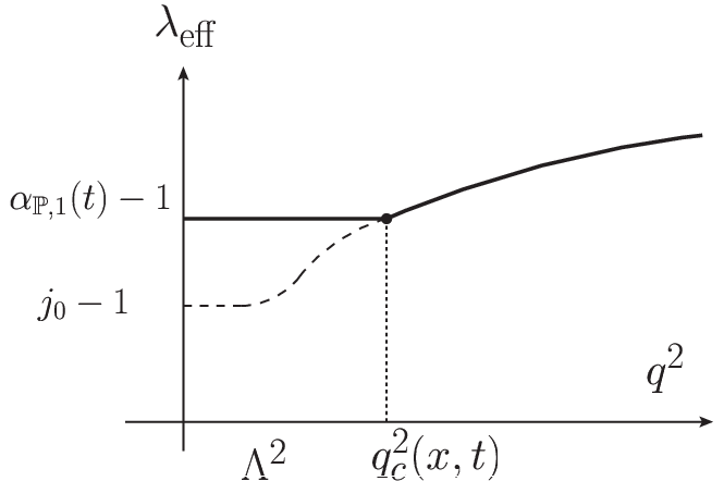 |
 | |
| (a) | (b) |
In the following, we will refer to the two phases4747 47 The KK-sum Spin-sum phase (saddle point phase) is divided into two phases, when the real part of the scattering amplitude is studied. One of them is still called KK-sum Spin-sum phase (saddle point phase), and the other as KK-sum low-spin phase (spin-2 phase). See [11] and section 4.3 of this article. as
- •
Low-KK Spin-sum phase or Leading pole phase (leading singularity phase), where the leading singularity has a larger real part than the saddle point, and
- •
KK-sum Spin-sum phase or Saddle point phase, where the saddle point value is larger than the real part of the leading singularity in the -plane.
It is intuitively obvious in gravity dual descriptions that the saddle point phase is realized (and such observables as and are controlled by the saddle point value ) for larger , not in the other way around; the holographic wavefunction of photon with larger virtuality makes the photon-[spin- string] couplings weaker, and the couplings for larger spin states are affected more severely than those for smaller spin states, because of the stronger power-law behavior of the holographic wavefunctions of the higher spin states. See (79) and definition of . The factor comes from there, and consequently, the saddle point value shifts to the right in the -plane to enter into the saddle point phase. See Figure 9.
In fact, the transition between the two phases is not a singular phase transition but a crossover, unless we literally take a small limit. As long as remains finite, the saddle point approximation is never exact, and the notion of the saddle point itself should be accompanied by a width proportional to . Although we defined the two phases by simply comparing the real part of the leading singularity and the saddle point , we should also keep in mind that the and higher Kaluza–Klein contributions give rise to finite corrections (for finite ) to the leading pole contribution in the leading pole phase; the corrections (and cancellation) may be sizable for negative and finite . For those reasons, the transition between the two phases can be a singular genuine phase transition only in the limit.

Phases are determined by kinematical variables , and kinematical variable dependence of all the observables, not just , will be different for different phases. Real part to imaginary part ratio of the scattering amplitude, which we study in section 4.3, is an example. Note also that the saddle point value depends on momentum transfer , not just on , and the leading Pomeron pole also depends on . Thus, the crossover should also be induced by the kinematical variable (at least somewhere in the -plane). In section 4.1.4, we study another observable, -slope parameter , and discuss its crossover behavior (like in Figure 8 (b)).
4.1.4 Slope parameter of the forward peak
We have so far focused on various features of the DDVCS amplitude that are robust and do not depend on detailed difference of holographic models. Individual holographic models, however, have full control over non-perturbative aspects of hadron physics, and more (possibly model dependent) information can be extracted. The expression (87), for example, tells us how to calculate full -dependence of the (imaginary) part of the DDVCS amplitude, not just for and the asymptotic region.
The slope parameter of forward peak (t-slope parameter) in the elastic scattering of two hadrons,
| (128) |
is an observable that characterizes the transition from region to region, and has been measured for and scattering at various energy scales (e.g., [30]). The slope parameter has also been measured in HERA experiment for scattering (DVCS) [76, 77, 78]. In this section 4.1.4, we will first use the hard wall model to derive an explicit prediction of the slope parameter in the photon–hadron scattering at vanishing skewedness (DDVCS process) for simplicity. Later on, we will discuss how much predictions on the slope parameter could be different for different holographic models, and discuss the possible crossover to be seen in the slope parameter (for some holographic models).
We define the slope parameter in non-skewed DDVCS by4848 48 We could define the slope parameter by the absolute value , not by the imaginary part as in (129). This choice, however, makes no difference as long as , and (the condition for the real part to be outside spin-2 phase); see section 4.3.1. This is because in this region the real-to-imaginary ratio of is not dependent on , (163). It is very likely that the most of the kinematical reach of DVCS measurement in HERA [76, 77, 78] is also in this region.
| (129) |
Let us first work out the prediction of the slope parameter in the saddle point phase, and then present the result in the leading pole phase later.
In the saddle point phase (KK-sum spin-sum phase), the factor in (87) does not contribute to the slope parameter, because the saddle point value does not depend on for . The slope parameter comes entirely from Pomeron–hadron form factor , which is regarded as a “spin form factor”. The Pomeron–hadron–hadron coupling behaving like a form factor is similar to the idea advocated in [79, 80], but the form factor turns out not to be precisely the same as the electromagnetic (spin 1) or gravitational (spin 2) one. There exists a notion of form factor that is holomorphic in spin , and the one with the saddle point value of is relevant for the DDVCS amplitude; the saddle point value is determined by as we have already seen in sections 4.1.1–4.1.2.
It is straightforward to calculate the slope parameter in the saddle point phase,
| (130) |
by using the explicit expression of the form factor4949 49 A grossly incomplete list of literatures on fixed spin form factor in holographic methods will include [4, 6, 81, 82, 83, 84, 85, 86, 62, 63, 64, 65]. (120). The result is shown in Figure 10.

The larger the spin (and hence ), the smaller the slope. At , the slope parameter is now the same as the “charge radius square” of the hadron under a “spin- probe”.
When the slope parameter is seen as a function of and , it changes only through the change in the saddle point value . Because
| (131) |
the slope parameter decreases for larger , and increases for larger in this saddle point phase prediction. It must be more sensitive to than to for small [], because of the denominators in (131). That is, we find the following qualitative prediction of the saddle point phase:5050 50 In this article, we assume the generalized Bjorken regime, (3, 21), exponentially small (53), and large ’t Hooft coupling, with an extra constraint (i.e., ).
| (132) |
There are three remarks here, before we move on to discuss predictions on the slope parameter from the leading pole phase. The first remark is on the size of the slope parameter of the forward peak. It is of order in this prediction of the saddle point phase, and is not tied to the slope of Pomeron trajectories; the asymptotic slope of the trajectories is of order (see (154)).
Secondly, let us discuss the momentum transfer dependence of the slope parameter within the saddle point phase. All the physical kinematical region is in the saddle point phase in the hard wall model, and the phase appears at least for sufficiently negative () for any other holographic models. Because of the power-law behavior of the form factor in UV conformal theories, the slope parameter behaves as for large . The slope parameter does not diverge toward (if all the range of is in the saddle point phase), however, and it approaches a finite plateau value of order instead. Whether there is a range of (in small ) where the amplitude shows exponential fall-off in is about the stability of the plateau value of for a finite range of , and about the plateau range and plateau value. This is a quantitative question whose answer depends on details of holographic models, and we do not discuss more about this question in this article.
Finally, it is important to note that the argument above on the and dependence of the slope parameter (132) can be applied to other observables of the DDVCS amplitudes, as long as they depend on and only through the saddle point value . Their and dependence are always opposite, and the dependence must be stronger at sufficiently small , because the saddle point has three properties:
| (133) |
This argument can be applied, for example, to and .
Let us now move on to the leading pole phase. Although all the physical kinematics is in the saddle point phase in the hard wall model, there may also be a range of the leading pole phase within the physical region in some holographic models, such as asymptotic conformal models with negative and asymptotic free models, as we have seen in section 4.1.3. In such holographic models, the crossover between the two phases may be observed in the slope parameter within the physical kinematic range . The slope parameter in the leading pole phase comes mainly from the factor
| (134) |
in the small and large region; the -dependence in the Pomeron coupling is now ignored. Thus, we have
| (135) |
For sufficiently small , this is of the order of
| (136) |
This is larger than the slope parameter in the saddle point phase, , in the small regime (53) we have been studying in this article. Thus, the crossover between the two different phases are induced schematically as in Figure 8 (b), where the large slope fall-off of the scattering amplitude in larger (more positive) breaks into smaller slope behavior in smaller (more negative) , when comes close to .
Even in asymptotic conformal theories with negative and in asymptotic free theories, where the leading pole phase may exist in the physical kinematical region , one always enters into the saddle point phase for sufficiently high ; this behavior is understandable just like in the case of .
It is an interesting question, at least from a theoretical perspective,5151 51 In reality, unitarity limit is reached and -suppressed contributions (that we ignored throughout in this article) also become important at sufficiently high energy. Such high energy region is described as phase IV in figure 9. and also from the context of fitting experimental data, whether such a crossover should be expected within the physical kinematical range . The answer is “no” in the hard wall model. But, the answer depends on infrared geometry of holographic models, and a robust conclusion cannot be drawn only from the experience in the hard wall model. It is interesting to know the answer to this question in holographic models whose infrared geometry is fully faithful to the equation of motions of Type IIB string theory [87].
4.2 Impact Parameter Dependence of the Imaginary Part
One can take a Fourier transform of ’s with , to obtain distributions in the impact parameter space. Such distributions are interesting on their own, because they show transverse spacial distribution of longitudinal momenta in the target hadron [21]. Also, unitarization of high energy elastic scattering amplitude and DIS cross section needs to be discussed in the impact parameter space, because all the partial wave amplitudes, i.e., for any values of impact parameter, should be unitary (e.g. [30]). Although the impact parameter dependent amplitude of hadron–virtual photon elastic scattering has already been formulated in [3, 10, 11, 12, 17] in holographic calculations, we elaborate more on this in the following, and find a result (151–153) and the phase diagram in Figure 13, which certainly refines the results that are already found in the literature.
The impact parameter dependence, and hence the momentum transfer dependence, comes mainly from the Pomeron kernel. The profile from the Pomeron kernel is extended over the size of order , as we will also see explicitly later. Although the virtual photon wavefunction also have dependence through , this dependence is relevant to the transverse profile only in the short distance of order , so we neglect this contribution. Thus, the impact parameter dependence purely comes from the Pomeron kernel. Fourier transform of the kernel is
| (137) |
The confinement effects (finite effects) are crucial for the impact parameter profile at long distance, . The profile in hard wall model shows quite different behaviors from one in conformal theory (corresponding to ) [12]. Because we are interested in hadrons in confinement, we examine the explicit form of the Pomeron kernel including the second term of (76), in detail.
As we have already mentioned in section 3 and section 4.1, the integrand of the Pomeron kernel (64, 76)5252 52 The “imaginary” part means the imaginary part when both and are real. The “imaginary part” and “real part” of the kernel separately become holomorphic functions of complex valued . is holomorphic (except some singularities) not just in spin and anomalous dimension , but also in momentum transfer , except at poles in (104). Thus, one can rewrite the kernel for on the real negative axis as
| (138) |
using the function holomorphic in (except the poles) and an integration contour which goes around the non-positive real axis counterclockwise (Figure 11 (a)).
 |
 | |
| (a) | (b) |
Its impact parameter space representation becomes5353 53 The following relation is used: (139)
| (140) |
Because of the holomorphicity in the complex -plane, the contour can be deformed as in Figure 11 (b), picking residues at the -dependent poles in the -plane; we can do this, because the integrand (for given ) vanishes exponentially at . One can show that
| (141) |
The imaginary part [resp. real part] of is obtained by taking imaginary part [resp. real part] of , as the Fourier transform works separately for the imaginary part and real part in (137). The -th term corresponds to the -th term of (105).
Let us examine the profile of the imaginary parts of in the impact parameter space. We will focus on a region
| (142) |
where the series of contributions from Kaluza–Klein tower of Pomeron trajectories (141) converges quickly; since the real part of is of the same order or larger than the hadronic scale at least for moderate value of and , we can approximate
| (143) |
Therefore, in this region, (142), the amplitudes (141) are dominated by the leading (lowest Kaluza–Klein) Pomeron trajectory, , and the contributions from the higher Kaluza–Klein trajectories are suppressed by of order .
At small , (51, 53), the impact-parameter dependent Pomeron kernel can also be evaluated by the saddle point method. In addition to the and factors, another factor may also give rise to a large dependence in ; dominant contribution to scattering amplitudes come only from small region in DDVCS as well as in DIS, and hence . The saddle point is, therefore, determined by
| (144) |
Therefore, we find that
| (145) |
Note that the saddle point value in the numerator is determined by (144), while in the denominator by (86). The -dependent transverse profile of parton distribution5454 54 The impact parameter dependent Pomeron kernel can be used also to determine the phase shift of the scattering amplitude in the impact parameter space, [10]. The relation between them is . In section 4.3, where we discuss the real part of the scattering amplitude, we will study the -dependent phase shift, rather than -dependent . is given by .
The transverse profile above is not a simple function, especially because depends on , and through (144). In order to extract the qualitative feature of the profile, let us first consider situations where the saddle point value is much smaller or much larger than unity. Then the following expansion of the zeros of Bessel functions of order , , can be exploited in order to understand how the saddle point value is determined by , and through (144):
| (146) | ||||
| (147) |
with positive numbers and of order unity [88].5555 55 for large . The saddle point stays within , when
| (148) |
and the saddle point is
| (149) |
On the other hand, when either of the left hand sides of (148) is much larger than unity, the saddle point becomes and
| (150) |
Now it is easy to see the transverse profile for large satisfying ; this situation corresponds to where is positive, that is, PDF decreases in DGLAP evolution, as we saw in section 4.1.1.
| (151) |
The profile remains linear exponential in the impact parameter for smaller , until it turns into Gaussian for larger .
Let us now study the transverse profile for smaller satisfying instead. This condition on corresponds to , when the PDF still increases under the DGLAP evolution, . The saddle point value becomes large for large which violates the second condition of (148). In this case, by using (150), the transverse profile turns out to be Gaussian approximately:
| (152) |
In a range of smaller impact parameter where , however, the expression cannot be simpler than
| (153) |
The transverse profile in this range of impact parameter is approximately linear exponential in (c.f. [17]), with the mass parameter changing slowly in . This approximate linear exponential profile (153) smoothly turns into the Gaussian profile (152), because of the dependence of the saddle point . All of these results5656 56 Note that for , neither (151) nor (152) are reliable, as we have used the form of that is reliable only in . For such a large impact parameter, the saddle point value of is not within this range. Similarly, for , (151) cannot be trusted. are summarized in Figure 13 (a).
Regardless of whether is large (151) or small (152), the imaginary part of the (sphere level) DDVCS amplitude shows Gaussian profile for sufficiently large impact parameter . The Gaussian profile in the transverse direction has been used for phenomenological fit of GPD, and the holographic calculation above justifies the Gaussian ansatz at least for sufficiently large impact parameter.
This agreement between the holographic calculation and the conventional phenomenological ansatz is not an accident. The phenomenological Gaussian ansatz is a direct consequence of a linear trajectory (114) in the traditional Regge ansatz (e.g. [30]). Although the Pomeron trajectories (110) in holographic QCD are not linear at all, they become approximately linear at large and (but not too large [52]), because of (147);
| (154) |
Since the saddle point for large is determined by the large behavior (and hence by the large (and large ) behavior) of the Pomeron kernel, the asymptotically linear trajectory (154) gives rise to the same large- behavior (that is, Gaussian profile) as in the phenomenological ansatz with a linear trajectory. The width-square of the Gaussian profile should be given by using the asymptotic slope parameter of the Pomeron trajectory in (154):
| (155) |
The Pomeron trajectories in holographic QCD are far from being linear, however, except for the large – asymptotic region. As a result, the transverse profile may well be different from the Gaussian profile at smaller (the region where ). Indeed, in this region, the results (151, 153) show that the profile is not Gaussian, but approximately linear exponential in the hard wall model. Interestingly, the mass scale of linear exponential profile for small in (153), , depends on kinematical variables, and is different from mass eigenvalues of any 4D hadron states; this linear exponential profile is not associated with a -channel exchange of a single particle, but emerges after summing up all the stringy states with different spins in the -th Kaluza–Klein trajectory. The mass scale appearing in the small limit (for fixed and ) is smaller than any one of the mass eigenvalues of the stringy (and graviton) states in the trajectory, and the range is longer than a simple -channel exchange of a glueball.
Although the expressions (151–153) rely on the hard wall model, most of its qualitative aspects are expected be in common with other holographic models. The transition from (152, 153) to (151) for larger , for example, will be induced in various models. The saddle point is dragged to larger , and for a given value of , just like we discussed in section 4.1.3.
4.3 Real Part of the Amplitudes
The imaginary parts of the structure functions are related to the GPDs, whose Fourier transforms are interpreted as the distributions of partons in the transverse spacial directions. Although the real part of the (D)DVCS amplitude does not have such an interpretation, it still contributes to the DVCS cross section.
The large impact parameter behavior of the real part has been discussed in [12], and the behavior in the small region (but not as small as ) is covered by [17]. Overall normalization is found in [11]. The following discussion provides a clear description of how the small behavior of ([17]) smoothly turns into the large behavior of [12], as well as careful interpretation of the physics behind this phenomenon. This subject has, in fact, quite a long history (e.g., [69]), but we hope that the following presentation using the saddle point value as a key concept helps clarify things a little bit.
4.3.1 Momentum Transfer Dependence
It is convenient (and customary) to use a variable
| (156) |
in characterizing the real part of the amplitude, as we already know the behavior of the imaginary part. The value of at is often denoted by in elastic scattering of hadrons.5757 57 The real part to imaginary part ratio is often denoted by , but is reserved for skewedness in this article. The real part of the amplitude is obtained by simply taking the real part of in the Pomeron kernel (64). The ratio is simply given by
| (157) |
using the saddle point value in the hard wall model [11] for the entire range of physical momentum transfer . The – integration in the kernel can be evaluated by the saddle point method for small (53), unless is too large to satisfy
| (158) |
The expression for above remains valid in other holographic models, as long as is in the saddle point phase. is predicted in gravitational dual in general, because is closer to 2 than to 1 for [11, 12].
In holographic models other than the hard wall model, there may be a leading pole phase in the kinematical variable space . There, the ratio is given by the expression (157) with the saddle point value replaced by the leading Pomeron pole [30].
The relation (157) follows immediately from derivative analyticity relation [89], if is understood as , the effective exponent of of photon–hadron scattering; such things as -plane representation of the scattering amplitude5858 58 Dispersion relation (159) in the convolution form becomes a simple product form after Mellin transformation, . This is why the ratio is better described in the -plane language. or its saddle point value do not have to be invoked in deriving the ratio (157). But, we still find the expression interesting, in that not only and but also and are predicted here to depend on the kinematical variables through a single value . Furthermore, the limit of applicability of (157), the condition (158), is translated into , which is to say that the GPD at that increases in the DGLAP evolution. This observation is based simply on the -plane representation of the scattering amplitude and an assumption that the kinematical variables are in the saddle point phase, and thus, does not rely on details of the hard wall model.
The condition (158) is not satisfied, however, for sufficiently large ; that is when , and GPD/PDF decreases under the DGLAP evolution.
 |
 | |
| (a) | (b) |
In this case, the contour of integration should be taken as in Figure 12 (b), and the structure functions are expressed as a sum of contributions from () pole and a continuous integration whose contour passes through the saddle point. For even larger , the saddle point value may be as large as and as large as , and the structure functions are given by a sum of contributions from some finite number of poles and the one from the saddle point approximation. Using the Kneser–Sommerfeld expansion of Bessel functions, these pole contributions () can be written in the form
| (160) |
Therefore, they are interpreted as -channel exchange of the -th Kaluza–Klein mode of the spin state in the graviton trajectory [11]. The remaining continuous integration should then be regarded5959 59 In this article, we used the dilaton–graviton scattering as the gravity dual model of the DDVCS process. If a D-brane is used as the model of the target hadron (baryon), however, the scattering amplitude is not a sphere amplitude with four NS-NS vertex operator insertion. as the -channel exchange of states and all the sphere level contributions associated with states.
Let us first focus on the region. Then, with a simple argument like we had in section 4.1.3, one can see that the () pole contribution dominates, other poles give rise to subleading corrections, and the saddle point contribution is even smaller than them [11].
The real parts of the structure functions are well approximated by the saddle point contribution for small enough , but they are expressed as a sum of pole contributions and the saddle point contribution, when becomes large enough to satisfy , that is,
| (161) |
This transition associated with the change in is understood as follows; it is usually better to treat the Pomeron trajectory exchange as a whole, not as a sum of exchange of individual spin particles, because the amplitude of a spin particle exchange has an ever-increasing factor . Large virtuality of the photon and the photon wavefunction localized near the UV boundary, however, introduces ––[spin string] coupling suppressed by powers of , and the amplitudes of higher spin exchange are suppressed significantly. The transition means that, for large , the power suppression becomes more important than for higher spin stringy states propagating in the sphere amplitude, and the contributions from smaller , that is, etc. “stand out” from all the rest. That is the physical meaning of the transition observed in the rearrangement of the integration contour. Therefore, we refer to this phase as
- •
KK-sum Low-spin Phase or Spin-2 Phase, where the saddle point value is larger than 2 (which also means ).
The discussion so far can be extended to the region ; the discussion in section 4.1.3 can be applicable almost in its form, except that the factor in (91) needs to be replaced by for ; the saddle point is the one using (95) in the hard wall model. The spin pole contributions can also be evaluated explicitly; they are
| (162) |
For a given value of and (so that ), the real part of the structure functions scale as , because the pole contribution dominates. For sufficiently large momentum transfer (so that ), however, the real part is better described by the saddle point contribution alone, and the real part shows the same scaling behavior in as the imaginary part of the structure functions. Therefore, the real part to imaginary part ratio is given by
| (163) |
For a given value of and , the ratio in the small limit is eventually given by (157) or possibly by the one with replaced by .
4.3.2 Impact Parameter Dependence
Although the impact parameter space description of the real part does not have such an interpretation as transverse distribution of partons, it still is important in discussing how the unitarity limit is reached in scattering. Since the unitarity limit is not achieved in the Bjorken limit without an extremely small (and extremely large ), the following discussion may be only of academic interest, but we present the result anyway.
The phase shift in the impact parameter space is given by [10]
| (164) |
at the leading order in expansion (sphere-level); the unitarity limit of the photon–hadron scattering in a “partial wave” is indicated when for and [10, 11, 12]. The saddle point in integration in the Pomeron kernel is determined regardless of whether we are studying impact-parameter dependent structure functions or phase shift; for , where only the Pomeron trajectory of the lowest KK 4D hadrons is relevant, we find
| (165) |
as long as the saddle point is not too large, and . Here, both the imaginary (absorptive) part and real (diffractive) part are included. The phase shift above shows expected dependence on , and , because and .
When the saddle point becomes large, , and hence , the diffractive (real) part of the phase shift needs to be treated separately, as we have already seen in studying the momentum transfer dependence. In terms of kinematical variables, for the lowest Kaluza–Klein mode is equivalent to
| (166) |
For either large or large , the diffractive part is written as a sum of pole contribution and the saddle point contribution, possibly with some other finite number of pole contributions. The pole contribution is always the dominant one as long as , and behaves as
| (167) |
where is the mass eigenvalue of the lowest Kaluza–Klein mode of graviton in the warped throat. This impact parameter dependent profile (167) is also a (and ) limit of the real part of (165). All these results are shown schematically in the phase diagram in Figure 13.
 |
 | |
| (a) | (b) |
The total cross section can be estimated by using the the sphere-level phase shift at high energy, provided that the absolute value of phase shift is of order unity or larger within the critical radius characterized by . Thus, the asymptotic form of the total cross section becomes
| (168) |
as long as . For even smaller (larger ) with a given , however, and become larger, and the condition will eventually be violated. The asymptotic behavior of then turns into
| (169) |
The total cross section of two light hadrons can also be discussed in a similar way; it can be calculated by replacing with . Then, the asymptotic behavior of becomes
| (170) |
for . In the very large region (), it becomes the form which is already shown in [12];
| (171) |
4.4 Structure Functions and GPD
We have so far used holographic QCD to calculate the DDVCS amplitude and its gauge-invariant structure functions. While the scattering amplitude is all the necessary information in describing experimental data, a little more theoretical object GPD represents internal structure of hadrons more directly.6060 60 At least in weak coupling regime, GPD is also considered important, not just scattering amplitudes, also because GPD can be used to describe amplitudes of multiple different scattering processes. In this subsection, we will argue that GPD is a well-motivated notion separately from the scattering amplitude or structure functions even in strong coupling regime (in holographic QCD), and show how to extract GPD from holographic calculation.
In the real world QCD, where only fermion partons (quarks and anti-quarks) are charged under the external probe (photon) of DDVCS, quark GPD in a scalar hadron is defined by
| (172) |
Its Mellin moment for an even integer is
where is the matrix element of the spin (symmetrized traceless) twist-2 operator,
| (175) |
Here, . The quark–anti-quark GPD, , is regarded as the inverse Mellin transform of , a holomorphic function of which becomes for .
Since matrix elements of gauge-invariant local operators are well-defined notion even in gravitational dual descriptions, we characterize GPD in holographic calculation as the inverse Mellin transform of a holomorphic function of , , which becomes matrix element of “twist-2” spin operator for . We have already seen in section 4.1.3 that in (120) is a holomorphic function of which becomes of some “twist-2” spin operator for . Thus, we can define a GPD renormalized at as the inverse Mellin transform of ; dependence of GPD6161 61 Discussion in this article needs to be refined in order to study skewedness dependence. can be calculated by using holographic QCD:
| (176) |
The GPD obtained in this way satisfy the expected DGLAP evolution, as one can easily see from the dependence of in (120).
Obviously GPD can be estimated in completely the same method as we have done in earlier sections for the structure functions. For the saddle point phase,
| (177) |
Note that the saddle point value now depends on instead of . The form factor for GPD defined in (99) is the same as (100) obtained by simply taking the ratio of structure functions at arbitrary to the ones at . Therefore, all the discussion on the form factor at the end of section 4.1.2 can be read as statements on the form factor of GPD in the saddle point phase of strong coupling regime. Note that the dependent form factor (100) and the effective mass scale are compatible with the renormalization group evolution.6262 62 Such models of GPD as in [67] and in [68] introduce ansatz of dependent GPD profile at a given renormalization scale. The profile at other renormalization scale needs to be determined numerically by following the DGLAP evolution. For the leading pole phase,
| (178) |
This is almost the same as the structure functions at the leading pole phase (112).
Certainly one can calculate a “GPD” in holographic QCD, but it is not clear at this moment GPD of which parton it is. We adopted an asymptotically conformal () geometry for holographic calculation, which means that the theory has all the particle contents of some conformal gauge theory. The reduced matrix element obtained in holographic calculation must be that of some linear combination of “twist-2” spin- operators of gluons, fermions and scalars of the gauge theory. It must be possible, at least, to specify the linear combination that has the smallest anomalous dimension. Purely background may also be replaced by a more realistic background. One could think of a couple of ways to refine the physical meaning of GPD obtained in this way, and possibly to obtain more results, but all of such improvements are beyond the scope of this article.
Relation between the structure functions of the Compton tensor and GPD in the strongly coupled regime (holographic calculation) remains quite similar to the one in the weakly coupled regime. To see this, let us first remind ourselves of relation between them in the weak coupling regime. Contributions from matrix elements of quark / gaugino twist-2 operators to the Compton tensor are formally written in the form of operator product expansion as
| (179) |
in perturbative QCD, the OPE coefficient can be calculated order by order in QCD coupling . Gauge-invariant structure functions can be extracted from the expression above. At tree-level in expansion, for example, the quark–anti-quark contributions to (some of) the structure functions at are given by
| (180) |
Thus, the structure functions at tree level at are expressed in terms of -plane integrals (inverse Mellin transforms) as in
| (181) | |||||
| (182) | |||||
Since the non-skewed structure functions in the complex -plane representation are given by products of the signature factor , operator reduced matrix element (or its -derivative) and its OPE coefficient , the structure functions become convolution of the inverse Mellin transforms of those factors. The factors in (181) and (182) originate from the inverse Mellin transform of the signature factor [90] here, but it also arises from the light-cone singularity of the fermion parton in direct calculation of the Compton tensor using Feynman diagrams [91].
In the holographic calculation of the structure functions of the DDVCS amplitude, we have seen that all the structure functions are given by , and are given by integration (78). The -integration becomes -plane integration, when the integration variable is changed through . The integrand is a product of the signature factor , reduced matrix element of some “twist-2” spin operator and a remaining -dependent factor, which is to be interpreted as the OPE coefficient and . Therefore, the structure functions of DDVCS amplitude are given even in the strong coupling regime by a convolution of a “propagator” , GPD (inverse Mellin transform of ) and inverse Mellin transform of OPE coefficient, just like in the weak coupling regime. The OPE coefficients in the strongly coupled regime, however, are calculated through the vertex operator OPE on world sheet; the OPE coefficients may be improved order by order in expansion, rather than in expansion in perturbative QCD.
5 Implication for the Real World QCD
We have so far studied DDVCS and GPD by using holographic QCD. In this section, we discuss how much we can apply our results in gravity dual to the real world QCD. We should keep in mind that the hard wall model or other UV conformal holographic models are not equivalent to the real world QCD. Dual gauge theories of UV conformal gravity descriptions remain strongly coupled, even in UV scale, if the gravity descriptions are to be reliable. If one considers an asymptotic free holographic model, so that it matches on to the asymptotic free QCD of the real world, then such a gravity description will not be a useful framework in the UV region of the holographic radius. Although there is such a difference, and a big gap that is very difficult to fill, it is also worthwhile to keep in mind that there are several features in GPD and structure functions that are shared by gravity dual descriptions and the real world QCD / perturbative QCD.
Factorization theorem holds for (D)DVCS and leptoproduction of mesons in the real world QCD [92, 93]. The structure functions are given by a convolution of hard kernel and GPD as in (181, 182). The hard kernel is calculable in the perturbation of the gauge coupling, whereas the GPD is incalculable, and should be given as non-perturbative input. It would be nice if GPD profile can be determined by experimental data alone, but that is known not to be possible. Even in setting constraints on the profile by using data, GPD has to be modeled and parameterized, because observable scattering amplitudes involve convolution of GPD, not just pure GPD, and furthermore, depend on GPD only in the limited region of kinematical variables. It is thus inevitable to construct physically motivated model of GPD.
Modeling and parametrization of GPD has already grown into a large field, as one can see in review articles (e.g., [25, 26]). The simplest model imaginable assumes factorized form of GPD into PDF and a -dependent factor [94, 95],
| (183) |
and models that mimic small Regge behavior were also considered [96, 97, 98, 99]:
| (184) |
with some -dependent function . In order to implement basic theoretical requirements on GPD, such as skewedness-polynomiality and proper DGLAP evolution, however, it is more convenient to have a framework of parameterizing GPD where such requirements are implemented systematically. There are two such frameworks of systematic parametrization. The first one is double distribution [100, 101, 102] along with -term [103]; transformation form this parametrization to GPD (Radon transformation) and its inverse is known [104, 105, 106]. GPD models in this parametrization framework are found, for example, in [104, 107]. The alternative framework of systematic parametrization is the collinear factorization approach, which is also known as dual-parametrization. In this approach, models of GPD are constructed as an amplitude on the conformal moment space [108, 109, 110, 111, 112]; GPD is given by a transformation [111] that becomes inverse Mellin transformation of for zero-skewedness.
Lessons from gravity dual calculation of DDVCS amplitude and GPD can be passed on to the understanding of GPD of the real world best in the form of -plane representation, , that is, in the collinear factorization approach (dual parametrization). The transformation between the -plane representation and Bjorken representation is just a pure mathematical one, and does not rely on perturbation theory or even on existence of a calculable theoretical framework. The description of the (D)DVCS amplitude in -plane is also based on OPE, which once again does not rely on perturbation theory [2]. While there is no way calculating hadron matrix element in perturbation theory, or in lattice gauge theory for complex valued , various gravity dual models yield at least some results (if not truly faithful to the real-world QCD), as we have seen in earlier sections.
The -plane representation of the scattering amplitude and GPD also plays an essential role in characterizing the following three phases of the behavior of GPD and (D)DVCS amplitude:
- •
: leading pole phase (or leading singularity phase),
- •
: saddle point phase, where ,
- •
: spin-2 phase, where .
The three phases are also interpreted as Low-KK Spin-sum phase, KK-sum Spin-sum phase, and KK-sum Low-spin phase, respectively, from above to below. The distinction between the last two phases is absent in GPD or in imaginary part of the scattering amplitude (at leading order in expansion), and we simply refer to the last two phases as saddle point phase. Earlier sections of this article described such a phase structure by relying on gravity dual calculation, but the essence is in the relative position of the leading singularity, pole and the saddle point in the -plane representation, not so much on details of gravity dual descriptions. As we have studied in sections 4.1.1 and 4.1.3, the parton dynamics characterized by and and the phase structure Figure 9 in plane (fixed slice) in gravity dual are surprisingly similar (qualitatively) to the one we know in the real world QCD. This similarity is traced back to the fact that the saddle point is determined by (93) in perturbative QCD as well as in holographic QCD, and that the anomalous dimensions in both frameworks are also qualitatively similar [3]; especially the two properties
| (185) |
are shared for certain range of .
Most of kinematical regions explored in DIS experiments should be in the saddle point phase (including the spin-2 phase in DIS),6363 63 The leading singularity phase tends to be realized in smaller , lower and less negative , and might be found experimentally. It is difficult, though, to tell theoretically where the phase boundary is located in the variable space in a theory with running coupling constant. as is clear from the dependence of and in DIS [113].6464 64 It is not very clear in low region, however, whether increases for larger [114]. c.f. Figure 8 (a). The leading pole phase may be hidden there. Anomalous dimension in the weak coupling regime6565 65 There are various approximation schemes in perturbative QCD, such as DLLA, BFKL and double leading approximation. should be used, because of the value of (depending weakly on ) closer to 0 than to 1 [113]. The GPD, then, is approximated by the expression (177) for some form factor evaluated at . This suggests (if the skewedness dependence that we did not study in this article does not screw things up) that various parameters characterizing the DVCS differential cross section6666 66 This parametrization of DVCS cross section by (conventionally adopted in data analysis) corresponds to .
| (186) |
namely, and above, as well as the real part to imaginary part ratio and the -slope parameter , are all functions of the saddle point value . Because of the way the saddle point value is determined, (93), all the four parameters are more sensitive to than to or in small , for the reason that we have already seen in (133). All of , , and are increasing functions of , and hence they increase6767 67 The HERA measurements give for GeV2, for GeV2, for GeV2, for GeV2, and for GeV2 in ZEUS [115], and for GeV2, for GeV2, and for GeV2, in H1 [78]. for larger . They should decrease for larger or larger , but only weakly. Although it is not immediately clear whether the slope parameter increases or decreases for larger (and hence for larger ), yet we found by using the spin form factor in the gravity dual hard wall model (in section 4.1.4) that the slope parameter decreases for large , which is in nice agreement with the HERA measurements [76, 77, 78].6868 68 In the leading pole phase with an anomalous dimension in the weak coupling regime, the slope parameter of the (D)DVCS differential cross section increases for larger , and depends only weakly on ; is used in (135). This prediction does not fit very well with the HERA data [76, 77, 78]. In this article, we did not work out gravity dual prediction for the -slope parameter in the spin-2 pole phase, where . The contribution from the real part dominated by a tower of spin-2 glueball exchange should be important there.
It is also worthwhile to remind ourselves that GPD models in the collinear factorization approach (dual parametrization) in the saddle point phase are always compatible with the renormalization group evolution. In the approximate form (177), the renormalization scale dependence comes into the form factor through the saddle point value .
All of these phenomenological as well as theoretical successes of the GPD models (177) come directly from the nature of the saddle point phase, as we have already seen above. One more necessary ingredient is that the slope parameter
| (187) |
is a decreasing function of ; this property of the hard-wall model prediction was used in explaining the dependence of the -slope parameter. It is a blessing indeed that the various features of experimental data are attributed to such a small number of conditions. To our knowledge, the first model of GPD in this category was that of [116], which introduces an ansatz
| (188) |
and are parameters of the model. All possible holographic models will also have their own predictions of the reduced matrix element (spin form factor) , and hence successful models of GPD in this category are obtained from these models, as long as (187) is a decreasing function of .
A general lesson from gravity dual calculations of the spin form factor is that even the leading trajectory (containing graviton) in 5-dimensions (or in 10-dimensions) becomes a Kaluza--Klein tower of infinite Pomeron trajectories for hadron scattering in 4-dimensions.6969 69 On top of this tower of infinitely many Pomeron trajectories, gravity dual descriptions predict yet another tower structure of trajectories, because stringy states form a tower of daughter trajectories already in the 5D (or 10D) description. The form factor is given in the following form
| (189) |
where the -th term corresponds to the -th Kaluza–Klein excited Pomeron trajectory; is the –spin relation. After summing up all the contributions in a Kaluza–Klein tower (189), however, the form factor has a power-law dependence in . This property is understood simply by using Green function in warped 5-dimensions; details of the background geometry of gravity dual models are irrelevant. This power-law behavior at large nicely matches on to the power law behavior expected theoretically from naive quark power counting [57, 58, 59, 60, 61], albeit only at qualitative level.
It should be kept in mind, however, that gravity dual descriptions are not an ideal and flawless framework in calculating the form factor. Although a gravity dual model with a carefully chosen background may serve as a faithful dual to the QCD of the real world, it should work as a reliable framework of calculation only in the IR region of the holographic radius. The UV region of the geometry should correspond to the real world QCD in the weak coupling regime, and hence the curvature of the background should be too large for a reliable calculation. It will be nice if it is possible to make even a crude estimate of the error in gravity dual calculation of the form factor (e.g., the power-law behavior from UV conformal gravity dual models is dictated by the conformal dimension associated with the target hadron, whereas the power is determined by the number of valence partons in the (empirically successful) naive power counting rule), and to use perturbative QCD in some way or other in controlling or reducing the error.
Such a dream may not be totally unrealistic, because at least one can compare singularities in the -plane representation. Gravity dual models for asymptotic free running coupling (at least up to some high energy scale), e.g., [75], can be used to calculate the isolated poles of . It is just to solve a Schrödinger equation [3]. Poles in the large region are reliable, because the corresponding wavefunctions are localized in the IR region of the warped spacetime, but those with smaller are not. On the other hand, the BFKL theory can calculate a spectrum of its kernel. The spectrum is discrete, when the running coupling effect is taken into account, and the discrete spectrum is mapped into poles in the complex -plane [29]. The spectrum of the BFKL theory in large region, however, corresponds to wavefunctions that are dominantly in the small (gluon transverse momentum) region, where the coupling is large and perturbation in does not work well. Thus, the BFKL theory might be used in determining the -plane singularities of in a region (smaller ) where the results from gravity dual cannot be reliable.
In the calculation of the form factor, the spectrum of the Pomeron kernel (poles in the -plane) is not the only necessary information. We also need corresponding wavefunctions of the spectrum, which are to be multiplied by a hadron impact factor, and integrated over the holographic radius , if we are to use the language of gravity description. Based on the similarity between the factorization formula of perturbative QCD and the expression (62) of hadron scattering amplitudes in gravity dual, correspondence between the coordinate of the BFKL theory and the holographic radius has been suggested [117, 118, 3]. Thus, the integration (and integrand) over the coordinate in the UV region may be replaced by that of the BFKL theory over the coordinate, in a crude attempt at improving the form factor calculated entirely in gravity dual models. All of such attempts, however, are beyond the scope of this article.
6 Discussion
In this article, we used holographic QCD to study double deeply virtual Compton scattering (DDVCS) amplitude and generalized parton distribution (GPD). Analysis presented in this article, however, is restricted to the scattering amplitude with vanishing skewedness; in order to exploit holographic methods to study non-perturbative aspects of deeply virtual Compton scattering (DVCS), analysis in this article needs to be extended to cover the case with non-zero skewedness. This subject will be covered in a future publication [87].
We have presented in this article an improved conceptual understanding of Pomeron couplings and Pomeron form factor, and predicted phase transition (crossover, to be more precise) in DDVCS amplitude. Such results, however, are not just for DDVCS and DVCS, but are more general in nature; some of the statements in this article hold true for some other high energy scattering processes only with minor (and almost obvious) modifications. An obvious generalization is to relax the constraint that the final state hadron is the same as the initial state hadron ; (Figure 14 (a)).
 |
 |
| (a) | (b) |
When the final state hadron and the initial state hadron are different Kaluza–Klein modes of the same field in the 5D effective theory, Pomerons (with vacuum quantum number) can couple to the transition from to . One only needs to replace the impact factor by in writing down the amplitude. Scattering amplitude of vector meson production (Figure 14 (b)) and timelike Compton scattering (Figure 14 (a) where the final state photon has timelike virtuality) can also be obtained by simply replacing the final state photon wavefunction properly. Since all of those processes involve an initial state spacelike photon with large virtuality, the initial state photon wavefunction localized strongly toward UV region gives rise to much the same and dependence of the Pomeron contribution to those scattering amplitudes. All of those processes involve a hadron–hadron–Pomeron vertex (lower blobs in Figure 14 (a, b)), and the non-perturbative vertex (form factor) in those processes should be essentially the same as in DDVCS. When the saddle point of the complex -plane representation of the scattering amplitudes has a larger real part than all the singularities in the -plane, the form factor depends on various kinematical variables (such as and ) only through the saddle point value , and the form factor becomes that of “spin current”. The -slope parameter can also be calculated for these processes, but it will be obvious that the our argument in section 4.1.4 is so generic that its conclusion holds true for vector meson production and timelike Compton scattering as well. There is sort of universality in the Pomeron–hadron –hadron form factor (coupling), regardless of whether it is used for DDVCS, DVCS, time-like Compton scattering or vector meson production (Figure 14 (a, b)).
We have also seen in this article that the (Pomeron contribution to the) DDVCS amplitude shows three qualitatively different behaviors; the three phases are characterized by the position of the saddle point of the -plane representation of the amplitude, relatively to the leading singularity and pole of the signature factor, as summarized in section 5. The essence of this phase classification is shared also by DDVCS/DVCS with , vector meson production and timelike Compton scattering. Since all of these processes involve the kinematical variable , spacelike virtuality of the initial state photon, it is not surprising to see a crossover behavior in the differential cross sections of these processes.
Acknowledgments
It is our great pleasure to express cordial gratitude to Kazuki Itakura and Yoshitaka Hatta, who gave a series of introductory lectures on hadron high-energy scattering at Tsukuba U., ’08 and at Tokyo U., ’10, respectively. We also thank Leonid Frankfurt, Andrei Mihailov and Shigeki Sugimoto for useful comments, and Simeon Hellerman and Tsutomu Yanagida for encouragements. Part of this work was carried out during long term programs “Branes, Strings and Black Holes” at YITP, Kyoto, October, 2009 (TW), “Strings at the LHC and in the Early Universe” at KITP, Santa Barbara, April–May, 2010 (TW), “High Energy Strong Interactions 2010” at YITP, Kyoto, August, 2010 (RN, TW) and also during a stay at Caltech theory group of TW. This work is supported by JSPS Research Fellowships for Young Scientists (RN), by WPI Initiative, MEXT, Japan (RN, TW) and National Science Foundation under Grant No. PHY05-51164 (TW).
References
- [1] J. Polchinski and M. J. Strassler, “Hard scattering and gauge / string duality,” Phys. Rev. Lett. 88 (2002) 031601, arXiv:hep-th/0109174.
- [2] J. Polchinski and M. J. Strassler, “Deep Inelastic Scattering and Gauge/String Duality,” JHEP 0305: (2003) 012, hep-th/0209211.
- [3] R. C. Brower, J. Polchinski, M. J. Strassler, and C.-I. Tan, “The Pomeron and Gauge/String Duality,” JHEP 0712: (2007) 005, hep-th/0603115.
- [4] S. Hong, S. Yoon, and M. J. Strassler, “Quarkonium from the fifth dimension,” JHEP 04 (2004) 046, arXiv:hep-th/0312071.
- [5] S. Hong, S. Yoon, and M. J. Strassler, “On the couplings of vector mesons in AdS/QCD,” JHEP 04 (2006) 003, arXiv:hep-th/0409118.
- [6] S. Hong, S. Yoon, and M. J. Strassler, “On the couplings of the rho meson in AdS/QCD,” arXiv:hep-ph/0501197.
- [7] S. B. Giddings, “High energy QCD scattering, the shape of gravity on an IR brane, and the Froissart bound,” Phys. Rev. D67 (2003) 126001, arXiv:hep-th/0203004.
- [8] K. Kang and H. Nastase, “High energy QCD from Planckian scattering in AdS and the Froissart bound,” Phys. Rev. D72 (2005) 106003, arXiv:hep-th/0410173.
- [9] L. Alvarez-Gaume, C. Gomez, and M. A. Vazquez-Mozo, “Scaling Phenomena in Gravity from QCD,” Phys. Lett. B649 (2007) 478–482, arXiv:hep-th/0611312.
- [10] R. C. Brower, M. J. Strassler, and C.-I. Tan, “On the Eikonal Approximation in AdS Space,” JHEP 0903: (2009) 050, 0707.2408.
- [11] Y. Hatta, E. Iancu, and A. H. Mueller, “Deep inelastic scattering at strong coupling from gauge/string duality: the saturation line,” JHEP 0801: (2008) 026, 0710.2148.
- [12] R. C. Brower, M. J. Strassler, and C.-I. Tan, “On The Pomeron at Large ’t Hooft Coupling,” JHEP 0903: (2009) 092, 0710.4378.
- [13] L. Cornalba, “Eikonal Methods in AdS/CFT: Regge Theory and Multi-Reggeon Exchange,” arXiv:0710.5480 [hep-th].
- [14] L. Alvarez-Gaume, C. Gomez, A. Sabio Vera, A. Tavanfar, and M. A. Vazquez-Mozo, “Critical gravitational collapse: towards a holographic understanding of the Regge region,” Nucl.Phys. B806 (2009) 327–385, arXiv:0804.1464 [hep-th].
- [15] Y. V. Kovchegov, Z. Lu, and A. H. Rezaeian, “Comparing AdS/CFT Calculations to HERA F(2) Data,” Phys.Rev. D80 (2009) 074023, arXiv:0906.4197 [hep-ph].
- [16] Y. V. Kovchegov, “R-Current DIS on a Shock Wave: Beyond the Eikonal Approximation,” Phys.Rev. D82 (2010) 054011, arXiv:1005.0374 [hep-ph].
- [17] R. C. Brower, M. Djuric, I. Sarcevic, and C.-I. Tan, “String-Gauge Dual Description of Deep Inelastic Scattering at Small-,” arXiv:1007.2259 [hep-ph].
- [18] M. Burkardt, “Impact parameter dependent parton distributions and off forward parton distributions for zeta 0,” Phys.Rev. D62 (2000) 071503, arXiv:hep-ph/0005108 [hep-ph].
- [19] J. P. Ralston and B. Pire, “Femtophotography of protons to nuclei with deeply virtual Compton scattering,” Phys.Rev. D66 (2002) 111501, arXiv:hep-ph/0110075 [hep-ph].
- [20] M. Diehl, “Generalized parton distributions in impact parameter space,” Eur.Phys.J. C25 (2002) 223–232, arXiv:hep-ph/0205208 [hep-ph].
- [21] M. Burkardt, “Impact parameter space interpretation for generalized parton distributions,” Int. J. Mod. Phys. A18 (2003) 173–208, arXiv:hep-ph/0207047.
- [22] X.-D. Ji, “Off forward parton distributions,” J.Phys.G G24 (1998) 1181–1205, arXiv:hep-ph/9807358 [hep-ph].
- [23] A. Radyushkin, “Generalized parton distributions,” arXiv:hep-ph/0101225 [hep-ph]. To be published in the Boris Ioffe Festschrift ’At the Frontier of Particle Physics / Handbook of QCD’, edited by M. Shifman (World Scientific, Singapore, 2001).
- [24] K. Goeke, M. V. Polyakov, and M. Vanderhaeghen, “Hard Exclusive Reactions and the Structure of Hadrons,” Prog. Part. Nucl. Phys. 47 (2001) 401–515, arXiv:hep-ph/0106012.
- [25] M. Diehl, “Generalized Parton Distributions,” Phys.Rept. 388 (2003) 41–277, hep-ph/0307382.
- [26] A. V. Belitsky and A. V. Radyushkin, “Unraveling hadron structure with generalized parton distributions,” Phys. Rept. 418 (2005) 1–387, arXiv:hep-ph/0504030.
- [27] S. Boffi and B. Pasquini, “Generalized parton distributions and the structure of the nucleon,” Riv. Nuovo Cim. 30 (2007) 387, arXiv:0711.2625 [hep-ph].
- [28] P. Collins, An Introduction to Regge Theory and High Energy Physics. Cambridge Monographs on Mathematical Physics. Cambridge University Press, 1977.
- [29] J. R. Forshaw and D. A. Ross, Quantum chromodynamics and the pomeron, vol. 9 of Cambridge Lect. Notes in Phys. Cambridge Univ. Pr., 1997.
- [30] V. Barone and E. Predazzi, High-energy particle diffraction. Texts and Monographs in Physics. Springer, 2002.
- [31] J. Polchinski and M. J. Strassler, “The String Dual of a Confining Four-Dimensional Gauge Theory,” hep-th/0003136.
- [32] I. R. Klebanov and M. J. Strassler, “Supergravity and a confining gauge theory: Duality cascades and SB-resolution of naked singularities,” JHEP 08 (2000) 052, arXiv:hep-th/0007191.
- [33] J. M. Maldacena and C. Nunez, “Towards the large N limit of pure N=1 super Yang Mills,” Phys.Rev.Lett. 86 (2001) 588–591, hep-th/0008001.
- [34] A. Butti, M. Grana, R. Minasian, M. Petrini, and A. Zaffaroni, “The Baryonic branch of Klebanov-Strassler solution: A supersymmetric family of SU(3) structure backgrounds,” JHEP 0503 (2005) 069, arXiv:hep-th/0412187 [hep-th].
- [35] H. J. Kim, L. J. Romans, and P. van Nieuwenhuizen, “The Mass Spectrum of Chiral N=2 D=10 Supergravity on S**5,” Phys. Rev. D32 (1985) 389.
- [36] R. Rohm and E. Witten, “The Antisymmetric Tensor Field in Superstring Theory,” Ann. Phys. 170 (1986) 454.
- [37] J. Distler and B. R. Greene, “Aspects of (2,0) String Compactifications,” Nucl. Phys. B304 (1988) 1.
- [38] A. Radyushkin and C. Weiss, “DVCS amplitude at tree level: Transversality, twist - three, and factorization,” Phys.Rev. D63 (2001) 114012, arXiv:hep-ph/0010296 [hep-ph].
- [39] A. V. Belitsky and D. Mueller, “Twist- three effects in two photon processes,” Nucl.Phys. B589 (2000) 611–630, arXiv:hep-ph/0007031 [hep-ph].
- [40] L. Mankiewicz, G. Piller, E. Stein, M. Vanttinen, and T. Weigl, “NLO corrections to deeply virtual Compton scattering,” Phys.Lett. B425 (1998) 186–192, arXiv:hep-ph/9712251 [hep-ph].
- [41] A. V. Belitsky, D. Mueller, and A. Kirchner, “Theory of deeply virtual Compton scattering on the nucleon,” Nucl.Phys. B629 (2002) 323–392, arXiv:hep-ph/0112108 [hep-ph].
- [42] C. Marquet, C. Roiesnel, and S. Wallon, “Virtual Compton Scattering off a Spinless Target in AdS/QCD,” JHEP 04 (2010) 051, 1002.0566.
- [43] J. D. Sullivan, “One pion exchange and deep inelastic electron - nucleon scattering,” Phys. Rev. D5 (1972) 1732–1737.
- [44] S. Kumano, “Flavor asymmetry of anti-quark distributions in the nucleon,” Phys. Rept. 303 (1998) 183–257, arXiv:hep-ph/9702367.
- [45] G. T. Garvey and J.-C. Peng, “Flavor asymmetry of light quarks in the nucleon sea,” Prog. Part. Nucl. Phys. 47 (2001) 203–243, arXiv:nucl-ex/0109010.
- [46] M. Strikman and C. Weiss, “Chiral dynamics and partonic structure at large transverse distances,” Phys. Rev. D80 (2009) 114029, arXiv:0906.3267 [hep-ph].
- [47] M. Strikman and C. Weiss, “Quantifying the nucleon’s pion cloud with transverse charge densities,” Phys. Rev. C82 (2010) 042201, arXiv:1004.3535 [hep-ph].
- [48] T. Sakai and S. Sugimoto, “Low energy hadron physics in holographic QCD,” Prog. Theor. Phys. 113 (2005) 843–882, arXiv:hep-th/0412141.
- [49] T. Sakai and S. Sugimoto, “More on a holographic dual of QCD,” Prog. Theor. Phys. 114 (2005) 1083–1118, arXiv:hep-th/0507073.
- [50] S. Kuperstein and J. Sonnenschein, “A New Holographic Model of Chiral Symmetry Breaking,” JHEP 09 (2008) 012, arXiv:0807.2897 [hep-th].
- [51] A. Dymarsky, S. Kuperstein, and J. Sonnenschein, “Chiral Symmetry Breaking with non-SUSY D7-branes in ISD backgrounds,” JHEP 08 (2009) 005, arXiv:0904.0988 [hep-th].
- [52] S. S. Gubser, I. R. Klebanov, and A. M. Polyakov, “A semi-classical limit of the gauge/string correspondence,” Nucl. Phys. B636 (2002) 99–114, arXiv:hep-th/0204051.
- [53] J. Polchinski, String theory. Vol. 2: Superstring theory and beyond. Cambridge Univ. Pr., 1998. 531 p.
- [54] R. K. Ellis, W. J. Stirling, and B. R. Webber, QCD and collider physics, vol. 8 of Camb. Monogr. Part. Phys. Nucl. Phys. Cosmol. Cambridge Univ. Pr., 1996.
- [55] T. Jaroszewicz, “Gluonic Regge Singularities and Anomalous Dimensions in QCD,” Phys.Lett. B116 (1982) 291.
- [56] R. D. Ball and S. Forte, “Asymptotically free partons at high-energy,” Phys.Lett. B405 (1997) 317–326, arXiv:hep-ph/9703417 [hep-ph].
- [57] S. J. Brodsky and G. R. Farrar, “Scaling Laws at Large Transverse Momentum,” Phys. Rev. Lett. 31 (1973) 1153–1156.
- [58] V. A. Matveev, R. M. Muradian, and A. N. Tavkhelidze, “Automodellism in the large - angle elastic scattering and structure of hadrons,” Nuovo Cim. Lett. 7 (1973) 719–723.
- [59] S. J. Brodsky and G. R. Farrar, “Scaling Laws for Large Momentum Transfer Processes,” Phys. Rev. D11 (1975) 1309.
- [60] D. W. Sivers, S. J. Brodsky, and R. Blankenbecler, “Large Transverse Momentum Processes,” Phys. Rept. 23 (1976) 1–121.
- [61] A. Donnachie and P. V. Landshoff, “Elastic Scattering at Large t,” Zeit. Phys. C2 (1979) 55.
- [62] Z. Abidin and C. E. Carlson, “Gravitational Form Factors of Vector Mesons in an AdS/QCD Model,” Phys. Rev. D77 (2008) 095007, arXiv:0801.3839 [hep-ph].
- [63] Z. Abidin and C. E. Carlson, “Gravitational Form Factors in the Axial Sector from an AdS/QCD Model,” Phys.Rev. D77 (2008) 115021, arXiv:0804.0214 [hep-ph].
- [64] S. J. Brodsky and G. F. de Teramond, “Light-Front Dynamics and AdS/QCD Correspondence: Gravitational Form Factors of Composite Hadrons,” Phys.Rev. D78 (2008) 025032, arXiv:0804.0452 [hep-ph].
- [65] C. E. Carlson, “Hadron Form Factors in AdS/QCD,” Nucl.Phys.Proc.Suppl. 187 (2009) 188–193, arXiv:0809.4853 [hep-ph].
- [66] J. N. J. White, “A comment on the ISR diffraction slope and the proton dipole form factor,” Nucl.Phys. B51 (1973) 23.
- [67] L. Frankfurt and M. Strikman, “Two gluon form-factor of the nucleon and J / psi photoproduction,” Phys.Rev. D66 (2002) 031502, arXiv:hep-ph/0205223 [hep-ph].
- [68] M. Diehl, “Generalized parton distributions from form-factors,” Nucl.Phys.Proc.Suppl. 161 (2006) 49–58, arXiv:hep-ph/0510221 [hep-ph].
- [69] V. N. Gribov, The theory of complex angular momenta. Cambridge Monographs on Mathematical Phycis. Cambridge Univ. Pr., 2003.
- [70] S. Donnachie, H. G. Dosch, O. Nachtmann, and P. Landshoff, Pomeron physics and QCD, vol. 19 of Camb. Monogr. Part. Phys. Nucl. Phys. Cosmol. Cambridge Univ. Pr., 2002.
- [71] K. Bardakci and M. B. Halpern, “Possible born term for the hadron bootstrap,” Phys. Rev. 183 (1969) 1456–1462.
- [72] E. Witten, “Anti De Sitter Space And Holography,” Adv.Theor.Math.Phys. 2 (1998) 253–291, hep-th/9802150.
- [73] S. S. Gubser, I. R. Klebanov, and A. M. Polyakov, “Gauge theory correlators from non-critical string theory,” Phys. Lett. B428 (1998) 105–114, arXiv:hep-th/9802109.
- [74] W. Mueck and K. S. Viswanathan, “Conformal field theory correlators from classical scalar field theory on AdS(d+1),” Phys. Rev. D58 (1998) 041901, arXiv:hep-th/9804035.
- [75] O. Aharony, A. Fayyazuddin, and J. M. Maldacena, “The Large N limit of N=2, N=1 field theories from three-branes in F theory,” JHEP 9807 (1998) 013, arXiv:hep-th/9806159 [hep-th].
- [76] H1 Collaboration, A. Aktas et al., “Measurement of deeply virtual Compton scattering at HERA,” Eur. Phys. J. C44 (2005) 1–11, arXiv:hep-ex/0505061.
- [77] H1 Collaboration, F. D. Aaron et al., “Measurement of Deeply Virtual Compton Scattering and its t-dependence at HERA,” Phys. Lett. B659 (2008) 796–806, arXiv:0709.4114 [hep-ex].
- [78] H1 Collaboration, F. D. Aaron et al., “Deeply Virtual Compton Scattering and its Beam Charge Asymmetry in Collisions at HERA,” Phys. Lett. B681 (2009) 391–399, arXiv:0907.5289 [hep-ex].
- [79] P. V. Landshoff and J. C. Polkinghorne, “Partons and duality in deep inelastic lepton scattering,” Nucl. Phys. B28 (1971) 240–252.
- [80] P. V. Landshoff and J. C. Polkinghorne, “The dual quark-parton model and high energy hadronic processes,” Nucl. Phys. B32 (1971) 541–556.
- [81] D. K. Hong, M. Rho, H.-U. Yee, and P. Yi, “Dynamics of baryons from string theory and vector dominance,” JHEP 0709 (2007) 063, arXiv:0705.2632 [hep-th].
- [82] K. Hashimoto, T. Sakai, and S. Sugimoto, “Holographic Baryons: Static Properties and Form Factors from Gauge/String Duality,” Prog.Theor.Phys. 120 (2008) 1093–1137, arXiv:0806.3122 [hep-th].
- [83] G. F. de Teramond, “Mapping string states into partons: Form factors and the hadron spectrum in AdS/QCD,” arXiv:hep-ph/0606143.
- [84] S. J. Brodsky and G. F. de Teramond, “Light-Front Dynamics and AdS/QCD Correspondence: The Pion Form Factor in the Space- and Time-Like Regions,” Phys. Rev. D77 (2008) 056007, arXiv:0707.3859 [hep-ph].
- [85] H. R. Grigoryan and A. V. Radyushkin, “Form Factors and Wave Functions of Vector Mesons in Holographic QCD,” Phys. Lett. B650 (2007) 421–427, arXiv:hep-ph/0703069.
- [86] D. Rodriguez-Gomez and J. Ward, “Electromagnetic form factors from the fifth dimension,” JHEP 0809 (2008) 103, arXiv:0803.3475 [hep-th].
- [87] R. Nishio, T. Watari, and W. Yin. Work in progress.
- [88] M. Abramowitz and I. A. Stegun, eds., Handbook of Mathematical Functions. Dover Publication, 1965.
- [89] J. Bronzan, G. L. Kane, and U. P. Sukhatme, “Obtaining Real Parts of Scattering Amplitudes Directly from Cross-Section Data Using Derivative Analyticity Relations,” Phys.Lett. B49 (1974) 272.
- [90] Bateman manuscript project, Tables of Integrable Transforms Vol 1. McGraw-Hill, 1954.
- [91] X.-D. Ji, “Deeply virtual Compton scattering,” Phys.Rev. D55 (1997) 7114–7125, arXiv:hep-ph/9609381 [hep-ph].
- [92] S. J. Brodsky, L. Frankfurt, J. Gunion, A. H. Mueller, and M. Strikman, “Diffractive leptoproduction of vector mesons in QCD,” Phys.Rev. D50 (1994) 3134–3144, arXiv:hep-ph/9402283 [hep-ph].
- [93] J. C. Collins, L. Frankfurt, and M. Strikman, “Factorization for hard exclusive electroproduction of mesons in QCD,” Phys. Rev. D56 (1997) 2982–3006, arXiv:hep-ph/9611433.
- [94] M. Vanderhaeghen, P. A. M. Guichon, and M. Guidal, “Hard electroproduction of photons and mesons on the nucleon,” Phys. Rev. Lett. 80 (1998) 5064–5067.
- [95] M. Vanderhaeghen, P. A. M. Guichon, and M. Guidal, “Deeply virtual electroproduction of photons and mesons on the nucleon: Leading order amplitudes and power corrections,” Phys. Rev. D60 (1999) 094017, arXiv:hep-ph/9905372.
- [96] K. Goeke, M. V. Polyakov, and M. Vanderhaeghen, “Hard Exclusive Reactions and the Structure of Hadrons,” Prog. Part. Nucl. Phys. 47 (2001) 401–515, arXiv:hep-ph/0106012.
- [97] A. V. Belitsky and D. Mueller, “Nucleon hologram with exclusive leptoproduction,” Nucl. Phys. A711 (2002) 118–126, arXiv:hep-ph/0206306.
- [98] M. Diehl, T. Feldmann, R. Jakob, and P. Kroll, “Generalized parton distributions from nucleon form factor data,” Eur. Phys. J. C39 (2005) 1–39, arXiv:hep-ph/0408173.
- [99] M. Guidal, M. V. Polyakov, A. V. Radyushkin, and M. Vanderhaeghen, “Nucleon form factors from generalized parton distributions,” Phys. Rev. D72 (2005) 054013, arXiv:hep-ph/0410251.
- [100] D. Mueller, D. Robaschik, B. Geyer, F. M. Dittes, and J. Horejsi, “Wave functions, evolution equations and evolution kernels from light-ray operators of QCD,” Fortschr. Phys. 42 (1994) 101, arXiv:hep-ph/9812448.
- [101] A. V. Radyushkin, “Scaling Limit of Deeply Virtual Compton Scattering,” Phys. Lett. B380 (1996) 417–425, arXiv:hep-ph/9604317.
- [102] A. V. Radyushkin, “Nonforward parton distributions,” Phys. Rev. D56 (1997) 5524–5557, arXiv:hep-ph/9704207.
- [103] M. V. Polyakov and C. Weiss, “Skewed and double distributions in pion and nucleon,” Phys. Rev. D60 (1999) 114017, arXiv:hep-ph/9902451.
- [104] A. V. Radyushkin, “Double distributions and evolution equations,” Phys. Rev. D59 (1999) 014030, arXiv:hep-ph/9805342.
- [105] A. V. Belitsky, D. Mueller, A. Kirchner, and A. Schafer, “Twist-three analysis of photon electroproduction off pion,” Phys. Rev. D64 (2001) 116002, arXiv:hep-ph/0011314.
- [106] O. V. Teryaev, “Crossing and Radon tomography for generalized parton distributions,” Phys. Lett. B510 (2001) 125–132, arXiv:hep-ph/0102303.
- [107] A. V. Radyushkin, “Symmetries and structure of skewed and double distributions,” Phys. Lett. B449 (1999) 81–88, arXiv:hep-ph/9810466.
- [108] A. V. Belitsky, B. Geyer, D. Mueller, and A. Schafer, “On the leading logarithmic evolution of the off-forward distributions,” Phys. Lett. B421 (1998) 312–318, arXiv:hep-ph/9710427.
- [109] M. V. Polyakov, “Hard exclusive electroproduction of two pions and their resonances,” Nucl. Phys. B555 (1999) 231, arXiv:hep-ph/9809483.
- [110] M. V. Polyakov and A. G. Shuvaev, “On ’dual’ parametrizations of generalized parton distributions,” arXiv:hep-ph/0207153.
- [111] D. Mueller and A. Schafer, “Complex conformal spin partial wave expansion of generalized parton distributions and distribution amplitudes,” Nucl. Phys. B739 (2006) 1–59, arXiv:hep-ph/0509204.
- [112] K. Kumericki, D. Mueller, and K. Passek-Kumericki, “Towards a fitting procedure for deeply virtual Compton scattering at next-to-leading order and beyond,” Nucl.Phys. B794 (2008) 244–323, arXiv:hep-ph/0703179 [HEP-PH].
- [113] ZEUS Collaboration, J. Breitweg et al., “ZEUS results on the measurement and phenomenology of F2 at low x and low Q**2,” Eur. Phys. J. C7 (1999) 609–630, arXiv:hep-ex/9809005.
- [114] E665 Collaboration, M. R. Adams et al., “Proton and deuteron structure functions in muon scattering at 470-GeV,” Phys. Rev. D54 (1996) 3006–3056.
- [115] ZEUS Collaboration Collaboration, S. Chekanov et al., “A Measurement of the Q**2, W and t dependences of deeply virtual Compton scattering at HERA,” JHEP 0905 (2009) 108, arXiv:0812.2517 [hep-ex].
- [116] D. Mueller, “Pomeron dominance in deeply virtual Compton scattering and the femto holographic image of the proton,” arXiv:hep-ph/0605013 [hep-ph].
- [117] R. C. Brower and C.-I. Tan, “Hard scattering in the M theory dual for the QCD string,” Nucl.Phys. B662 (2003) 393–405, arXiv:hep-th/0207144 [hep-th].
- [118] S. J. Brodsky and G. F. de Teramond, “Light front hadron dynamics and AdS / CFT correspondence,” Phys.Lett. B582 (2004) 211–221, arXiv:hep-th/0310227 [hep-th].