Fluctuations in superconducting rings with two order parameters

Let $T$ be sufficiently higher than $T_{c}$, so that the order parameters are small and the quartic terms in $V$ can be neglected. For high $T$ we can also assume $a_{1}+a_{2}>\sqrt{(a_{1}-a_{2})^{2}+4\gamma^{2}}$ and define the quantities

For $\gamma=0$ and $a_{1}>a_{2}$, $\xi_{3,4}=a_{2,1}^{-1/2}$; we therefore regard $\xi_{3,4}$ as a sort of coherence lengths in the presence of coupling.

We can now define a rotation in the 4D space of both particles through

With this transformation, the “potential energy” in Eq. (6) becomes

The following features should be noted: (i) in the coordinates $\{{\bf r}_{3},{\bf r}_{4}\}$, $\nabla_{1}^{2}+\nabla_{2}^{2}$ still has the meaning of the Laplacian in the 4D space; (ii) since on passing from $\theta=-\pi$ to $\theta=\pi$ both $\vartheta_{1}$ and $\vartheta_{2}$ increase by $2\pi\varphi$, and since ${\bf r}_{3,4}$ are linear combinations of ${\bf r}_{1,2}$ with fixed coefficients, also their angles $\vartheta_{3,4}$ increase by $2\pi\varphi$; (iii) the angular momentum operators $-i\partial/\partial\vartheta_{3,4}$ for each separate particle now both commute with the Hamiltonian; (iv) the total angular momentum equals the sum of the angular momenta of each particle and the total energy equals the sum of their energies. As a consequence of these features, the partition function in Eq. (10) becomes $Z=Z^{(3)}Z^{(4)}$, where $Z^{(\nu)}$ is the value of $Z$ obtained when $\varepsilon_{n,\ell}$ is replaced with the value that corresponds to particle $\nu$ only. It follows that equilibrium quantities such as the average current or the average energy will equal the sum of the separate contributions of particles 3 and 4.

The Hamiltonian of the fictitious particles 3 and 4 is just that of two decoupled harmonic oscillators and its eigenvalues are well known: $\varepsilon_{n,\ell}^{(3,4)}=(SR/\xi_{3,4})(2n+|\ell|+1)$. The sum in Eq. (11) becomes a geometric series and we obtain

Substitution into Eq. (10) gives

and the average current in the ring equals

From Eq. (20) we can obtain the Little–Parks temperature, i.e., the temperature for the onset of superconductivity in the absence of fluctuations. Without fluctuations the current vanishes above this onset; this is implemented by taking the limit $k_{B}T\rightarrow 0$ in the first factor in Eq. (20). At the LP temperature the current becomes nonzero, requiring divergence of the second factor, i.e. $iR/\xi_{3}=\varphi\mod 1$. From here, the LP condition is

where for simplicity of notation we restrict ourselves to the range $|\varphi|\leq 1/2$. Near $T_{c}$ we can write $a_{\nu}=a_{\nu c}-\alpha_{\nu}\tau$, with $\tau=(T_{c}-T)/T_{c}$ and $a_{1c}a_{2c}=\gamma^{2}$; if in addition $(\varphi/R)^{2}\ll\alpha_{1,2}$, condition (21) is fulfilled for

In the potential given by Eq. (6) we now make the replacement $(b_{1,2}/2)r_{1,2}^{4}\rightarrow b_{1,2}\langle r_{1,2}^{2}\rangle r_{1,2}^{2}$. At high temperatures both terms are negligible and at low temperatures, where fluctuations can be neglected, they both lead to the same “force” $-{\bm{\nabla}}V$.¹¹ 1 This is due to the fact that in the absence of fluctuations thermodynamic quantities are determined by the derivatives of $F$ with respect to $r_{1,2}^{2}$, which in one case give $b_{1,2}r_{1,2}^{2}$ and in the other, the equivalent $b_{1,2}\langle r_{1,2}^{2}\rangle$.

With this approximation the potential becomes again quadratic, so that we can still use the results of the previous section by substituting $\eta\rightarrow\eta^{\prime}$ and $\xi_{3,4}\rightarrow\xi_{3,4}^{\prime}$, with

In order to implement this approximation, we have to evaluate $\langle r_{1,2}^{2}\rangle$. $\langle r_{3,4}^{2}\rangle$ are given by

on the other hand, since $\langle{\bf r}_{3}\cdot{\bf r}_{4}\rangle=0$, $\langle r_{1,2}^{2}\rangle=(1/2\mp\eta^{\prime})\langle r_{3}^{2}\rangle+(1/2\pm\eta^{\prime})\langle r_{4}^{2}\rangle$, hence $\langle r_{3,4}^{2}\rangle=(1/2\mp 1/4\eta^{\prime})\langle r_{1}^{2}\rangle+(1/2\pm 1/4\eta^{\prime})\langle r_{2}^{2}\rangle$. Substituting this into Eq. (24) leads to

This is a system of two equations for obtaining $\langle r_{1}^{2}\rangle$ and $\langle r_{2}^{2}\rangle$.

For a general situation, Eqs. (25) have to be solved numerically, but we can find asymptotic expressions for some special situations of interest. Sufficiently above the critical temperature $T_{c}$ one usually has $2\pi R/\xi_{3,4}^{\prime}\gg 1$, so that the fractions at the right of Eqs. (25) reduce to 1. Near $T_{c}$ and for a range in which $b_{\nu}\langle r_{\nu}^{2}\rangle\ll\alpha_{\nu}|\tau|\ll a_{\nu}$ we obtain

It is interesting to note that $\langle|\Delta_{1,2}|^{2}(T)\rangle$ decreases very moderately with $T-T_{c}$. If the radius of the ring is sufficiently large, we still have $2\pi R/\xi_{3,4}^{\prime}\gg 1$ at $T=T_{c}$; assuming that $b_{\nu}\langle r_{\nu}^{2}\rangle\ll a_{\nu}$ still holds leads to

with $\beta_{1,2}=b_{1,2}a_{2c,1c}+b_{2,1}a_{1c,2c}^{3}/\gamma^{2}$. Comparison of Eqs. (26) and (27) with the values of $|\Delta_{1,2}|^{2}$ in the absence of fluctuations enables us to estimate the range of temperatures for which fluctuations are important.

Figure 1 shows the values of $\langle\Delta_{1,2}^{2}\rangle=\langle r_{1,2}^{2}\rangle$ near $T_{c}$ for MgB₂, using the material parameters reported in Ref. 14. In the absence of thermal fluctuations, $\beta_{1,2}\langle\Delta_{1,2}^{2}\rangle$ is given by the dashed line for both bands. The inset in the figure shows the behavior of $R/\xi^{\prime}_{3}$ near $T_{c}$; $\xi^{\prime}_{4}\ll\xi^{\prime}_{3}$ remains practically constant in this range.

We define the basis Hamiltonian

which has the known set of eigenfunctions

with eigenvalues $RS[k_{1}(2n_{1}+|\ell_{1}|+1)+k_{2}(2n_{2}+|\ell_{2}|+1)]$. Here $C$ is the normalization constant and ${}_{1}F_{1}$ is Kummer’s hypergeometric function. We can then evaluate any matrix element $H_{i,j}=\langle\psi_{i}|H|\psi_{j}\rangle$, where the functions $\psi_{i=1,\dots,N}$ are the functions with lowest eigenvalues within the basis of the Hilbert space provided by Eq. (29). More precisely, when evaluating $Z_{\ell}$, we include in the set $\{\psi_{i}\}$ only eigenfunctions that obey $\ell_{1}+\ell_{2}=\ell$. If $N$ is sufficiently large, then the lowest eigenvalues of the matrix $(H_{i,j})$ will be a sufficiently accurate approximation for the lowest eigenvalues of the operator $H$. In practice, rather than fixing $N$, we fix maximum values for $n_{1}$, $|\ell_{1}|$, $n_{2}$ and $|\ell_{2}|$.

We are interested in choosing $k_{1}$ and $k_{2}$ so that an accurate approximation is obtained without $N$ becoming prohibitively large. From Eq. (29) we see that the scale of $\langle r_{\nu}^{2}\rangle$ is given by $S/Rk_{\nu}$; we therefore set $k_{\nu}=pS/R\langle r_{\nu}^{2}\rangle$, where $\langle r_{\nu}^{2}\rangle$ is obtained from the Hartree approximation and $p$ is still a free parameter. Since for a good approximation the eigenvalues should actually be independent of $p$, we mimic this situation by minimizing the lowest eigenvalue of $(H_{i,j})$ with respect to $p$.

Figure 2 shows the currents as functions of the temperature obtained with this method for rings of three different cross sections, with the material parameters of MgB₂. For completeness, the figure includes also values of current that are too small to be experimentally observable. The temperature range covered here is much wider than the range presented in Ref. 5, where the temperature scale is given by the Thouless correlation energy (divided by $k_{B}$) which is of the order of the LP temperature; for a MgB₂ ring with radius of the order of a micron the LP temperature is of the order of $10^{-5}\,T_{c}$.

For sufficiently high temperature (the required temperature decreases with cross section $w$), the current becomes independent of the cross section. For the parameters taken here and $T=3T_{c}$, a ring with $w=10^{-10}{\rm cm}^{2}$ and a ring with $w=10^{-8}{\rm cm}^{2}$ carry the same average current (within 1% difference). At the other extreme, far below $T_{c}$, i.e. where fluctuations are unimportant, $\langle I\rangle\propto w$. However, the dependence of $\langle I\rangle$ on $w$ near $T_{c}$ is not intermediate: we notice in Fig. 2 that decrease of $w$ by an order of magnitude near $T_{c}$ leads to a current decrease of several orders of magnitude, whereas for intermediate behavior the current would decrease by one order of magnitude at most. Figure 3 shows the scaled current against the scaled temperature for the same rings as in Fig. 2, close to $T_{c}$. We notice that, in spite of the moderate influence of temperature on $\langle|\Delta_{1,2}|^{2}\rangle$ predicted by Eq. (26), the current decreases exponentially. We also find that for smaller cross sections the rate of change of $\langle I\rangle$ is slower. We empirically found that the scaling $w^{1/3}$ leads to a universal curve.

We attribute didactic interest to understanding the behavior of our methods far below $T_{c}$. There, convergence of the series in Eqs. (12) and (13) becomes slow, and numeric implementation of the exact evaluation becomes inefficient. Below certain temperature, $\xi_{3}^{\prime\,2}$ in Eq. (23) becomes negative, and interpretation of the potential in Eq. (17) as that of a harmonic oscillator, and the sum of convergent geometric series that led to Eqs. (20) and (25) is no longer justified. Nevertheless, the expressions in Eqs. (20) and (25) are analytic functions of $\xi_{3}^{\prime\,2}$, than remain meaningful and are expected to remain valid beyond the range in which they were proven. Numeric implementation of the Hartree approximation requires special care in order to pick the relevant rather than spurious solutions of Eqs. (25). In the limit $T\rightarrow 0$, $R/\xi^{\prime}_{3}\rightarrow i\varphi$, so that the right hand side in the first of Eqs. (25) does not vanish. Taking the appropriate limits in Eqs. (20) and (25) we obtain that the current in the Hartree approximation is $I_{H}(0)=-4\pi w(\Delta_{1}^{2}+\Delta_{2}^{2})\varphi/R\Phi_{0}$, exactly as in the absence of fluctuations.

We conclude this section with a review of the accuracy of our evaluations. The accuracy of the “exact” evaluation can be estimated by repeating it with reduced maximum values for $n_{\nu}$ and $|\ell_{\nu}|$. We found the largest inaccuracy for large $w$ and small $T$. In the results presented in Fig. 2, the maximal inaccuracies are of the order of 10%. Figure 4 compares our approximation methods against the exact evaluation for $w=10^{-10}{\rm cm}^{2}$. One can see in the figure that all the approximation methods are very inaccurate precisely in the most interesting region, i.e., close to $T_{c}$. The range of temperatures where the approximations are inaccurate is larger for smaller cross-sections $w$. Note also that there exists a range of temperatures for which the mean field current is larger than our exact evaluation, meaning that thermal fluctuations inhibit the current in this region.

We start by considering independence while assuming equal coefficients for both order parameters. For simplicity, we assume

with $\gamma$, $\alpha$ and $b$ constants. As an illustration, we may think of a film of a uniform single-parameter material of thickness $z_{0}$ with energy density $-2\alpha\tau|\Delta|^{2}+b|\Delta|^{4}+2|{\bm{\nabla}}\Delta|^{2}$. If we decide to denote by $\Delta_{1}$ (resp. $\Delta_{2}$) the value of $\Delta$ in the upper (resp. lower) half of the film, substitute the $z$-derivative by a finite difference and average over $z_{0}$, we obtain the energy density $-\alpha\tau(|\Delta_{1}|^{2}+|\Delta_{2}|^{2})+b(|\Delta_{1}|^{4}+|\Delta_{2}|^{4})/2+|{\bm{\nabla}}_{xy}\Delta_{1}|^{2}+|{\bm{\nabla}}_{xy}\Delta_{2}|^{2}+(8/z_{0}^{2})(|\Delta_{1}|^{2}+|\Delta_{2}|^{2}-\Delta_{1}\Delta_{2}^{*}-\Delta_{2}\Delta_{1}^{*})$, with ${\bm{\nabla}}_{xy}$ being the component of the gradient in the plane of the film. One can easily identify that we have recovered the energy density for two order parameters, with coupling $\gamma=8/z_{0}^{2}$. In the limit $z_{0}\rightarrow 0,\;\gamma\rightarrow\infty$, and $\Delta_{1}$ and $\Delta_{2}$ are the same; in the opposite extreme, $\gamma\rightarrow 0$, and $\Delta_{1}$ and $\Delta_{2}$ are independent, while in the general case they are correlated. Following this analogy, it is very easy to obtain results for the cases $\gamma\rightarrow 0$ and $\gamma\rightarrow\infty$: the case $\gamma\rightarrow 0$ is equivalent to that of two single parameter systems in parallel, and the case $\gamma\rightarrow\infty$ is equivalent to that of a single parameter system with a doubled cross section.

Figure 5 compares calculated average currents $\langle I(T)\rangle$ as the parameter $\gamma$ is varied in the range $0\leq\gamma<\infty$, while all the other parameters are common to all curves. For a facilitated comparison, all the functions have been divided by $\langle I_{\infty}(T)\rangle$, the current obtained for $\gamma\rightarrow\infty$. Figure 5 shows the temperature range close to $T_{c}$; far below $T_{c}$ the influence of fluctuations is negligible and all the curves should coalesce. For every temperature, we note that as $\gamma$ increases from 0 to $\infty$, $\langle I(T)\rangle$ changes from $\langle I_{0}(T)\rangle$ to $\langle I_{\infty}(T)\rangle$. However, this change is not monotonic: $|\langle I(T)\rangle|$ initially decreases and after reaching a minimum increases towards $|\langle I_{\infty}(T)\rangle|$. The fact that $|\langle I_{0}(T)\rangle|<|\langle I_{\infty}(T)\rangle|$ for $T\approx T_{c}$ may look surprising, since $\gamma=0$ means larger freedom than $\gamma\rightarrow\infty$ and we would therefore expect larger fluctuations in the former case. We will see in the following that indeed the order parameters assume larger values for $\gamma=0$; however, they may be less coordinated, resulting in a smaller current.

The solid curves in Fig. 6 show the values of $\varphi$ for which the current is maximum at $T=T_{c}$ for the limiting cases $\gamma=0$ and $\gamma\rightarrow\infty$. From a dimensional analysis we find that in the present situation the temperature enters the operator $H/S$ only through the combination $k_{B}T_{c}bR^{3}/w$, so that $\varphi_{\rm max}$ is a function of this quantity. Since the mean field current has its maximum at $\varphi_{\rm max}>1/4$, it is interesting to note that $\varphi_{\rm max}$ can be smaller than 1/4. The curve for $\gamma\rightarrow\infty$ can be inferred from the case $\gamma=0$: in order to obtain it at a given $T_{c}$, we have to double the value of $w$. Since $\varphi_{\rm max}$ is a function of $k_{B}T_{c}bR^{3}/w$, doubling $w$ is the same as dividing $T_{c}$ by 2, i.e., at a given $T_{c}$, the value of $\varphi_{\rm max}$ for $\gamma\rightarrow\infty$ is the same that $\varphi_{\rm max}$ for $\gamma=0$ had at half that temperature. With a logarithmic $x$-axis, this relation gives a shift of the curve to the right.

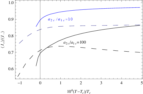
The dashed lines in Fig. 6 show the values of $bR^{2}\langle|\Delta|^{2}\rangle$ at $T=T_{c}$ and $\varphi=\varphi_{\rm max}$, evaluated by means of Eq. (14). Except for $k_{B}T_{c}\ll w/bR^{3}$ or $k_{B}T_{c}\gg w/bR^{3}$, we obtain $\langle|\Delta|^{2}\rangle\approx 0.68(bR^{2})^{-1}(k_{B}T_{c}bR^{3}/w)^{2/3}=0.68(k_{B}^{2}T_{c}^{2}/bw^{2})^{1/3}$ for $\gamma=0$. For $\gamma\rightarrow\infty$ $\langle|\Delta|^{2}\rangle$ is smaller by a factor $2^{2/3}$. The first term in the Hartree approximation value in Eq. (27) is smaller than the result obtained for $\gamma\rightarrow\infty$ by about 7%.

Figure 7 shows the average current evaluated at $T=T_{c}$ and $\varphi=\varphi_{\rm max}$. As already found in Ref. 5, $\langle I(T_{c})\rangle$ is not a monotonic function of $T_{c}$, but has a maximum instead. As discussed above, the curve for $\gamma\rightarrow\infty$ is obtained as a shift of the curve for $\gamma=0$. What we learn from this curve is that for $k_{B}T_{c}<0.163w/bR^{3}$ $|\langle I_{0}(T_{c})\rangle|>|\langle I_{\infty}(T_{c})\rangle|$, meaning that independence of the order parameters enhances the fluctuation current, whereas the opposite occurs for $k_{B}T_{c}>0.163w/bR^{3}$.

There are three material parameters that can differ between the order parameters: $a_{1c}\neq a_{2c}$, $\alpha_{1}\neq\alpha_{2}$ and $b_{1}\neq b_{2}$. Since near $T_{c}$ the usual case is $|\alpha_{1,2}\tau|,b_{1,2}|\Delta_{1,2}|^{2}\ll|a_{1c}-a_{2c}|$, we focus on the influence of the difference between $a_{1c}$ and $a_{2c}$.

Figure 8 shows the ratio between the fluctuation currents for the cases $a_{1c}\neq a_{2c}$ and $a_{1c}=a_{2c}$, while all the other parameters are kept unchanged. Although the values of $k_{B}T_{c}bR^{3}/w$ and $\gamma$ do have some influence, the general trend is that the difference between $a_{1c}$ and $a_{2c}$ inhibits fluctuation supercurrent in the region $T\approx T_{c}$, with this effect being stronger for $T<T_{c}$.