UUITP-14/11
Introduction to Graded Geometry,
Batalin-Vilkovisky Formalism and their Applications
Jian Qiua and Maxim Zabzineb
aI.N.F.N. and Dipartimento di Fisica
Via G. Sansone 1, 50019 Sesto Fiorentino - Firenze, Italy
bDepartment of Physics and Astronomy,
Uppsala university,
Box 516,
SE-751 20 Uppsala,
Sweden
These notes are based on a series of lectures given by the second author at the 31th Winter School “Geometry and Physics”, Czech Republic, Srni, January 15 - 22, 2011, and are published in Archivum Mathematicum Tomus 47 (2011), 143-199.
Abstract
These notes are intended to provide a self-contained introduction to the basic ideas of finite dimensional Batalin-Vilkovisky (BV) formalism and its applications. A brief exposition of super- and graded geometries is also given. The BV-formalism is introduced through an odd Fourier transform and the algebraic aspects of integration theory are stressed. As a main application we consider the perturbation theory for certain finite dimensional integrals within BV-formalism. As an illustration we present a proof of the isomorphism between the graph complex and the Chevalley-Eilenberg complex of formal Hamiltonian vectors fields. We briefly discuss how these ideas can be extended to the infinite dimensional setting. These notes should be accessible to both physicists and mathematicians.
1 Introduction and motivation
The principal aim of these lecture notes is to present the basic ideas about the Batalin-Vilkovisky (BV) formalism in finite dimensional setting and to elaborate on its application to the perturbative expansion of finite dimensional integrals. We try to make these notes self-contained and therefore they include also some background material about super and graded geometries, perturbative expansions and graph theory. We hope that these notes would be accessible for math and physics PhD students.
Originally the Batalin-Vilkovisky (BV) formalism (named after Igor Batalin and Grigori Vilkovisky, see the original works [4, 5]) was introduced in physics as a way of dealing with gauge theories. In particular it offers a prescription to perform path integrals of gauge theories. In quantum field theory the path integral is understood as some sort of integral over infinite dimensional functional space. Up to now there is no suitable definition of the path integral and in practice all heuristic understanding of the path integral is done by mimicking the manipulations of the finite dimensional integrals. Thus a proper understanding of the formal algebraic manipulations with finite (infinite) dimensional integrals is crucial for a better insight to the path integrals. Actually nowadays the algebraic and combinatorial techniques play a crucial role in dealing with path integral. In this context the power of BV formalism is that it is able to capture the algebraic properties of the integration and to describe the Stokes theorem as some sort of cocyle condition. The geometrical aspects of BV theory were clarified and formalized by Albert Schwarz in [24] and since then it is well-established mathematical subject.
The idea of these lectures is to present the algebraic understanding of finite dimensional (super) integrals within the framework of BV-formalism and perturbative expansion. Here our intention is to explain the ideas of BV formalism in a simplest possible terms and if possible to motivate different formal constructions. Therefore instead of presenting many formal definitions and theorems we explain some of the ideas on the concrete examples. At the same time we would like to show the power of BV formalism and thus we conclude this note with a highly non-trivial application of BV in finite dimensional setting: the proof of the Kontsevich theorem [17] about the relation between graphs and symplectic geometry.
The outline for the lecture notes is the following. In sections 2 we briefly review the basic notions from supergeometry, in particular -graded linear algebra, supermanifolds and the integration theory. As main examples we discuss the odd tangent and odd cotangent bundles. In section 3 we briefly sketch the -graded refinement of the supergeometry. We present a few examples of the graded manifolds. In sections 2 and 3 our exposition of super- and graded geometries are quite sketchy. We stress the description in terms of local coordinates and avoid many lengthy formal consideration. For the full formal exposition of the subject we recommend the recent books [26] and [6]. In section 4 we introduce the BV structure on the odd cotangent bundle through the odd Fourier transformation. We discuss the integration theory on the odd cotangent bundle and a version of the Stokes theorem. We stress the algebraic aspects of the integration within BV formalism and explain how the integral gives rise to a certain cocycle. Section 5 provides the basic introduction into the perturbative analysis of the finite dimensional integrals. We explain the perturbation theory by looking at the specific examples of the integrals in and . Also the relevant concepts from the graph theory are briefly reviewed and the Kontsevich theorem is stated. Section 6 presents the main application of BV formalism to the perturbative expansion of finite dimensional integrals. In particular we present the proof of the Kontsevich result [17] about the isomorphism between the graph complex and the Chevalley-Eilenberg complex of formal Hamiltonian vectors fields. This proof is a simple consequence of the BV formalism and as far as we are aware the present form of the proof did not appear anywhere. In section 7 we outline other application of the present formalism. We briefly discuss the application for the infinite dimensional setting in the context of quantum field theory. At the end of the notes there are a few Appendices with some technical details and proofs which we decided not to include in the main text.
2 Supergeometry
The supergeometry extends classical geometry by allowing odd coordinates, which anticommute, in contrast to usual coordinates which commute. The global objects obtained by gluing such extended coordinate systems, are supermanifolds. In this section we briefly review the basic ideas from the supergeometry with the main emphasis on the local coordinates. Due to limited time we ignore the sheaf and categorical aspects of supergeometry, which are very important for the proper treatment of the subject (see the books [26] and [6]).
2.1 Idea
Before going to the formulas and concrete definitions let us say a few general words about the ideas behind the super- and graded geometries. Consider a smooth manifold and the smooth functions over . is a commutative ring with the point-wise multiplication of the functions and this ring structure contains rich information about the original manifold . The functions which vanish on the fixed region of form an ideal of this ring and moreover the maximal ideals would correspond to the points on . In modern algebraic geometry one replaces by any commutative ring and the corresponding “manifold” is called scheme. In supergeometry (or graded geometry) we replace the commutative ring of functions with supercommutative ring. Thus supermanifold generalizes the concept of smooth manifold and algebraic schemes to include anticommuting coordinates. In this sense the super- and graded geometries are conceptually close to the modern algebraic geometry and the methods of studying supermanifolds (graded manifold) are variant of those used in the study of schemes.
2.2 -graded linear algebra
The -graded vector space over (or ) is vector space with decomposition
where is called even and is called odd. Any element of can be decomposed into even and odd components. Therefore it is enough to give the definitions for the homogeneous elements. The parity of , we denote , is defined for the homogeneous element to be if and if . If and then we will adopt the following notation and the combination is called superdimension of . Within the standard use of the terminology -graded vector space is the same as superspace. All standard constructions from linear algebra (tensor product, direct sum, duality, etc.) carry over to -linear algebra. For example, the morphism between two superspaces is -grading preserving linear map. It is useful to introduce the parity reversion functor which changes the parity of the components of superspace as follows and . For example, by we mean the purely odd vector space .
If is associative algebra such that the multiplication respects the grading, i.e. () for homogeneous elements in then we will call it superalgebra. The endomorphsim of superalgebra is a derivation of degree if
| (1) |
For any superalgebra we can construct Lie bracket as follows . By construction this Lie bracket satisfies the following properties
| (2) |
| (3) |
If in general a superspace is equipped with the bilinear bracket satisfying the properties (2) and (3) then we call it Lie superalgebra. In principle one can define also the odd version of Lie bracket. Namely we can define the bracket of parity such that (). This even (odd) Lie bracket satisfies the following properties
| (4) |
| (5) |
However the odd Lie superbracket can be mapped to even Lie superbracket by the parity reversion functor. Thus odd case can be always reduced to the even.
Coming back to the general superalgebras. The supergalgebra is called supercommutative if
The supercommutative algebras will play the central role in our considerations. Let us discuss a very important example of the suprecommutative algebra, the exterior algebra.
Example 2.1
Consider purely odd superspace over the real number of dimension . Let us pick up the basis , and define the multiplication between the basis elements satisfying . The functions on are given by the following expression
and they correspond to the elements of exterior algebra . The exterior algebra
is a supervector space with the supercommutative multiplications given by wedge product. The wedge product of the exterior algebra corresponds to the function multiplication in .
Let us consider the supercommutative algebra with the multiplication and in addition there is a Lie bracket of parity . We require that is a derivation of of degree , namely
| (6) |
Such structure is called even Poisson algebra for and Gerstenhaber algebra (odd Poisson algebra) for . It is crucial that it is not possible to reduce Gerstenhaber algebra to even Poisson algebra by the parity reversion, since now we have two operations in the game, supercommutative product and Lie bracket compatible in a specific way.
2.3 Supermanifolds
We can construct more complicated examples of the supercommutative algebras. Consider the real superspace and we define the space of functions on it as follows
If we pick up an open subset in then we can associate to the supercommutative algebras as follows
| (7) |
This supercommutative algebra can be thought of as the algebra of functions on the superdomain , . The superdomain can be characterized in terms of standard even coordinates () for and the odd coordinates (), such that . In analogy with ordinary manifolds a supermanifold can be defined by gluing together superdomains by degree preserving maps. Thus the domain with coordinates can be glued to the domain with coordinates by invertible and degree-preserving maps and defined for . Thus formally the theory of supermanifolds mimics the standard smooth manifolds. However one should anticipate that some of the geometric intuition fails and we cannot think in terms of points due to the presence of the odd coordinates. This situation is very similar to the algebraic geometry when there can be nilpotent elements in the commutative ring.
The supermanifold is defined by gluing superdomains. However, the gluing should be done with some care and for the rigorous treatment we need to use the sheaf theory. Let us give a precise definition of the smooth supermanifold.
Definition 2.2
A smooth supermanifold of dimension is a smooth manifold with a sheaf of supercommutative superalgebras, typically denoted or , that is locally isomorphic to , where is open subset of .
Thus essentially the supermanifold is defined through the gluing supercommutative algebras which locally look like in (7). This supercommutative algebra is sometimes called ’freely generated’ since it can be generated by even and odd coordinates and . If we allow more general supercommutative algebras to be glued, we will be led to the notion of superscheme which is a natural super generalization in the algebraic geometry.
Let us illustrate this formal definition of supermanifold with couple of concrete examples.
Example 2.3
Assume that is smooth manifold then we can associate to it the supermanifold odd tangent bundle, which is defined by the gluing rule
where ’s are local coordinates on and ’s are glued as . The functions on have the following expansion
and thus they are naturally identified with the differential forms, . Indeed locally the differential forms correspond to freely generated supercommutative algebra
Example 2.4
Again let be a smooth manifold and we associate to it now another super manifold odd cotangent bundle, which has the following local description
where ’s are local coordinates on and ’s transform as . The functions on have the expansion
and thus they are naturally identified with multivector fields, . Indeed the sheaf of multivector fields is a sheaf of supercommutative algebras which is locally freely generated.
Many notions and results from the standard differential geometry can be extended to supermanifolds in straightforward fashion. For example, the vector fields on supermanifold are defined as derivations of the supercommutative algebra . The use of local coordinates is extremely powerful and sufficient for most purposes. The notion of morphisms of supermanifolds can be described locally exactly as it is done in the case of smooth manifolds.
2.4 Integration theory
Now we have to discuss the integration theory for the supermanifolds. We need to define the measure and it can be done first locally in analogy with the standard case. The main novelty comes from the odd part of the measure.
Let us start from the discussion of the integration of the function in one variable. The even integral is defined as usual
| (8) |
and if we change the coordinate then the measure is changed accordingly to the standard rules . Next consider the function of one odd variable which is given by , where and are some real numbers. We define the integral over this function as linear operation such that
| (9) |
Now if we change the odd coordinate we still want the same definition to hold, namely
| (10) |
As a result of this we get that the odd measure transforms as follows and this transformation property should be contrasted with the even integration. Next we can define the odd measure over functions of many ’s. Assume that there are odd (). Using the definition for a single we define the measure to be such that
| (11) |
and all other integrals are zero. Let us change variables according to the following rule such that
In new variables we still require that
| (12) |
Therefore we obtain the following formula for the transformation of the measure, . Using these simple ideas we can define the integration of the function over any superdomain and then we have to check how the measure is glued as we patch different superdomains. On a supermanifold we would like to integrate the functions and for this we will need well-defined measure of the integration on the whole supermanifold.
Instead of writing down the general formulas let us discuss the integration of functions on odd tangent and odd cotangent bundles.
Example 2.5
Using the notation from the example 2.3 let us study the integration measure on the odd tangent bundle . The even part of the measure transforms in the standard way
while the odd part transforms according to the following property
As we can see the transformation of even and odd parts cancel each other and thus we have
which corresponds to the canonical integration on . Any function of top degree on can be integrated canonically. This is not surprising since the integration of the top differential forms is defined canonically for any smooth orientable manifold.
Example 2.6
Using the notation from the example 2.4 let us study the integration on odd cotangent bundle . The even part transforms as before
while the odd part transforms in the same way as even
Assume that is orientiable and let us pick up a volume form (nowhere vanishing top form)
One can check that transforms as a densitity
Combining all these ingredients together we can define the following invariant measure
which we can glue consistently. Thus to integrate the multivector fields we need to pick a volume form on .
3 Graded geometry
Graded geometry is -refinement of supergeometry. Many definitions from the supergeometry have straightforward generalization to the graded case. In our review of graded geometry we will be very brief, for more details one can consult [21, 11].
3.1 -graded linear algebra
A -graded vector space is a vector space with the decomposition labelled by integers
If then we say that is homogeneous element of a degree . Any element of can be decomposed in terms of homogeneous elements of a given degree. Many concepts of linear algebra and superalgebra has a straightforward generalization to the general graded case. The morphism between graded vector spaces is defined as a linear map which preserves the grading. Assuming that (or ) is vector space of degree the dual vector space is defined as . The graded vector space shifted by degree is defined as direct sum of .
If the graded vector space is equipped with the associative product which respects the grading then we call a graded algebra. The endomorphism of graded algebra is a derivation of degree if it satisfies the relation (1), but now with -grading. If for a graded algebra and any homogeneous elements and therein we have the relation
then we call a graded commutative algebra. The graded commutative algebras play the crucial role in the graded geometry. One of the most important examples of graded algebra is given by the graded symmetric space .
Definition 3.1
Let be a graded vector space over or . We define the graded symmetric algebra as the linear space spanned by polynomial functions on
where we use the relations
with and being homogeneous elements of degree and respectively. The functions on are naturally graded and multiplication of functions is graded commutative. Therefore the graded symmetric algebra is a graded commutative algebra.
In analogy with -case we can define the Lie bracket of the integer degree now such that and it satisfies the properties (4) and (5). Analogously we can introduce the graded versions of Poisson algebra. If the -graded vector space is equipped with a graded commutative algebra structure and a Lie algebra bracket of degree such that they are compatible with respect to the relation (6) then we call -graded Poisson algebra (or simply -Poisson algebra). The standard use of terminology is the following, -graded Poisson algebra is called Poisson algebra and -graded Poisson algebra is called quite often Gerstenhaber algebra. For more explanation and examples of graded Poisson algebras the reader may consult [8].
Let us make one important side remark about the sign conventions in the graded case. Quite often one has to deal with bi-graded vector spaces which carry simultaneously - and -gradings. There exist two different sign conventions when one moves one element past another,
| (13) |
and
| (14) |
where the degrees are defined as follows
Both conventions are widely used and they each have their advantages. They are equivalent, but one should never mix them while dealing the -graded superspaces. For more details see the explanation in [11]. However this sign subtlety is irrelevant for most of our consideration.
3.2 Graded manifold
We can define the graded manifolds very much in analogy with the supermanifolds. We have sets of the coordinates with assignment of degree and we glue them by the degree preserving maps. Let us give the formal definition first.
Definition 3.2
A smooth graded manifold is a smooth manifold with a sheaf of graded commutative algebras, typically denoted by , which is locally isomorphic to , where is open subset of and is graded vector space.
This definition is a generalization of supermanifold to the graded case. To every patch we associate a commutative graded algebra which is freely generated by the graded coordinates. The gluing is done by the degree preserving maps. The best way of explaining this definition is by considering the explicit examples.
Example 3.3
Let us introduce the graded version of the odd tangent bundle from the example 2.3. We denote the graded tangent bundle as and we have the same coordinates and as in the example 2.3, with the same transformation rules. The coordinate is of degree and is of degree and the gluing rules respect the degree. The space of functions is a graded commutative algebra with the same -grading as the differential forms.
Example 3.4
Analogously we can introduce the graded version of the odd cotangent bundle from the example 2.4. Now we allocate the degree for and degree for . The gluing preserves the degrees. The functions is graded commutative algebra with degree given by minus of degree of multivector field.
Example 3.5
Let us discuss a slightly more complicated example of graded cotangent bundle over cotangent bundle . In local coordinates we can describe it as follows. Introduce the coordinates , , and of degree , , and respectively. The gluing between patches is done by the following degree preserving maps
Now it is bit more complicated to describe the functions in terms of standard geometrical objects. However by construction is a graded commutative algebra. In degree zero corresponds to and in degree one to . For more details of this example the reader may consult [21].
Again the big chunk of differential geometry has a straightforward generalization to the graded manifolds. The integration theory for the graded manifolds is totally analogous to the super case, with the main difference between the even and odd measure described in subsection 2.4. The vector fields are defined as derivations of for the graded manifold . The vector fields on are naturally graded, and amongst these we are interested in the odd vector fields which square to zero.
Definition 3.6
If the graded manifold is equipped with a derivation of of degree with additional property then we call such a homological vector field. endows the graded commutative algebra of function with the structure of differential complex. One calls such graded commutative algebra with a graded differential algebra.
Let us state the most important example of homological vector field for the graded tangent bundle.
Example 3.7
Consider the graded tangent bundle described in the example 3.3. Let us introduce the vector field of degree written in local coordinates as follows
which is glued in an obvious way. Since this is an example of homological vector field. on corresponds to the de Rham differential on .
4 Odd Fourier transform and BV-formalism
In this section we introduce the basics of BV formalism. We derive the construction through the odd Fourier transformation which maps to . Odd cotangent bundle has a nice algebraic structure on the space of functions and using the odd Fourier transform we will derive the version of Stokes theorem for the integration on . The power of BV formalism is based on the algebraic interpretation of the integration theory for odd cotangent bundle.
4.1 Standard Fourier transform
Let us start by recalling the well-known properties of the standard Fourier transformations. Consider the suitable function on the real line and define the Fourier transformation of this function according to the following formula
| (15) |
One can also define the inverse Fourier transformation as follows
| (16) |
There are some subtleties related to the proper understanding of the integrals (15)-(16) and certain restrictions on to make sense of these expressions. However, let us put aside these complications in this note. The functions have associative point-wise multiplication and one can study how it is mapped under the Fourier transformation. It is an easy exercise to show that
| (17) |
where -product is defined as follows
| (18) |
This -operation is called convolution of two functions and it can be defined for any two integrable functions on the line. This -product is associative and commutative . Thus the space of integrable functions is associative commutative algebra with respect to convolution, but there is no identity (since is not an integrable function on the line). It is important to stress that the derivative is not a derivation of this -product.
4.2 Odd Fourier transform
Let us assume that the manifold is orientable and we can pick up a volume form
| (19) |
which is a top degree nowhere vanishing form and . Consider the graded manifold and the integration theory which we have discussed in the example 2.5. If we have the volume form then we can define the integration only along the odd direction as follows
In analogy with the standard Fourier transform (15) we can define the odd Fourier transfrom for as
| (20) |
where . Obviously we would like to make sense globally of the transformation (20). Therefore we assume that the degree of is and it transforms as (so in the way dual to ). Thus and the odd Fourier transform maps functions on to the functions on . The explicit formula (115) of the Fourier transform of -form is given in the Appendix. We can also define the inverse Fourier transform which maps the functions on to the functions on as follows
| (21) |
where . One may easily check that
Since we have to discuss both odd tangent and odd cotangent bundles simultaneously, in this section we adopt the following notation for the functions: we denote with symbols without tilde functions on and with tilde functions on .
is a differential graded algebra with the graded commutative multiplication and the differential defined in example 3.7. Let us discuss how these operations behave under the odd Fourier transform . Under the differential transforms to bilinear operation on as follows
| (22) |
and from this we can calculate the explicit form of
| (23) |
By construction and degree of is . Next let us discuss how the graded commutative product on transforms under . The situation is very much analogous to the standard Fourier transform where the multiplication of functions goes to their convolution. To be specific we have
| (24) |
and from this we derive the explicit formula for the odd convolution
| (25) |
where and , are odd coordinates on . This star product is associative and by construction is a derivation of this product (since is a derivation of usual product on ). Moreover we have the following relation
| (26) |
and thus this star product does not preserve -grading, i.e. . Thus the odd convolution of functions is not a graded commutative product, which should not be surprising since is not a morphism of the graded manifolds (generically it is not a morphisms of supermanifolds either). At the same time is a graded commutative algebra with respect to the ordinary multiplication of functions, but is not a derivation of this multiplication
| (27) |
We can define the bilinear operation which measures the failure of to be a derivation
| (28) |
A direct calculation gives the following expression
| (29) |
which is very reminiscent of the standard Poisson bracket for the cotangent bundle, but now with the odd momenta. For the derivative we use the following convention
and it is derivation of degree (see the definition (1)). By a direct calculation one can check that this bracket (29) gives rise to -Poisson algebra (Gerstenhaber algebra) on . Indeed the bracket (29) on corresponds to the Schouten bracket on the multivector fields (see Appendix for the explicit formulas). To summarize, upon the choice of volume form on , is an odd Poisson algebra (Gerstenhaber algebra) with the Poisson bracket generated by -operator as in (28). Such a structure is called BV-algebra. We will now summarize and formalize this notion.
Let us recall the definition of odd Poisson algebra (Gerstenhaber algebra).
Definition 4.1
The graded commutative algebra with the odd bracket satisfying the following axioms
is called a Gerstenhaber algebra.
Typically it is assumed that the degree of bracket is 1 (or depending on conventions). Thus the space of functions is a Gerstenhaber algebra with a graded commutative multiplication of functions and a bracket of degree defined by (29). The BV-algebra is Gerstenhaber algebra with an additional structure.
Definition 4.2
A Gerstenhaber algebra together with an odd –linear map
which squares to zero and generates the bracket according to
| (30) |
is called a BV-algebra. is called the odd Laplace operator (odd Laplacian).
Again it is assumed that degree is 1 (or depending on conventions). The space of functions is a BV algebra with defined by (23) and its definition requires the choice of a volume form on . The graded manifold is called a BV manifold. In general a BV manifolds is defined as a graded manifold such that the space of functions is equipped with the structure of a BV algebra.
There also exists an alternative definition of BV algebra [12].
Definition 4.3
A graded commutative algebra with an odd –linear map
which squares to zero and satisfies
| (31) | |||||
is called a BV algebra
One can show that with these properties gives rise to the bracket (30) which satisfies all axioms of the definition 4.1. The condition (31) is related to the fact that should be a second order operator, square of the derivation in other words. Consider the functions , and of one variable and the second derivative satisfies the following property
which can be regarded as a definition of second derivative. Although one should keep in mind that any linear combination satisfies the above identity. Thus the property (31) is just the graded generalization of the second order differential operator. In the example of , the as in (23) is indeed of second order.
4.3 Integration theory
So far we have discussed different algebraic aspects of graded manifolds and which can be related by the odd Fourier transformation upon the choice of a volume form on . As we saw is quite interesting algebraically since is equipped with the structure of a BV algebra. At the same time has a very natural integration theory which we will review below. Now our goal is to mix the algebraic aspects of with the integration theory on . We will do it again by means of the odd Fourier transform.
We start by reformulating the Stokes theorem in the language of the graded (super) manifolds. Before doing this let us review a few facts about standard submanifolds. A submanifold of can be described in algebraic language as follows. Consider the ideal of functions vanishing on . The functions on submanifold can be described as quotient . Locally we can choose coordinates adapted to such that the submanifold is defined by the conditions ( and ) while the rest may serve as coordinates for . In this local description is generated by . Indeed the submanifolds can be defined purely algebraically as ideals of with certain regularity condition which states that locally the ideals generated by . This construction has a straightforward generalization for the graded and super settings. Let us illustrate this with a particular example which is relevant for our later discussion. is a graded submanifold of if is submanifold of . In local coordinates is described by the conditions
| (32) |
thus generate the corresponding ideal . The functions on the submanifold are given by the quotient . Moreover the above conditions define the morphism of the graded manifolds and thus we can talk about the pull back of functions from to as going to the quotient. Also we want to discuss another class of submanifolds, namely odd conormal bundle as graded submanifold of . In local coordinate is described by the conditions
| (33) |
thus generate the ideal . Again the functions can be described as quotient . Moreover the above conditions define the morphism of the graded manifolds and thus we can talk about the pull back of functions from to .
In previous subsections we have defined the odd Fourier transformation as map
which does not map the graded commutative product on one side to the graded commutative product on the other side. Using the odd Fourier transform we can relate the following integrals over different supermanifolds
| (34) |
Let us spend some time explaining this formula. On the left hand side we integrate the pull back of over with the canonical measure , where . On the right hand side of (34) we integrate the pull back of over . The supermanifold has measure , where and we have to make sure that this measure is invariant under the change of coordinates which preserve . Indeed this is easy to check. Let us take the adapted coordinates such that () are the coordinates along and () are coordinates transverse to . A generic change of coordinates has the form
| (35) |
if furthermore we want to consider the transformations preserving then the following conditions should be satisfied
| (36) |
These conditions follow from the general transformation of differentials
| (37) |
and the Frobenius theorem which states that should only go to once restricted on . In this case the adapted coordinates transform to adapted coordinates. On we have the following transformations of odd conormal coordinate
| (38) |
Let us stress that is a coordinate on not a section, and the invariant object will be . Under the above transformations restricted to we have the following property
| (39) |
where, for the transformation of see the example 2.6. The formula (34) is very easy to prove in the local coordinates. The pull back of the functions on the left and right hand sides would correspond to imposing the conditions (32) and (33) respectively. The rest is just simple manipulations with the odd integrations and with the explicit form of the odd Fourier transform. Since all operations in (34) are covariant, i.e. respects the appropriate gluing then the formula obviously is globally defined and is independent from the choice of the adapted coordinates.
Let us recall two important corollaries of the Stokes theorem for the differential forms. First corollary is that the integral of exact form over closed submanifold is zero and the second corollary is that the integral over closed form depends only on homology class of ,
| (40) |
where and are differential forms, and are closed submanifolds which are in the same homology class. These two statements can be easily rewritten in the graded language as follows
| (41) |
| (42) |
where we assume that we deal with the pull backs of to the submanifolds.
Next we can combine the formula (34) with the Stokes theorem (41) and (42). We will end up with the following properties to which we will refer as Ward-identities
| (43) |
| (44) |
where and the pull back of these function to is assumed. One can think of these statements as a version of Stokes theorem for the cotangent bundle. This can be reformulated and generalized further as a general theory of integration over Lagrangian submanifold of odd symplectic supermanifold (graded manifold), for example see [24].
4.4 Algebraic view on the integration
Now we would like to combine the two facts about the graded cotangent bundle . From one side we have the BV-algebra structure on , in particular we have the odd Lie bracket on the functions. From the other side we showed in the last subsection that there exists an integration theory for with an analog of the Stokes theorem. Our goal is to combine the algebraic structure on with the integration and argue that the integral can be understood as certain cocycle.
Before discussing our main topic, let us remind the reader of some facts about the Chevalley-Eilenberg complex for the Lie algebras. Consider a Lie algebra and define the space of -chains as an element of . The space is spanned by
| (45) |
and the boundary operator can be defined as follows
| (46) |
where indicates the omission of the argument . Using the Jacobi identity one can easily prove that . The dual object -cochain is defined as multilinear map such that coboundary operator is defined as follows
| (47) |
and . This gives rise to the famous Chevalley-Eilenberg complex. If then we call a cocycle. If there exists such that then we call a coboundary. The Lie algebra cohomology consists the cocycles modulo coboundaries. In general we can also generalize it such that cochains take value in a -module. However this generalization is not relevant for the present discussion.
Now let us consider the generalization of Chevalley-Eilenberg complex for the graded Lie algebras. Notice in the preceding paragraph we have defined the cochain as a mapping from to numbers which is identified with . However can also be thought of as -the symmetric algebra of (see the definition 3.1). It is this formulation that allows for the most economical generalization to the graded case. Let a graded vector space equipped with Lie bracket of degree . The cochains are defined as maps from graded symmetric algebra to real numbers. More precisely, -cochain is defined as multilinear map with the following symmetry properties
| (48) |
The coboundary operator is acting as follows
| (49) | |||||
The sign factor is called the Kozul sign; it is incurred by moving to the very front. While the sign ensures that this quantity conforms to the symmetry property of (48) when exchanging . As before we use the same terminology, coboundaries and cocycles. The cohomology is -cocycles modulo -coboundaries.
Now let us consider the case where the bracket is of degree 1. The corresponding cochains and coboundary operator can be defined using the parity reversion functor applied for the even Lie algebra. Let us define be graded vector space with Lie bracket of degree . Then -cochain is defined as multilinear map with the following symmetry properties
| (50) |
The coboundary operator is acting as follows
| (51) | |||||
The formulas (50) and (51) are obtained by the parity shift from the the case with the even bracket, i.e. from the formulas (48) and (49). The cocycles, coboundaries and cohomology are defined as usual.
Now using the definition of cocycle for the odd Lie bracket let us state the important theorem about the integration which is a simple consequence of Stokes theorem for the multivector fields (43) and (44).
Theorem 4.4
Consider a collection of functions such that (). Define the integral
| (52) |
where is closed submanifold of . Then is a cocycle with respect to the odd Lie algebra structure
Moreover differs from by a coboundary if is homologous to , i.e.
where is some -cochain.
This theorem is based on the observation by A. Schwarz in [25]. Let us now present the proof of this theorem. is a graded vector space with odd Lie bracket defined in (29), and the functions with correspond to a Lie subalgebra of . The integral (52) defines a -cochain for odd Lie algebra with the correct symmetry properties
which follows from the graded commutativity of . Then the property (41) implies the following
| (53) |
Using the property of given in (28) many times, we obtain the following formula
| (54) |
where we have used . Combining (53) and (54) we obtain that defined in (52) is a cocycle, i.e.
| (55) |
where we use the definition for coboundary operator given in (51).
Next we have to show that the cocycle (52) changes by a coboundary when we deform continuously. We start by looking at the infinitesimal change of . Recall that the indices are along , while are transverse to , and is locally given by and . We parameterize the infinitesimal deformation by
where ’s parametrize the deformation. Thus a function it changes as follows
Using the bracket can be rewritten as
The first term vanishes under the integral. Specializing to infinitesimal deformation of , we have
This shows that under an infinitesimal change of , changes by a coboundary. For finite deformations of , we can parameterize the deformation as a one-parameter family . Thus we have the identity
for every , integrating both sides we finally arrive at the the formula for the finite change of
This concludes the proof of Theorem 6.1.
Now let us perform the integral (52) explicitly. Assume that the functions are of fixed degree and we will use the same notation for the corresponding multivector . After pulling back the ’s and performing the odd integration the expression (52) becomes
| (56) |
where stands for the contraction of multivector with a differential form. Here all vector fields are assumed to be divergenceless. If then this integral is identically zero, otherwise it may be non-zero and it gives rise to the cocycle on equipped with the Schouten bracket.
It is easy to construct the examples of cocycles when we restrict our attention to the vector fields only.
Example 4.5
Let us illustrate the formula (56) with a concrete set of examples. Let us pick up the volume form on and the collection of vector fields which preserve this volume form, i.e. , where is a Lie derivative with respect to . Such vector fields form the closed Lie algebra and they are automatically divergenceless. If then the integral
gives rise to the cocycle of the Lie algebra of the vector field preserving a given volume form. Such situation is realized in many examples. For instance, consider Lie group with the left invariant vector fields and left invariant volume form, Hamiltonian vector fields on Poisson manifold with unimodular Poisson structure, the Hamiltonian vector fields on symplectic manifold etc. However one should keep in mind that the corresponding cocycles are relatively trivial in some sense.
The main moral of Theorem 4.4 is that the BV integral gives rise to cocycle with specific dependence from and indeed it can be taken as a defining property of those integrals. In infinite dimensional setting when the integral is not defined at all then the statement of this Theorem can be regarded as definition. We will briefly comment on it in section 7.
5 Perturbation theory
The goal of this section is to give an introduction to the perturbative expansion of finite dimensional integrals and discuss the element of graph theory which are relevant for further discussion. We will also state the Kontsevich theorem. This section should be regarded as a technical preparation for the next section.
Gaussian integrals, though quite elementary, are really at the very core of perturbation theory. We quickly go over the Gaussian integrals on , focusing on how to organize the calculation in terms of Feynman diagrams. We will be quite brief in our discussion of the perturbative expansion. For mathematically minded reader we recommend two nice short introductions to perturbation theory, [18] and [23].
5.1 Integrals in -Gaussian Integrals and Feynman Diagrams
Let us discuss how to calculate the specific integrals on . We are interested in the combinatorial and algebraic way of the calculation of the integrals. We recall that the standard one-dimensional Gaussian integral is given by the following formula
| (57) |
The corresponding generalization for is given by
| (58) |
where is a symmetric and positive matrix. Next we introduce the generating function of -variables as follows
| (59) |
where . Let us introduce the integral
| (60) |
which is straightforward to calculate. Next we would like to discuss the following integrals
| (61) |
first if we have an odd number of ’s under the integral then it is identically zero due to symmetry properties. The integral (61) can be calculated by taking the derivatives
| (62) |
Performing the derivatives explicitly we arrive at the statement which is known in physics literature as the Wick theorem,
| (63) |
where we sum over all permutations of the indices . In general we are interested in the following integrals
| (64) |
where ’s are monomials in of the fixed degree
| (65) |
and let us assume for the moment that they are all different. Using the Wick theorem (63) we can calculate
| (66) |
where we have to contract ’s with ’s in all possible ways. The ways to contract ’s with can be depicted using the graph (Feynman diagram), where is -valent vertex and corresponds to the edges. Following physics terminology we will call a vertex and a propagator. Thus in perturbation theory, the integrals (64) are effectively organized as Feynman diagrams, and physicists have developed effective mnemonic rules to keep track of the combinatorics. Amongst these rules the symmetry factors of a Feynman diagram is the most important. Due to the close relationship between Feynman diagrams and the Kontsevich theorem about the graph complex, we spend some time to go through the examples of the Feynman diagrams. The general formula for the integral (64) looks as follows
| (67) |
where is the symmetry factor for a diagram and is the contraction of ’s with ’s according to the .
It turns out the weight of a diagram is determined by the inverse of its symmetry factor . The symmetry factor consists of three parts ,
- •
the symmetry factor of edges, if there are edges running between a pair of vertices we include a factor of .
- •
the symmetry factor of vertices, defined as the cardinality of the subgroup of that preserves the graph (disregarding the orientation of edges)
- •
in case loops (edges starting and ending on the same vertex) are allowed, a factor of 2 for each such loop
Now we present the examples which clarify and explain the formula (67)
Example 5.1
The above logic is equally applicable for one-dimensional integrals. The following integral is very easy to calculate
| (68) |
Thus we have the explicit integrals
| (69) | |||
| (70) |
In the integral (69) we have included a conventional factor of because we have two identical vertices. Now let us recalculate these integrals using the Wick theorem (63) and related combinatorics. Taking as 3 and 5-point vertices respectively, the Gaussian integral is, according to Wick’s contraction rule, summing over all possible ways of connecting all legs of the two vertices together.
The first line in Figure 1 representes the Feynman diagrams to connect to
| (71) |
where is the number of ways of contractions according to the first diagram and is the number of ways of contraction according to the second diagram. Altogether there is 15 ways of contracting with , and the number may also be calculated as follows
Furthermore we have
| (72) |
which is exactly the same as the integral (69). Indeed and are the symmetry factors for the diagrams in the first line
of Figure 1. Thus we are in agreement with the general prescription given by the formula (67).

Now let us calculate the integral with and . Altogether there are 105 ways of contracting and
Thus we have
| (73) |
where corresponds to the first diagram in the second line and to the second diagram in the second line of Figure 1. Next we get
which is exactly the same as the integral (70). Indeed and are symmetry factors for the diagrams in the second line of Figure 1. Again we have agreement with the prescription of (67).
Example 5.2
Next consider the -analogs of the previous example. Let us first calculate the following integral
| (74) |
Using the Wick theorem and the counting from the previous example we get
| (75) |
where now we have non-trivial factors
and
Moreover we can rewrite it as
| (76) |
where and are the symmetry factors for the diagrams in first line of Figure 1. Analogously we can calculate
| (77) |
which after applying the Wick theorem gives us
| (78) |
where
and
This can be rewritten as
| (79) |
where and are the symmetry factors for the diagrams in the second line of Figure 1.
In these two examples we illustrated the prescription given by the formula (67). If there are identical monomials then we have to put the additional on the left hand side for this formula to work.
So far we have assumed that the matrix is positive definite and that all integrals, considered so far, do converge. However we can treat the integrals formally and drop the condition of matrix being positive definite. Thus all our manipulations with the integrals can be merely taken as a book keeping device for Wick contractions. In all following discussion we treat the integrals formally and will not ask if the integral converges at all. Of course, we have to keep in mind that many formal integrals can be understood less formally through an analytic continuation as convergent integrals. This can be an important point if we try to go beyond the perturbative expansions.
5.2 Integrals in
As a preparation for section 6.1 we give some details of the perturbative expansion of the generalization of integrals from the previous subsection. Let be the constant symplectic form on and let be an antisymmetric non-degenerate matrix and its inverse. Let us define the formal Gaussian integral over copies of , where each copy is labeled by a subscript. The integral is defined as follows
| (80) |
where we used (58) which is now understood as formal expression. From now on, we use the summation convention that any repeated Greek indices are summed while repeated Latin indices are not summed unless explicitly indicated. In general we are interested in the following integrals
| (81) |
where are polynomials which depend on the coordinate of a copy of . Obviously it is enough to consider only monomials and we assume the following normalization
| (82) |
For physics minded readers we can comment that the above integral can be thought of as discrete field theory whose source manifold is points labeled by and target is , and whose ’fields’ are .
One can work out these integrals by usual methods,
| (83) | |||||
where we apply the Wick theorem. Thus we see clearly that the answer can be represented as Feynman diagrams (graphs), for which the Taylor coefficient of serves as vertices and serves as propagators. In this expansion the edges starting and ending at the same vertex are forbidden due to symmetry properties. This is pretty straightforward to work out, but the reader may use formula (83) to understand where does the symmetry factor come from. There is no factor for this case since all vertices are distinct. In next section we will consider this perturbation theory further in the context of BV formalism and Kontsevich theorem.
5.3 Bits of graph theory
In previous subsections we encountered the graphs which depict the rules of contracting the indices of vertexes with propagators. In physics such graphs are called Feynman diagrams. In this subsection we would like to state very briefly some relevant notions of the graph theory.
By a graph we understand a finite 1-dimensional CW complex.11 1 We recall that the CW complex is a topological space whose building blocks are cells (space homeomorphic to for some ), with the stipulation that each point in the CW complex is in the interior of one unique cell and the boundary of a cell is the union of cells of lower dimension. For example, the minimal cell decomposition of a sphere consists of one 0-cell, the north pole, and one 2-cell, containing the rest of the sphere. In simpler words, graph is collection of points (vertices) and lines (edges) with lines connecting the points. The reader may see the examples of the graphs on Figure 1. We consider only closed graphs, i.e. without external legs. The graphs depicted on Figure 1 are so called free graphs. If we number the vertices by then we will call such graph labelled graph. For every labelled graph we can construct the adjacency matrix where matrix element is equal to the number of edges between vertices and . The adjacency matrix can be used to describe the symmetries of the graph. If we relabel the vertices for a given graph then the adjacent matrix transforms by the similarity transformations , where is permutation matrix defined such if goes to under the permutation and otherwise zero. The permutation is called a symmetry if the following satisfied (or in other words and commute). Such ’s give rise to the symmetry group of the graph and the order of this group gives us which we defined previously as the symmetry factor of vertices.
An important structure of graph is its orientation. The orientation is given by
- •
ordering of all the vertices,
- •
orienting of all the edges.
If one graph with vertices of a given orientation can be turned into another after a permutation of vertices ( is the symmetry group of -elements) and flipping of edges, then we say they are equal orientation if and otherwise opposite orientation. We can talk about the oriented labelled graph, which is the labelled graph with fixed order of vertices and oriented edges. We can introduce the equivalence classes of graphs under the following relation
Thus every free graph comes with two orientations and we can now multiply the graphs (equivalence classes of graphs) by numbers and sum them formally. Thus the underlying module of the graph complex is generated by all the equivalence class of graphs, and the grading of the complex is of course the number of vertices in a graph. Quite often to represent the equivalence class of graph we will use the concrete oriented labelled graph.
We remark here that there are other orientation schemes that are equivalent to the current one. For example, the orienting of all the edges can be replaced by the ordering of all the legs from all vertices. Another convenient scheme is to order the incident legs for each vertex and order all the even valent vertices. We refer the reader to section 2.3.1 of the work [10] for the full discussion of orientation.
The graph complex comes with a differential, which acts on the graph by shrinking one edge and combining the two vertices connected by the edge. The main subtlety is to define the sign of such an operation wisely so as to make the differential nilpotent.
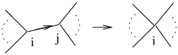
More precisely, when combining the vertices () with an edge from to , we form a new vertex named inheriting all edges landing on (except the shrunk one of course), all the vertices labeled after move up one notch, and the sign factor associated to this procedure is . Note that in [20], the vertices are labeled starting from 0 instead of 1, so the sign factor there is . In case the edge runs from to one gets an extra sign.
The graph differential makes the graphs into a chain complex , at degree the space consists of linear combinations of graphs with vertices. The graph homology is defined as the quotient of graph cycles by graph boundaries in the usual manner
And dually, we can define the graph cochain complex whose -cochains are linear mappings . We usually write this linear map as a pairing
We present the Figure 3
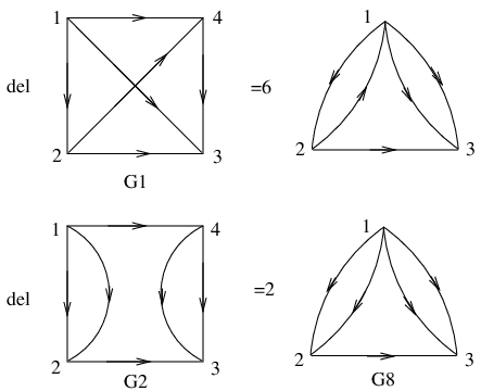
as an illustration of the graph differential. Here we use the oriented labelled graphs as representative of equivalence class. Since under the equivalence relation the edges starting and ending at the same vertex are forbidden then it is clear that we get the factor for the first line and the factor for the second line. Later on we will come back to the algebraic description of the graph differential coming from the perturbative treatment of integrals.
5.4 Kontsevich Theorem
In this subsection we review briefly the Kontsevich theorem [16, 17]. Here our presentation is quite formal and we present the theorem as certain ad hoc recipe. Later in section 6 we will rederive this theorem in much more natural fashion.
The Kontsevich theorem is about the isomorphism between the graph complex and certain Chevalley-Eilenberg complex. The Chevalley-Eilenberg complex has been reviewed in section 4.4. Here we consider the Lie algebra of formal Hamiltonian vector fields on equipped with the constant symplectic structure . The generalization to is straightforward and we leave it aside for the moment. These vector fields are generated by formal polynomial functions on
The formal Hamiltonian vector field form a closed algebra due to the relation . We are interested in the Lie algebra which contains polynomials that have only quadratic and higher terms. In particular we are interested in the Chevalley-Eilenberg complex for . Let us make the following abbreviation for the chains in this CE complex
with the boundary operator defined as usual
| (84) |
This defines the Chevalley-Eilenberg complex for which we denote . Obviously we define the dual objects, the cochains evaluating on a chain as
The Kontsevich’s theorem22 2 In fact, Kontsevich studied a relative complex which would correspond to graphs with cubic and higher vertices and it has a larger cohomology group. But as far as the mapping (85) is concerned there is no difference. states that there is an isomorphism between two complexes
| (85) |
where is graph complex defined in subsection 5.3. For any fixed , the mapping is a homomorphism, meaning it maps the graph differential into the Chevalley-Eilenberg differential. Taking the limit is for the sake of accommodating graphs with arbitrary number of vertices.
We will now give the formal recipe of the mapping (85) in detail. Given a chain from we can construct the graph chain from following steps:
- •
Fix vertices numbered from 1 to , the vertex can be maximally -valent if the polynomial has highest degree , all vertices are considered distinct but legs from one vertex are considered identical.
- •
Exhaust all possible unoriented graphs by drawing edges between vertices, one gets a collection of graphs. There are only finite number of graphs since each vertex has a maximum valency and at this stage we allow graphs containing 1- or 2-valent vertices.
- –
For each graph one assigns an arbitrary orientation to its edges, then for an edge from vertex to , one differentiates with , with and contracts with .
- –
Do this for all edges, then set all ’s to zero, the result is a c-number.
- –
Divide the c-number by (defined in subsection 5.1), this is the coefficient of the graph.
- –
- •
Doing this for all graphs one gets a linear combination of graphs.
- •
Combine coefficients of the graphs that belong to the same equivalence class (see subsection 5.3) and this give us the graph chain
We remark that step 2 can be greatly simplified, but the current low pace approach has a closer link to perturbation theory. We will give the simplified version after the next example.
The hard part is to show that the recipe gives a homomorphism, i.e. the differential in is mapped to the graph differential in under this recipe. This can be proved using methods from [10]. However there is striking similarity between the recipe given above and the Feynman diagrams in perturbative treatment of integrals. This may suggest that a simpler proof can arise from a carefully designed Gaussian integral, whose perturbative expansion naturally gives the above recipe. But there is a technical difficulty: we need to connect legs of the vertices using the inverse symplectic structure , but we cannot possibly write a Gaussian integral with since it is trivial. But let us put aside this problem for now and give instead the concrete example of the recipe where we will hopefully clarify some of the steps.
5.4.1 Example
Let be four cubic functions on with the normalization given by (82). Let us first fix to be on the vertices numbered 1,2,3,4. There are seven different ways of connecting the legs together as in Figure 4.

In fact, the last six oriented labelled graphs are related by relabeling of vertices. Following the recipe we can construct for each graph the following coefficient
In these expressions, instead of writing explicitly, we have raised indices using the inverse of symplectic structure, i.e. . And we also denote . Thus finally, the graph chain is
| (86) | |||||
The two factors 1/24 and are recognized as the total symmetry factor of (in this case loops are clearly forbidden). This is the graph chain associated with the chain .
We also see that there is a slight shortcut to the recipe above, we need only do the first two sub-steps in step 2 for one representative of an equivalence class of graphs and manually sum over anti-symmetric permutations of , then divide the result by the total symmetry factor of the graph.
Next we apply the graph differential to the chain defined in (86). We denote the bottom right graph in Figure 3 by . Then graph differential applied to (86) gives us
| (87) |
Here comes the key moment, we need to compare this result to the result obtained by applying the Chevalley-Eilenberg differential to first and the recipe above second. To do this, we write out and in (87)
| (88) | |||||
The Chevalley-Eilenberg differential acting on gives
Going back to recipe the first term gives rise to the following graph chain
and so on. Finally we get the following correspondence
which is in full agreement with (88) where we applied the graph differential explicitly.
5.5 Algebraic Description of Graph Chains
Due to the combinatorial nature of the graph complex, the proof of any proposition involving graph complex is extremely cumbersome. Therefore here we suggest a more algebraic description of the graph complex, which is motivated by the perturbative expansion of integrals. The construction involves introducing some formal parameters to represent edges and vertices in such a way that a graph corresponds to a polynomial in these parameters. These parameters have to conform to the symmetry properties of a graph, which prompts us to use odd variables ( is the number of vertices) to represent the vertices, and even variables to represent edges. We assume that in order to take the orientation of the edge into account.
Every oriented labelled graph with vertices can be represent by a monomial according to the following prescription
- •
for every vertex we include , so from all vertices we have ;
- •
for each oriented edge starting from vertex and ending at vertex , include a factor .
Let us illustrate these rules by some examples. If we look at from Figure 4 as concrete oriented labelled graph then there is the following monomial
If we multiply this monomial by then we will change the orientation of the graph. Another example is the graph from Figure 4. If is understood as oriented labelled graph then there is the following monomial
However we are interested in the equivalence classes of graphs as described in subsection 5.3. The equivalence classes can be represented by polynomials where we sum over all equivalent oriented labelled graphs (monomials). To write down a polynomial representing a graph, we follow the steps
- •
assign indices to all vertices of a graph;
- •
for each edge from vertex to , include a factor ;
- •
multiply the polynomial by and sum from 1 to .
For example, the graph in Figure 4 understood as representative of the equivalence class of graphs gives the following polynomial
While the graph in Figure 4 understood as representative of the equivalence class of graphs gives
Notice that these polynomials do not contain any symmetry factors. The point of summing over the dummy indices is so that the symmetry group acts trivially on the polynomial. Hence one such polynomial represents an equivalence class of graphs. In this formalism the orientation is taken into account automatically. Thus we can think about the graph chains as the formal polynomials in odd parameters and even parameters . Later on we will present the graph differential as formal differential operator acting on these polynomials. Many calculations drastically simplify with this algebraic description of graphs.
Sometime we will need to solve the following problem. Given polynomial in ’s and ’s we would like to know if a concrete equivalence class of graphs is present in this polynomial and if yes then which numerical factor is in front of this graph. While given a polynomial, to recover concrete equivalence class of graphs it represents we just need to do the following
- •
Pick an arbitrary graph out of an equivalence class of graphs, say, a representative whose vertices are labeled ;
- •
differentiating with respect to the odd parameters ;
- •
for each edge from vertex to , include a derivative ;
- •
set to zero all formal parameters;
- •
divide by the symmetry factor .
Observe that no summation over the dummy indices is needed. After this procedure we end up with numerical coefficient which will tell us if the equivalence class is present or not and with what factor. For example, to see if the equivalence class of from Figure 4 is present we have to apply the following operator to the polynomial
and then set all parameters to zero. For the equivalence class represented by the graph from Figure 4 the corresponding differential operator is
Note the symmetry factors for is , and for are .
We will derive later the operator corresponding to the graph differential and discuss more the algebraic description of graphs in the context of perturbative expansion.
6 BV formalism and graph complex
This section presents the non-trivial application of finite dimensional BV formalism. We will reprove the Kontsevich theorem about the relation between graph complex and Chevalley-Eilenberg complex . The existing proofs can be found in [10, 13] and in the appendix of [20] where we gave the proof generalizing Kontsevich’s theorem to the case of chord diagrams and extended Chevalley-Eilenberg complexes suited for the study of knots. The proof presented here is streamlined and simplified version of the proof from [20].
6.1 A Universal BV Theory on a Lattice
We mentioned in subsection 5.4 that the mapping from the Chevalley-Eilenberg complex to graph complex is nothing but the application of Feynman rules and that there is a technical difficulty in realizing the naive Feynman rules. We would like to construct a BV theory that circumvents this difficulty and furthermore, whose path integral gives, instead of numbers, graphs as outcome. In this way, it turns out that the Ward identity directly imply Kontsevich’s theorem. We will embed into BV formalism the perturbation theory presented in subsection 5.2.
Let us assume that the vector space is equipped with constant symplectic structure and as in subsection 5.2 we consider copies of this vector space, . We use to denote the coordinates in this big vector space, where and . Now let us construct new graded manifold
where in addition to we introduced the odd coordinates of degree . On the space of functions we can introduce the structure of BV-algebra (see the definitions 4.2 and 4.3). As in section 4.2 the odd Laplacian operator is defined as follows
The odd Poisson bracket is defined accordingly as
| (89) |
where . If we introduce then we deal with the odd cotangent bundle , where . Therefore all our previous discussion from section 4 is applicable here.
Now let us construct some specific functions on . Let us pick a function on and auxiliary odd parameters of degree (). We can construct the following function on our BV manifold
It is quite easy to see that , therefore the bracket between and is induced as
We can directly calculate the bracket
| (90) | |||||
where the bracket is the standard Poisson bracket on with respect to . Let us point out that . Next we introduce the special function which is the one we used in (81),
| (91) |
which physicists call BV action. Here are now formal degree 0 parameters with and . The purpose of introducing these parameters is to make our perturbation theory universal in the sense that the Feynman diagrams are computed as a function of .
Now we are ready to state and reprove the Kontsevich theorem discussed in subsection 5.4. Below we show that the theorem is simple consequence of BV formalims.
Theorem 6.1 (Kontsevich)
Let us take a collection of polynomial functions on and define the following integral
| (92) |
where as answer we obtain a polynomial in and which can be understood as a graph chain described in subsection 5.5. This integral can be understood as map from chain in to graph chain in . The reader can compare the perturbative expansion of the formula (92) to the recipe in section 5.4 and indeed they are the same. Moreover the map (92) satisfies the property
| (93) |
where is the Chevalley-Eilenberg differential define in (84) and is the graph differential, which has the following explicit form33 3 Here the cumbersome factor arises because we chose the number of lattice cites to be a large number and therefore we can accommodate graphs of varying number of vertices at the same time. In fact, for the current problem, one may well take and thereby eliminate this ugly factor.
| (94) |
when we deal with graph chains as polynomials (the precise definition of the operator see below in the proof).
Now we provide the proof and further explanation for this theorem. We leave to the reader to check that the perturbative expansion of (92) with the propagator
coincides with the prescription given in subsection 5.4 when we understand the answer as graph chain (i.e., formal polynomial in ’s and ’s).
We concentrate on the proof of the relation (93). For this we have to embed the integral (92) into the BV framework. Let us introduce short hand notation for the integration measure . The integral (92) can be thought as integral over odd conormal bundle
where the functions and are defined above on the BV manifold . Using the terminology from subsection 4.3 here the submanifold coincides with and thus there is no odd conormal directions left. As explained earlier in subsection 4.3, there is one single Ward identity in BV formalism (43): , we analyze its implication in the present setting
The standard manipulation with the odd Laplacian operator (28) leads to
| (95) | |||||
We observe that trivially. And furthermore all the above expressions will be restricted onto the submanifold given by and thus we can make the replacement
where we have used the relation (90). Thus we conclude that the first term of (95) gives the correlator
i.e. the correlator of the Chevalley-Eilenberg differential of . Next we analyze the last term of (95)
| (96) | |||||
Now it is best that we should explain where we are heading before we make the plunge. Focusing on the round brace, assume that is connected to in the ensuing Gaussian integral, we will get a factor
where the quantity in the first brace comes from the propagator. Summing over , we get , which renames all the into . This leads of course to
The above describes exactly the process of combining two vertices by shrinking an edge between them and letting the new vertex inherit all the other edges belonging to the two old ones. However it will be more convenient if we could write the effect of as an operator acting on the polynomial . Thus instead we proceed from (96) and perform the Gaussian integral by replacing with as in (83)
where is the short hand notation for . Letting hitting the last exponential
| (97) | |||||
We claim that this expression can be written as
| (98) |
where is a renaming operator acting on the polynomials of that renames to
To see this, again we replace with
We now commute to the left most position, picking up only a commutator
| (102) |
To proceed further, we observe that is an operator that renames the formal variables and does not touch any other index on . Its effect on the last exponential is
The last relation implies the derivation of the exponential with respect to is the same as derivation with respect to , with this we get
The summation over is now almost trivial, it can only take values because the ’s are odd. So the summation over gives times the following
This is exactly the same as (97) (upon switching ). To conclude, we have shown
Note that in the above sum, one must take the derivative first then set . This is exactly what we are after, the integral gives the graph corresponding to , and removes one edge from vertex to and renames the new vertex as inheriting all the other edges44 4 If there are originally more than one edge between and then we get zero since . While on the graph side, contracting two vertices with more than one edge in between will give loops which also leads to zero.. The sign factor is as given in subsection 5.3. We have now arrived at a neat formula
| (103) |
Thus we have completed the proof of the theorem by Kontsevich: there is a homomorphism between the Chevalley-Eilenberg complex and the graph complex given by the path integral. The proof of the homomorphism is the hard part of the theorem, while to prove that the mapping is in fact bijective is rather trivial. Suppose the dimension of the target space is big enough, one can then always find a set of polynomials, which upon applying the Feynman rules gives any given graph, this is left as an exercise for the reader.
6.1.1 Example
One can easily recast the example from subsection 5.4.1 into the calculation of the correlator according the formula (92). Now we deal with graph chains as formal polynomials.
It is instructive to show how the graph differential acts on the polynomials. Let us see the example of applying the differential operator (94) to some specific polynomials
that correspond to on Figure 4 (here these graphs are understood as equivalence classes of the graphs). A direct calculation gives (we use to denote )
To extract the coefficient of from these polynomials, one applies the operator
which can be understood as graph cochain (see Appendix C). For example
We end up with the same results as before. This is just a simple illustration how to work with the graphs as formal polynomials. We do want to point out that for concrete graphs it is much more efficient to work with pictures than to use the polynomial representation. However, the latter approach allows us to prove theorems about graph complex by manipulating operators acting on the polynomials; thus instead of drawing lots of pictures one ’lets algebra do the talking’.
6.2 Generalizations
Let us briefly sketch the possible generalizations of the above construction about the relation between certain Chevalley-Eilenberg complex and certain graph complex. As the reader may imagine there are many ways to generalize and extend the presented construction. Here we just indicate some directions and leave to the reader to figure out the details.
The most straightforward generalization is related to case of equipped with even symplectic structure
where is non-degenerate antisymmetric matrix and is symmetric matrix. Here () stands for even coordinate of and () for the odd coordinate of . In analogy with our previous discussion we can define the Chevalley-Eilenberg complex for the formal Hamiltonian vector fields on . In analogy with Theorem 6.1 we can formulate the following theorem on the relation between the Chevalley-Eilenberg complex and the graph complex .
Theorem 6.2 (super-Kontsevich)
Let us take a collection of polynomial functions , …, on and define the following integral
| (104) |
where and and
| (105) |
The integral (104) can be understood as map from chain in to graph chain in . Moreover the map (92) satisfies the property
| (106) |
where is the appropriate Chevalley-Eilenberg differential and is the graph differential defined in (94).
To understand (104) as concrete prescription we have to develop and study the perturbative expansion in the odd-coordinates. The proof of this theorem is straightforward generalization of the proof for Theorem 6.1. We have to embed the integral (104) on to BV theory on and use the Ward identities. Here the only complication compared with the previous discussion is related to some additional signs due to presence of odd coordinates ’s. We leave all these details to the reader to figure out.
By looking at Theorems 6.1 and 6.2 it is very easy to construct the graph cycles by choosing simple Chevalley-Eilenberg cycles. Let us give three different examples.
Example 6.3
Consider the case and let us choose the cubic function
such that . This is equivalent to the statement that are structure constants for some Lie algebra and is -invariant metric on this Lie algebra (here ). Using the prescription (104) we can construct the graph cycle since is trivially Chevalley-Eilenberg cycle due to property . The corresponding cycle is constructed as
| (107) |
where ’s are collection of trivalent graphs and is the number constructed by contraction of as vertices and as propagator according to the graph . The numbers satisfies so-called IHX-relations (see [3],[22]) which is equivalent to the statement that above expression is a graph cycle.
Example 6.4
Consider the standard symplectic vector space and let us choose the collection of function () such that . For example, the case would correspond to the completely integrable system on . Plug these collection of functions into the prescription of Theorem (6.1) and we will get the graph cycle since is trivially Chevalley-Eilenberg cycle due to property . The corresponding cycle has the form
| (108) |
where are numbers constructed from the contraction of vertices (Taylor coefficients of ’s) using the inverse of symplectic structure according to the graph . The concrete prescription with all numerical coefficients can be read off the perturbative expansion of (92).
Example 6.5
Now let us consider the general case and combine these two examples above. First of all we can find an odd function such that . Indeed such is related to -algebra with invariant metric (here the symplectic structure on is such a metric). The corresponding graph cycle is constructed by contracting the Taylor coefficients of as vertices and the inverse of symplectic structure as propagators. The precise prescription can be read off from the perturbative expansion of (104) which would allow as to construct graph cycle starting from a cyclic -algebra.
We can continue to play this game and construct more exotic BV theories and get more exotic graph complexes. For example, for the graph complex related to chord diagrams and the related Chevalley-Eilenberg complex see [20].
7 Outline for quantum field theory
So far our discussion involved the finite dimensional integrals and the related algebraic structures. In quantum field theory we have to study the infinite dimensional integrals and construct the corresponding BV formalism with the Ward identities. Referring to the terminology of section 4 now the manifold is infinite dimensional functional space of fields, the derivatives should be replaced by functional derivatives and formally the odd cotangent bundle should be BV manifold. However we suffer from the standard problems with infinite dimensional setting, namely some of the formulas are not well-defined and may require the additional regularization. For example, there is no simple canonical way to define the odd Lapalacian (23) in functional space since the double functional derivative is not well-defined as it stands. At the same time the odd Poisson bracket (29) can be defined in suitable way in infinite dimensional setting. Nevertheless one tries to proceed formally and apply the Ward identities (43) and (44) formally. Despite all these problems the BV formalism provides good heuristic understanding of infinite dimensional path integral. The impressive example of using BV formalism in infinite dimensional setting is given by the heuristic derivation of deformation quantization and the proof of formality in the context of Poisson sigma model, [7].
However we will not discuss the infinite dimensional BV formalism here. We restrict ourselves to a few general remark regarding the perturbative aspects of QFT. In particular we would like to concentrate on the Chern-Simons type of theories and their different relatives. We will introduce the theory in purely combinatorial fashion without any reference to infinite dimensional formulation. Since any perturbative expansion of QFT is done through the graphs (Feynman diagrams), then we would like to define certain nice objects on graphs such as element of graph homology and element of graph cohomology. The infinite dimensional path integral (partition function) will be defined as pairing of these two elements. We believe that this picture is rather generic for the perturbative expansions of QFT. However the details has been worked out only for some particular examples. Let us illustrate briefly the idea on the example of Chern-Simons theory and its different modification.
7.1 Formal Chern-Simons theory and graph cocycles
In previous section we have described how one can construct the graph cycles, see examples 6.3, 6.4 and 6.5. At the same time the QFT theory gives us a very natural and elegant way to construct the cocycles. Let us illustrate this by the example inspired by the Chern-Simons theory on (or any rational homology sphere where ). Let us consider the supermanifold with coordinates and define homological vector field . We can introduce the propagator which is smooth function defined on minus the diagonal (). The propagator satisfies the following equation
| (109) |
where is delta-function on with canonical integration. In certain sense the propagator is inverse of de Rham operator and obviously it is not uniquely defined. can be inverted on co-exact forms and thus would require the Hodge decomposition with a concrete metric. The ambiguity in (109) is given by the following formula
| (110) |
where is some function on . Assume that we choose some satisfying the above properties, then we can construct the following differential operator acting on the graph chain
| (111) |
where is understood as polynomials in and (see subsection 5.5). Thus gives a number for a given graph chain . In we replace every edge with an actual propagator running from to and every vertex with the integration over . The reader may check that in both symmetry factors of a graph are taken care of automatically. Thus the prescription (111) can be understood as way of producing the graph cochain and can be symbolically written as
| (112) |
One can prove the following statements about this cochain
- •
is well-defined;
- •
and is graph cocycle;
- •
under change (110) of the propogator , changes by coboundary ;
Thus as an element of graph cohomology is well-defined and is independent of the choice of the correlator. The proof of the first statement about being well-defined can be found in [2]. Two other statements are known, however we cannot find a complete proof of them in the literature. Thus we provide a proof of these two statement in Appendix C for any differential graded Frobenius algebra with trivial cohomology (maybe except the top degrees). The space is an example of such infinite dimensional algebra. As long as all expressions are well-defined the proofs for finite and infinite dimensional cases are identical.
Next we can take the statement of Theorems 6.1 and 6.2 about isomorphism of the Chevalley-Eilenberg complex and graph complex and by applying the differential operator (111) to (92) (or (104)) we construct the Chevalley-Eilenberg cochain
| (113) |
As a simple consequence of these theorems and the fact that is cocycle, we conclude that is the Chevalley-Eilenberg cocycle. Moreover under the change of the propagator (110) this cocycle will change by a coboundary. Thus as an element of the Chevalley-Eilenberg cohomology depends only on the concrete Frobenius algebra (here related to ). This is an example of the understanding of the infinite dimensional integral as a coycle with certain specific properties. Indeed the expression (113) can be represented as an infinite dimensional integral and the properties stated in Theorem 6.1 can be derived by some formal manipulations with this integral.
Moreover we can define the partition function as follows. Once there is a graph cocycle we can construct the Chern-Simons partition function for the Lie algebra by pairing the cocycle (111) with graph cycle constructed in the example 6.3
| (114) |
Since is graph cycle, any changes of by a coboundary vanish upon the pairing. Thus the expression is independent of the concrete choice of the propagator and it depends only on Lie algebra and the Frobenius algebra ( in the case of standard Chern-Simons theory). Thus in this sense can be though as an invariant of for fixed .
Analogously we can pair the cocycle (111) with any other graph cycles, see example 6.4 and 6.5. These will give rise to some different partition functions. For instance, the example 6.5 produces the partition function depending on cyclic -algebra and Frobenius algebra (for example, as done in [19]). This sort of models were discussed in [19] and they are natural generalizations of Chern-Simons theory.
Moreover instead of one may use any acyclic Frobenius algebra for the construction of cocycles and thus deal with the formal and discrete versions of Chern-Simons theory. For the examples of discrete version of Chern-Simons the reader may consult [9].
Depending of concrete QFT and the set of observables we may be forced to study more complicated graph complexes which can be colored, decorated, have external legs or other additional structures. However we would expect that the qualitative picture of perturbation theory as a pairing of appropriate graph cycle with graph cocycle will still hold good. These issues would require the additional study.
Acknowledgement:
M.Z. is grateful to the organizers of the Winter School for the invitation and for the warm hospitality during his stay in Czech Republic. We thank Rikard von Unge for the reading and commenting on these lecture notes. The research of M.Z. is supported by VR-grant 621-2008-4273.
Appendix A Explicit formulas for odd Fourier transform
This appendix should be regarded as companion for subsection 4.2 and we follow the same notations as in subsection 4.2. We give here some explicit formulas and derive some curious relations.
The odd Fourier transform (20) maps the differential forms to multivectors according the following explicit formula
| (115) |
where is defined as components of a nowhere vanishing top multivector field dual to the volume form (19)
The operator corresponds to the divergence operator acting on the multivector fields as follows
where we use the convention for the identification of the multivector with function on the odd cotangent bundle from the example 2.4. The odd Poisson bracket (29) corresponds to the Schouten bracket
which is the generalization of the usual Lie bracket to the multivector fields.
Let us mention a few curious facts about the transportation of the BV algebra structure to using the inverse Fourier transform (21). The graded commutative product on get mapped to the following product on
| (116) |
where and are odd coordinates on . This star product is associative product of degree and thus . The commutativity rule is and thus in general it is not a graded commutative product. If we work with -grading and is even, the product (116) is supercommutative. The odd Poisson bracket (29) gives rise to the bracket on
| (117) |
where to derive the last relation we used (22), (28) and (116). The bracket is of degree . One can easily derive the properties of the bracket on by the Fourier transform of the properties of the Gerstenhaber algebra (see the definition 4.1). Let us just point out that in the case of -grading and being even the bracket is Gerstenhaber bracket with respect to the supercommutative multiplication .
Appendix B BV-algebra on differential forms
If the manifold is equipped with a Riemannian metric then we can define the odd Fourier transform which maps to . Using the metric we can define the odd Fourier transform for as follows
| (118) |
where and is odd coordinate of degree on . If we work in superlanguage then the odd Fourier transform (118) maps to itself. In the language of differential forms the odd Fourier transform corresponds to Hodge star operation
where is -form. Under the Fourier transform the homological vector field is mapped as follows
where is defined as
| (119) |
where is the Levi-Civita connection for the metric . is operation of degree on and by construction . On the space of differential forms the operator is proportional to the adjoint of the de Rham differential, . The operator is a second order differential operator and it satisfies the relation (31) with the usual graded commutative multiplication on . Therefore the space of differential forms is equipped with the BV-structure where corresponds to and the odd bracket is
where . The integration theory is canonically defined for the differential form and thus it is not hard to extend the discussion from subsections 4.3 and 4.4 to the present case of differential forms.
The story presented here can be reiterated in many other cases, maybe with some minor modifications. For example, instead of metric we can use the symplectic structure in the definition of the odd Fourier transform (118). We can also treat in similar fashion the Lie algebroid which corresponds to a vector bundle with odd fiber coordinate and with the homological field of degree . The integration on will require some additional structure. The odd Fourier transform will map to etc. Thus we can get numerous examples of BV algebras and related structures.
Appendix C Graph Cochain Complex
The graph cochain complex is defined as a formal linear combination of dual graphs
and the evaluation of the graph cochain on a graph chain is often written as a pairing
The differential on co-graphs are defined as
Like the graph chain complex, the graph chain complex can be presented as polynomials of differential operators in
which acts on the graph polynomials in the obvious way. Instead of writing , we will just name some new formal ’dual momentum’ of , and write the polynomials of differentials as polynomials in the ’s.
In the graph chain complex case, we have a very neat homomorphism between certain Chevalley-Eilenberg complex and graph complex and this homomorphism leads us to construct graph cycles from Chevalley-Eilenberg cycles. Inspired by Chern-Simons theory Kontsevich gave a prescription of constructing graph cocycles from Frobenius algebra with some (rather strong) extra conditions. The idea is to construct out of the Frobenius algebra ’propagators’ and ’vertex functions’; then one replaces with propagators and vertex functions.
The data needed is an acyclic differential graded Frobenius algebra :
- •
is graded commutative algebra;
- •
is differential on ( and is a derivation of degree );
- •
there is non-degenerate pairing which is compatible with the graded commutative multiplication
(120) - •
the differential is compatible with pairing
(121)
Acyclic means that the cohomology of is empty, maybe except the lowest and highest degrees.
Let us give both finite and infinite dimensional examples of acyclic differential graded Frobenius algebra.
Example C.1
The finite dimensional example is given by with , where are the structure constants of the Lie algebra . The only non-zero scalar product is
note that the product is regarded as one element. This pairing is clearly graded symmetric and is non-degenerate for case. The cohomology of is trivial except .
Example C.2
Consider a rational homology -sphere (i.e., -manifold with the property for ). The space of differential forms is an infinite dimensional acyclic differential Frobenius algebra with the multiplication given by wedge and differential by the exterior derivative. The pairing is given by the integral
where and are differential forms.
Let us choose the basis for the underlying module of , let be the formal parameters corresponding to , but with no algebraic relations besides the graded commutativity.
Because of the property (120), we write the pairing suggestively as an integral
We assume that has degree , which is required to be odd (the reason will become clear later)55 5 In principle, it is enough to consider to be odd with non-homogeneous terms of different odd degrees. Although we do not know any concrete examples of this situation.. Define also the matrix
and its inverse
We denote the differential in the matrix notation as
The Stokes theorem
plus the fact that is a derivation imply
| (122) |
note we use the short hand notation where should be understood as the degree of .
With the assumption of acyclicity, may be inverted in certain sense. In fact we shall assume that the inverse of is obtained by means of Hodge decomposition. In complete analogy with the standard Hodge theory we can pick up the metric on and construct the Hodge theory for . Thus we can Hodge decompose any element into
acyclicity implies the harmonic element is zero, . The basis can be chosen as the eigen-modes of the Laplacian . The inverse can be explicitly written as
In the general case the propagator is written as
| (123) |
Here both properties of (123) follow from the symmetry properties of (122). It shall be proved later that the details of how is obtained does not affect the cohomology class of co-graphs.
Now we proceed to the construction of graph cocycles. First we define a formal integration operator that acts on polynomials of
| (124) |
We can derive the following concatenation property of the integration operator. We take copies of , and let be as in (124), but for the copy. Calculate the commutator
| (125) | |||||
Now notice the relation
from this we see (125) equals
| (126) |
This is of course the discrete version of the familiar statement
and this analogy prompts us to define
and write (126) as
| (127) |
Thus will serve as the ’ function’.
We also have the Stokes theorem
which we write concisely as
| (128) |
where on the left hand side is an operator acting on the polynomials of while on the right hand side it is the differential of the Frobenius algebra.
Consider the polynomial in , which is the generating function of the graph cochains associated with the Frobenius algebra .
| (129) |
We can deduce the properties of by using the Stokes theorem. Insert in between two exponentials,
| (130) |
Now instead of invoking Stokes theorem, we calculate by commuting to the rightmost position, doing so leaves us with only a commutator term
Naively we would conclude that the two terms in the braces cancel using the symmetry (122) and (123). But one must remember in , the index must be exact while index is co-exact (or transverse to the exact part in general). Thus the first term in the curly brace is but the index is exact while is co-exact; whereas the second term is , with co-exact and exact. To combine the two terms requires to be odd since and we get
where the sum over indices are now over both exact and co-exact ones. Now we commute this term to the left most of (130), again only picking up a commutator (using (127))
This term describes the splitting of a vertex into and . In fact, we may write as
where we have defined a splitting operator acting on the polynomial of . And we have now found the differential operator for the graph cochains
| (134) |
It is easy to see that this operator is nothing but the Fourier transform of the operator (94).
To summarize, we have shown (129) is a generating function for graph cocycles
Next we show that the cohomology class of is independent of the choice of . The propagator is the combination of the inverse of and : . The inverse of is written with the help of Hodge decomposition. Under a change of the Hodge decomposition, changes by a -exact term
In particular
Thus the corresponding change incurred in (129) is
Integrating by part, and we get
and we manipulate in similar manner
To summarize, we have shown that given an acyclic differential graded Frobenius algebra one can construct a class of graph cocycles. The explicit formula depends on the details of the propagator (Hodge decomposition), but the change of propagator only causes the graph cycle to change by coboundaries and thus the class of cocycles is completely fixed by the data of the Frobenius algebra66 6 Another proof using BV formalism was given in [14], but the authors there used the Kontsevich theorem 6.1 as an input. . However, it is not clear to us how to remove the acyclicity condition.
References
- [2] S. Axelrod and I. M. Singer, “Chern-Simons perturbation theory,” arXiv:hep-th/9110056; “Chern-Simons perturbation theory. 2,” J. Diff. Geom. 39 (1994) 173 [arXiv:hep-th/9304087].
- [3] D. Bar-Natan, “On the Vassiliev Knot Invariants.” Topology 34, 423-472, 1995.
- [4] I. A. Batalin and G. A. Vilkovisky, “Gauge Algebra And Quantization,” Phys. Lett. B 102 (1981) 27.
- [5] I. A. Batalin and G. A. Vilkovisky, “Quantization Of Gauge Theories With Linearly Dependent Generators,” Phys. Rev. D 28 (1983) 2567 [Erratum-ibid. D 30 (1984) 508].
- [6] C. Carmeli, L. Caston and R. Fioresi, “Mathematical Foundation of Supersymmetry,” with an appendix with I. Dimitrov, EMS Ser. Lect. Math., European Math. Soc., Zurich 2011.
- [7] A. S. Cattaneo and G. Felder, “A path integral approach to the Kontsevich quantization formula,” Commun. Math. Phys. 212 (2000) 591 [arXiv:math/9902090].
- [8] A. S. Cattaneo, D. Fiorenza, R. Longoni, “Graded Poisson Algebras,” Encyclopedia of Mathematical Physics, eds. J.-P. Franoise, G.L. Naber and Tsou S.T. , vol. 2, p. 560-567 (Oxford: Elsevier, 2006).
- [9] A. S. Cattaneo and P. Mnëv, “Remarks on Chern-Simons invariants,” Commun. Math. Phys. 293 (2010) 803 [arXiv:0811.2045 [math.QA]].
- [10] J. Conant and K. Vogtmann, “On a Theorem of Kontsevich,” Algebr. Geom. Topol. 3 (2003) 1167-1224, arXiv:math/0208169.
- [11] P. Deligne, J. W. Morgan, “Notes on supersymmetry (following Joseph Bernstein),” Quantum fields and strings: a course for mathematicians, Vol. 1, 2 (Princeton, NJ, 1996/1997), 41Ð97, Amer. Math. Soc., Providence, RI, 1999.
- [12] E. Getzler, “Batalin-Vilkovisky algebras and two-dimensional topological field theories,” Commun. Math. Phys. 159 (1994) 265 [arXiv:hep-th/9212043].
- [13] A. Hamilton, “A super-analogue of Kontsevich’s theorem on graph homology”, arXiv:math/0510390v1.
- [14] A. Hamilton and A. Lazarev, ”Graph cohomology classes in the Batalin-Vilkovisky formalism”, J.Geom.Phys.59:555-575,2009
- [15] G. Hochschild and J-P. Serre, ”Cohomology of Lie Algebras”, The Annals of Mathematics, Second Series, Vol. 57, No. 3 (May, 1953), pp. 591-603
- [16] M. Kontsevich, “Formal (non)-commutative symplectic geometry,Ó The Gelfand Mathematical Seminars, 1990 - 1992, Birkhäuser (1993), 173 - 187.
- [17] M. Kontsevich, “Feynman diagrams and low-dimensional topology,” First European Congress of Mathematics, 1992, Paris, Volume II, Progress in Mathematics 120, Birkhäuser 1994, 97 - 121.
- [18] M. Polyak, “Feynman diagrams for pedestrians and mathematicians,” Graphs and patterns in mathematics and theoretical physics, 15-42, Proc. Sympos. Pure Math., 73, Amer. Math. Soc., Providence, RI, 2005. [arXiv:math/0406251].
- [19] J. Qiu and M. Zabzine, “Odd Chern-Simons Theory, Lie Algebra Cohomology and Characteristic Classes,” Commun.Math.Phys. 300:789-833,2010, arXiv:0912.1243 [hep-th].
- [20] J. Qiu and M. Zabzine, ”Knot Invariants and New Weight Systems from General 3D TFTs”, J.Geom.Phys. 62:242-271, 2012, arXiv:1006.1240, hep-th.
- [21] D. Roytenberg, “On the structure of graded symplectic supermanifolds and Courant algebroids,” Quantization, Poisson brackets and beyond (Manchester, 2001), 169-185, Contemp. Math., 315, Amer. Math. Soc., Providence, RI, 2002 [arXiv:math/0203110].
- [22] J. Sawon, “Rozansky-Witten invariants of hyperkähler manifolds,” PhD thesis, Oxford 1999.
- [23] J. Sawon, “Perturbative expansion of Chern-Simons theory,” Geom. Topol. Monogr. 8 (2006) 145-166 [arXiv:math/0504495].
- [24] A. S. Schwarz, “Geometry of Batalin-Vilkovisky quantization,” Commun. Math. Phys. 155 (1993) 249 [arXiv:hep-th/9205088].
- [25] A. S. Schwarz, “Quantum observables, Lie algebra homology and TQFT,” Lett. Math. Phys. 49 (1999) 115 [arXiv:hep-th/9904168].
- [26] V. S. Varadarajan, “Supersymmetry for mathematicians: an introduction,” Courant Lecture Notes Series, AMS, New York, 2004.