Open inflation in the landscape

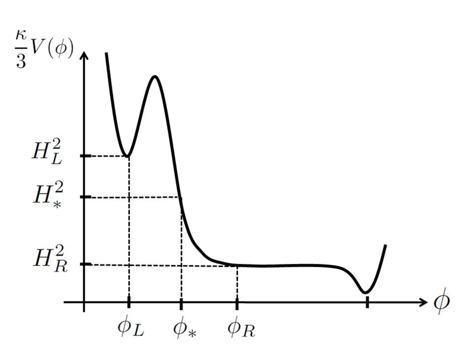
The system which we are going to consider consists of a minimally coupled scalar field, $\phi$ with Einstein gravity. As we mentioned in Sec I, the most important cosmological consequence in the string landscape was that there was a tunneling event in our past. Let us consider an effective potential $V(\phi)$ with a local minimum at $\phi_{\rm L}$, a slow-roll inflationary plateau at $\phi_{\rm R}$ and a point where the field emerges at $\phi_{*}$, as shown in Fig. 1. The action is given by

In this paper, we assume that the final tunneling transition occurs through the CDL instanton. Let us consider the $O(4)$-symmetric bounce solution [6, 7]. An $O(4)$-symmetric bubble nucleation is described by the Euclidean solution (instanton). The metric is given by

and the background scalar field is denoted by $\phi=\phi(t_{\rm E})$.

The Euclidean background equations are given by

where a dot represents differentiation with respect to $t_{\rm E}$.

The background geometry and the field configuration in the Lorentzian regime are obtained by the analytic continuation of the bounce solution. It is convenience to use the coordinate $\eta$ defined by ${\rm d}t=a(\eta){\rm d}\eta$. The coordinates in the Lorentzian regime are given by (see e.g. [34, 13])

The Penrose diagram for this open Friedmann-Robertson-Walker universe is presented in Fig. 2.

Typically, CDL instantons exist only if $V^{\prime\prime}>\kappa V$ [22]. This condition, in combination with the requirement of the subsequent long stage of the slow-roll inflation, requires a very special choice of potentials in the single-field models [26, 27]. Alternatively, one may consider multifield models [20, 35, 37, 36, 40].

In this paper, we will concentrate on the single-field models and assume that the CDL instanton exists. Meanwhile, inflation typically requires $V^{\prime\prime}\ll\kappa V$. It is difficult to make these two conditions compatible. Therefore one may expect that the slow-roll inflation does not start immediately after the CDL tunneling, and there must be some intermediate stage of rapid rolling down [26, 27].

This intermediate regime may last for a long time if the field potential is steep after tunneling. In general, this may be a typical situation during the tunneling in the string landscape scenario. As we mentioned in the introduction, the tunneling in the landscape may occur from a metastable vacuum with a very high value of energy density. Unless we have some specific knowledge about this vacuum state, one may assume that the scale of the energy density of this vacuum may be $O(1)$ in Planck units, or it may take some value on the grand unification energy scale $\sim 10^{-10}$. Meanwhile in many models of the slow-roll inflation based on string theory with vacuum stabilization, the Hubble constant must be smaller than the gravitino mass [42]. Although it is possible to avoid this conclusion, it is very hard to do it without fine-tuning. If the gravitino mass is of the order $1$ TeV or lower, the corresponding vacuum energy density during the last stage of the slow-roll inflation should be smaller than $10^{-30}$, in Planck units.

Our knowledge of the string landscape is very incomplete, so one should not fully rely on the estimates given above. However, on the basis of our present understanding of the situation, one should not be surprised to have a very long-lasting noninflationary stage after tunneling, which should last until the large energy density of the metastable vacuum state is reduced by many orders of magnitude and the slow-roll inflation begins. We will show that the behavior in the phase of the rapid rolling down significantly affects the CMB power spectrum. In the next subsection, we will investigate the field evolution inside the open universe in the region R in Fig. 2.

In order to study the field dynamics inside the light cone emanating from the center of the bubble (region R), it is useful to use the following identity:

where $\rho_{\phi}=\dot{\phi}^{2}/2+V$, $p_{\phi}=\dot{\phi}^{2}/2-V$ and $w_{\phi}\equiv p_{\phi}/\rho_{\phi}$. The asymptotic boundary conditions at the nucleation point are given by

Thus, we have

where we have introduced

and $\epsilon_{*}=\epsilon(\phi_{*})$. We have also introduced $H_{*}^{2}\equiv\kappa V(\phi_{*})/3$, which is not the expansion rate at $t=0$. This suppressed decreased rate of the energy density at around $t=0$ is caused by the large Hubble friction due to the spatial curvature term. Hence, the field at $t\approx 0$ rolls slowly even if the potential is steep. As the spatial curvature term decays, eventually the potential energy starts to dominate or the energy density starts to decay. The potential dominance starts at $t\approx H_{*}^{-1}$ while the decay of the energy density starts when $1+w_{\phi}$ becomes $O(1)$, i.e. at $t\approx\epsilon_{*}^{-1/2}H_{*}^{-1}$. Thus, the scenario changes depending on whether $\epsilon_{*}$ is large or small compared with unity. It is shown in Fig. 3 schematically how the evolution of the energy density depends on $\epsilon_{*}$, assuming that $\epsilon$ stays constant until the field falls down to a plateau of the potential.

First, we consider the case with $\epsilon_{*}\ll 1$. In this case potential energy starts to dominate at $t\approx H_{*}^{-1}$ after a short curvature dominated stage, and there is no rapid-roll regime. Once the potential term dominates, $1+w_{\phi}$ becomes ${\cal O}(\epsilon)$ as usual. Then, the energy density of the field decays slowly unless the potential becomes steep again at a later stage.

In contrast, if the potential is steep at the nucleation point, i.e. $\epsilon_{*}\geq 1$, the situation is different. As one can see from Eq. (11), $1+w_{\phi}$ becomes ${\cal O}(1)$ at $t\approx\epsilon_{*}^{-1/2}H_{*}^{-1}$ before the potential starts to dominate. The energy density of the field starts to decay rapidly proportional to $a_{\rm R}^{-3(1+w_{\phi})}$. During this rapid-roll phase, $1+w_{\phi}$ is estimated as

where we have used $\dot{\phi}={\cal O}(V^{\prime}/H)$. One can see that the rapid-roll phase lasts as far as $\epsilon\gg H^{2}/\kappa V(\gtrsim 1)$. When the field falls down to a plateau of the potential, the velocity of the field eventually decreases. Then, the slow-roll inflation starts and the curvature term becomes completely irrelevant for the background expansion of the universe. We denote the Hubble parameter at the onset of this slow-roll phase by $H_{\rm R}$.

An interesting feature of the dynamics for a steep slope is “tracking”, which means that the ratios among the kinetic term, the potential term and the curvature term are approximately constant. Suppose $\epsilon(\phi)$ is a constant for simplicity. This is exactly realized when the potential is exponential-type:

To see that an exact tracking solution exists in this case, we solve Eqs. (3), (4) and (5) under the assumption

Only if $\epsilon_{*}>1$, can one solve these equations consistently to find

It is obvious that the above solution is an exactly tracking solution. Furthermore, one can show that it is an attractor solution.

We should note that the tracking occurs even for $\epsilon_{*}={\cal O}(1)$. The difference from the case with $\epsilon_{*}\gg 1$ is that the curvature term is subdominant for the expansion of the universe in this case during the tracking phase. This means that the curvature length is well outside the horizon scale for $\epsilon_{*}={\cal O}(1)$, while it remains comparable to the horizon scale for $\epsilon_{*}\gg 1$.

The above simplest example does not have a transition to the late-time slow-roll phase. Here we introduce two simple toy models, which have the transition from the initial rapid-roll phase to the late-time slow-roll phase, and we discuss the tensor perturbation in these models later.

The first model has the effective potential of the following type:

with $H_{*}\gg H_{R}$. The potential of a similar type often appears in supergravity and superstring theory. As a concrete example, we will choose the parameters $H_{*}^{2}=10^{-3}M_{\rm pl}^{2}$, $H_{\rm R}^{2}=10^{-30}M_{\rm pl}^{2}$ and $\phi_{*}=10M_{\rm pl}$. In Fig. 4, the time evolution of the energy densities for $\epsilon_{*}=0.1$, $0.5$, $1$, $10^{2}$ and $10^{4}$ is shown. As is expected, for $\epsilon_{*}<1$ the field starts to decay slowly at $t\approx H_{*}^{-1}$, for $\epsilon_{*}\geq 1$ it starts to fall down toward the slow-roll plateau at $t=\epsilon_{*}^{-1/2}H_{*}^{-1}$ and its energy density decays in proportion to $1/a_{\rm R}^{2}$, i.e. tracking.

The second model is a variant of the potential for the chaotic inflation:

The slow-roll parameter is given by

Note that we will impose $\kappa\phi_{\rm R}^{2}>8$ for the slow-roll inflation to occur at $\phi=\phi_{\rm R}$. As with the exponential-type potential, the potential of a similar type also often appears in supergravity and superstring theory. As a concrete example, we will consider the case with $H_{\rm R}^{2}=10^{-40}M_{\rm pl}^{2}$ and $\phi_{\rm R}=7.5M_{\rm pl}$. In Fig. 5, the evolution of the energy densities for $\phi_{*}=9\phi_{\rm R}$, $7\phi_{\rm R}$, $5\phi_{\rm R}$, and $3\phi_{\rm R}$ is shown. Since the field varies slowly near the nucleation point, the chaotic-type potential Eq. (19) can be approximated there by the exponential-type. Therefore one can see that the tracking solution appears after $t\approx\epsilon_{*}^{-1/2}H_{*}^{-1}$ even in this chaotic-type potential.

We begin with reviewing how to compute the CMB power spectrum due to tensor perturbation for single-field models of one-bubble open inflation, following Refs. [32, 33]. Assuming that the observer is at the center of the spherical coordinates, the relevant tensor perturbation is the even parity one. We introduce the variable $U_{p}$ to expand the spatial metric perturbation

where $\hat{a}^{({\rm T})}_{p\ell m}$ and $Y^{(+)p\ell m}_{ij}$ denote the annihilation operator and the analytic continuation of the even parity tensor harmonics on the 3-hyperboloid [43], respectively. The function $Y^{(+)p\ell m}_{ij}$ is more explicitly expressed using the ordinary spherical harmonics $Y_{lm}$. In the Sachs-Wolfe formula we only need the $\chi\chi$ component, which is given by

Then, the time evolution equation for $f^{p\ell}(\chi_{\rm C})$ is in a model-independent manner given by

As a natural vacuum state after tunneling, we adopt the Euclidean vacuum, which is specified by requiring that the positive frequency functions are all regular at $\chi_{\rm C}=0$. Then, we have

where $P^{\mu}_{\nu}$ is the associated Legendre function of the first kind. We have fixed the normalization constant so that the analytic continuation of $Y^{p\ell m}(\chi_{\rm C},\Omega)\equiv f^{p\ell}(\chi_{\rm C})Y_{\ell m}(\Omega)$ to region R or L behaves as a spatial harmonic function properly normalized on a unit 3-hyperboloid.

The equation for $U_{p}$ is the same as the one for the massless scalar field [28]:

It is also convenient to introduce another variable ${\bm{w}}^{p}$, which is related to $U_{p}$ by [32, 33]

Then, the spatial eigenfunction ${\bm{w}}^{p}$ satisfies a simple equation

with

where a prime represents differentiation with respect to the conformal time. Since the effective potential $U_{\rm T}$ is clearly positive definite, there is no supercurvature mode (bound state) in the tensor-type perturbation.

From the boundary conditions for the background solution, we find that the potential $U_{T}$ vanishes at both boundaries of the region C. Hence, the asymptotic solutions of ${\bm{w}}^{p}$ are given by plane waves. We take the two orthogonal solutions ${\bm{w}}^{p}_{{\rm C}(\pm)}$ having the asymptotic behavior

as independent solutions. The reflection and transmission coefficients satisfy the Wronskian relations:

Using the relation between the coordinates (6), we analytically continue Eq. (27) to the region R. Then, we obtain the evolution equation for ${\bm{w}}^{p}$,

Similarly, the analytic continuations of the two independent modes to the region R are given by

where $\tilde{\bm{w}}^{p}$ is the solution of Eq. (33) that asymptotically behaves like $\tilde{\bm{w}}^{p}\rightarrow e^{ip\eta_{\rm R}}$ in the limit $\eta_{\rm R}\rightarrow-\infty$. The amplitude of the fluctuation is proportional to the sum of squares of these two independent modes, which is evaluated as

After the horizon crossing, $a^{2}H^{2}\gg p^{2}+1$, Eq. (25) implies that the amplitude of $U_{p}$ freezes. In terms of ${\bm{w}}^{p}$, two independent solutions after the horizon crossing are given by

Neglecting the decaying mode ${\bm{w}}^{p}_{1}$, we denote the asymptotic behavior of $\tilde{\bm{w}}^{p}$ as

where ${\mathbb{H}}_{p}$ and $\eta_{\rm T}^{p}$ are the amplitude and phase, respectively. We note that $p\eta_{\rm T}^{p}$ vanishes in the limit $p\rightarrow 0$ because $\overline{\tilde{\bm{w}}^{p}}=\tilde{\bm{w}}^{-p}$.

Using ${\mathbb{H}}_{p}$ and $\eta_{\rm T}^{p}$, the even parity tensor power spectrum can be expressed as [32, 33]

where

essentially represents the effects of the bubble wall.

To summarize, in order to find the power spectrum for tensor-type perturbations, one has to solve the scattering problem (27) in the region C to obtain $\rho_{+}^{p}$ and the evolution equation (38) in the region R to obtain ${\mathbb{H}}_{p}$ and $\eta_{\rm T}^{p}$.

Our main focus in this paper is on the latter process. Investigating the various possibilities for the tunneling potential is beyond the scope of this paper. We simply use the known results under thin-wall approximation [29]. For a thin-wall bubble, the effective potential $U_{\rm T}$ is characterized by two constant parameters, $\eta_{\rm W}$ and $\Delta s$:

It can be shown that $\eta_{\rm W}$ and $\Delta s$ are expressed in terms of the vacuum energies and the surface tension of the wall, $S_{1}=\int{\rm d}t_{\rm C}\dot{\phi}^{2}$, as

with

where $H_{\rm L}=\sqrt{\kappa V(\phi_{\rm L})/3}$ and $H_{*}=\sqrt{\kappa V(\phi_{*})/3}$.

In terms of $\eta_{\rm W}$ and $\Delta s$, we can solve the equation for the mode function (27) to obtain the reflection coefficient $\rho_{+}$:

From Eq. (32), the transmission probability from the false vacuum is given by $\bigl|\sigma_{+}^{p}\bigl|^{2}=1/[1+(\Delta s/2p)^{2}]$. From this expression, we find that efficiently reflected at the wall are only low frequency modes with $p\lesssim\Delta s/2$, which are thought to be interpreted as the wall fluctuation [29]. Notice that the reflection rate at $p=0$ is unity. Without this reflection by the wall, the square amplitude of fluctuation is divergent. In this sense, one might be able to interpret that the so-called wall fluctuation mode represents the penetration of the waves from the false vacuum side, and its amplitude is reduced if the wall efficiently reflects back the waves. Substituting the expression (45), the spectrum becomes

where $b_{p}:=2\left(\eta_{\rm W}-\eta_{\rm T}^{p}\right)$. Once parameters $\eta_{\rm W}\,,\Delta s$ and the late-time asymptotic value of $\tilde{\bm{w}}^{p}$ are fixed, we can immediately calculate the power spectrum using this formula. The power spectra for the tensor-type perturbation are shown in Fig. 6 for $(\alpha,\beta)=(100,1)$, $(1,100)$, $(10^{-3},10^{-3})$ and $(1,1)$, setting ${\mathbb{H}}_{p}=H_{R}$ and $\eta_{T}^{p}=0$. As a reference, we plot the spectrum for ${\mathbb{H}}_{p}=H_{R}$, $\Delta s=\infty$ and $b_{p}=0$, which we denote by “plain spectrum” in this paper, as a dashed curve in black in the same figure.

Now we move on to the problem of solving the evolution equation (38) in the region R to evaluate ${\mathbb{H}}_{p}$ and $\eta_{\rm T}^{p}$.

We translate the spectrum for tensor-type perturbation obtained in the preceding subsection into CMB temperature anisotropies, following the discussion given in Ref. [29]. The large-angle CMB temperature anisotropies due to tensor-type perturbation are simply evaluated by the Sachs-Wolfe formula

where $\eta_{0}$ and $\eta_{\rm LSS}$, respectively, denote the conformal time at the present epoch and that at the last scattering surface, $\hat{n}^{i}$ is the unit vector along the observer’s line of sight and $x^{i}(\eta)=(\eta_{0}-\eta)\ \hat{n}^{i}$ represents the photon trajectory.

Since we are interested in the anisotropies on large angular scales, we consider only those modes that enter the Hubble horizon after the universe becomes matter dominated. Thus, we set the scale factor to $a(\eta)=\cosh\eta-1$. The conformal time then can be written in terms of the density parameter $\Omega_{0}$ and the redshift $z$:

where we have neglected the effect of the dark energy.

The evolution equation for $U$ is given by [44]

The above equation can be solved exactly to give

where $U_{p}(0)$ is the initial amplitude of fluctuations given by Eq. (39) and

is the growing mode function. Now, we decompose the temperature anisotropies in terms of the spherical harmonics:

where

and the radial-radial component of the tensor-type harmonic function $Y^{p\ell m}_{\chi\chi}(\chi,\Omega)$ is given by

The temperature anisotropies are usually expressed in terms of $C_{\ell}$, the multipole moments of the temperature autocorrelation function, defined by

where $\cos\theta=\hat{\bm{n}}\cdot\hat{\bm{n}}^{\prime}$. Then, the multipole moments for the tensor-type perturbation $C^{({\rm T})}_{\ell}$ are given by

We will discuss possible observational signatures in the CMB temperature anisotropies in the open inflation scenario revived in the context of string theory landscape that prefers a moderately small value of $1-\Omega_{0}$. The value of $\Omega_{0}$ depends rather sensitively on the underlying scenario. The prediction for the value of $\Omega_{0}$, based on the primordial distribution of the number of the e folds of the inflation inside the bubble and the anthropic bias, was investigated in [17, 19]. There is a big uncertainty because the resulting distribution of the value of $\Omega_{0}$ strongly depends on the choice of the probability measure, but their estimates imply that it can be natural that $1-\Omega_{0}$ is in the marginally observable range. For this reason, we focus on the case that $1-\Omega_{0}$ is in the observable range, e.g. from $10^{-3}$ to $10^{-2}$, and evaluate the CMB anisotropies for the previously introduced two toy models.

The computed CMB temperature power spectra for the exponential-type and chaotic-type models are shown in Figs. 9 and 10, respectively. Again we set $\alpha=1$ and $\beta=1$ as a representative case in which the contribution from the wall fluctuation mode is negligibly small. One can see that the tensor CMB angular power spectrum for small $\ell$ behaves like $(1-\Omega_{0})^{\ell}$, while it agrees with the scale invariant inflationary tensor spectrum for large $\ell$. Compared with the amplitude of the tensor perturbation for the slow-roll inflation at $H\approx H_{R}$, there is significant enhancement for small $\ell$ due to the field dynamics in the region R for $\epsilon_{*}\lesssim 1$. Hence, we find that, unless $\epsilon$ is not extremely large, rapid rolling down affects the CMB spectrum at low $\ell$ significantly.

It is known that the spectrum Eq. (57) can be approximately decomposed into two pieces:

where $P_{\rm W}\,\tilde{C}_{\ell}^{({\rm W})}$ represent contributions due to wall fluctuations:

We have also introduced $C_{\ell}^{({\rm T},{\rm res})}$, which corresponds to the continuous spectrum due to standard tensor perturbations, as the residual piece of the spectrum. The previous plots presented in Figs. 9 and 10 are basically corresponding to $C_{\ell}^{({\rm T},{\rm res})}$.

The effect of the wall fluctuation mode is rather easy to investigate analytically, and in many cases it is more important than the continuum modes. To see observational signatures when the deviation of $\Omega_{0}$ from unity is small, it will be useful to expand quantities with respect to $1-\Omega_{0}$. The spectrum due to the wall fluctuations given by Eq. (60) reduces to

Unless $1-\Omega_{0}$ is close to unity, the effects of wall fluctuation mode mainly appear in the quadrupole of CMB temperature fluctuation.

The amplitude of the wall fluctuation mode can be also evaluated analytically. As seen in Figs. 6, 7, and 8, the integral (60) is dominated by the contribution from $p$ around 0. Thus, we expand $P_{\rm T}(p)$ around $p=0$ as

References

- [1] E. Komatsu et al., “Seven-Year Wilkinson Microwave Anisotropy Probe (WMAP) Observations: Cosmological Interpretation,”, Astrophys. J. Suppl. Ser. 192, 18 (2011), arXiv:1001.4538 [astro-ph.CO].
- [2] A. D. Linde, Particle Physics and Inflationary Cosmology (Harwood, Chur, Switzerland, 1990) [arXiv:hep-th/0503203].
- [3] S. Kachru, R. Kallosh, A. Linde and S. P. Trivedi, “De Sitter vacua in string theory,” Phys. Rev. D 68, 046005 (2003) [arXiv:hep-th/0301240].
- [4] L. Susskind, in Universe or Multiverse?, edited by B. Carr (Cambridge University Press, Cambridge, England, 2007), p247
- [5] B. Freivogel and L. Susskind, “A framework for the landscape,” Phys. Rev. D 70, 126007 (2004) [arXiv:hep-th/0408133].
- [6] S. R. Coleman, “The Fate Of The False Vacuum. 1. Semiclassical Theory,” Phys. Rev. D 15, 2929 (1977) [Erratum-ibid. D 16, 1248 (1977)].
- [7] S. R. Coleman and F. De Luccia, “Gravitational Effects On And Of Vacuum Decay,” Phys. Rev. D 21, 3305 (1980).
- [8] J. R. Gott, “Creation Of Open Universes From De Sitter Space,” Nature 295, 304 (1982).
- [9] J. R. Gott and T. S. Statler, “Constraints On The Formation Of Bubble Universes,” Phys. Lett. B 136, 157 (1984).
- [10] M. Sasaki, T. Tanaka, K. Yamamoto and J. Yokoyama, “Quantum state inside a vacuum bubble and creation of an open universe,” Phys. Lett. B 317, 510 (1993).
- [11] B. Ratra, P. J. E. Peebles, “Inflation in an open universe,” Phys. Rev. D52, 1837-1894 (1995).
- [12] M. Bucher, A. S. Goldhaber and N. Turok, “An open universe from inflation,” Phys. Rev. D 52, 3314 (1995) [arXiv:hep-ph/9411206].
- [13] M. Sasaki, T. Tanaka and K. Yamamoto, “Euclidean vacuum mode functions for a scalar field on open de Sitter space,” Phys. Rev. D 51, 2979 (1995) [arXiv:gr-qc/9412025].
- [14] D. H. Lyth and A. Woszczyna, Phys. Rev. D 52, 3338 (1995) [arXiv:astro-ph/9501044].
- [15] K. Yamamoto, M. Sasaki and T. Tanaka, “Large angle CMB anisotropy in an open university in the one bubble inflationary scenario,” Astrophys. J. 455, 412 (1995) [arXiv:astro-ph/9501109].
- [16] M. Bucher and N. Turok, “Open Inflation With Arbitrary False Vacuum Mass,” Phys. Rev. D 52, 5538 (1995) [arXiv:hep-ph/9503393].
- [17] B. Freivogel, M. Kleban, M. Rodriguez Martinez, L. Susskind, JHEP 0603, 039 (2006). [hep-th/0505232].
- [18] S. Weinberg, “Anthropic Bound on the Cosmological Constant,” Phys. Rev. Lett. 59, 2607 (1987).
- [19] A. De Simone and M. P. Salem, “The distribution of from the scale-factor cutoff measure,” Phys. Rev. D 81, 083527 (2010) [arXiv:0912.3783 [hep-th]].
- [20] A. D. Linde, “Inflation with variable ,” Phys. Lett. B 351, 99 (1995) [arXiv:hep-th/9503097]; A. D. Linde and A. Mezhlumian, “Inflation with ,” Phys. Rev. D 52, 6789 (1995) [arXiv:astro-ph/9506017].
- [21] S. W. Hawking and I. G. Moss, “Supercooled Phase Transitions In The Very Early Universe,” Phys. Lett. B 110, 35 (1982).
- [22] L. G. Jensen and P. J. Steinhardt, “Bubble Nucleation And The Coleman-Weinberg Model,” Nucl. Phys. B 237, 176 (1984).
- [23] A.A. Starobinsky, in: Fundamental Interactions (MGPI Press, Moscow, 1984), p. 55; A.A. Starobinsky, in: Current Topics in Field Theory, Quantum Gravity and Strings, Lecture Notes in Physics, eds. H.J. de Vega and N. Sanchez (Springer, Heidelberg 1986) 206, p. 107.
- [24] A. D. Linde, “Hard art of the universe creation (stochastic approach to tunneling and baby universe formation),” Nucl. Phys. B 372, 421 (1992) [arXiv:hep-th/9110037].
- [25] P. Batra and M. Kleban, “Transitions Between de Sitter Minima,” Phys. Rev. D 76, 103510 (2007) [arXiv:hep-th/0612083].
- [26] A. D. Linde, “A toy model for open inflation,” Phys. Rev. D 59, 023503 (1998) [arXiv:hep-ph/9807493].
- [27] A. D. Linde, M. Sasaki and T. Tanaka, “CMB in open inflation,” Phys. Rev. D 59, 123522 (1999) [arXiv:astro-ph/9901135].
- [28] T. Tanaka and M. Sasaki, “The spectrum of gravitational wave perturbations in the one-bubble open inflationary universe,” Prog. Theor. Phys. 97, 243 (1997) [arXiv:astro-ph/9701053].
- [29] M. Sasaki, T. Tanaka and Y. Yakushige, “Wall fluctuation modes and tensor CMB anisotropy in open inflation models,” Phys. Rev. D 56, 616 (1997) [arXiv:astro-ph/9702174].
- [30] M. Bucher, J. D. Cohn, “Primordial gravitational waves from open inflation,” Phys. Rev. D55, 7461-7479 (1997). [astro-ph/9701117].
- [31] T. Hertog, N. Turok, “Gravity waves from instantons,” Phys. Rev. D62, 083514 (2000). [astro-ph/9903075].
- [32] J. Garriga, X. Montes, M. Sasaki and T. Tanaka, “Spectrum of cosmological perturbations in the one-bubble open universe,” Nucl. Phys. B 551, 317 (1999) [arXiv:astro-ph/9811257].
- [33] J. Garriga, X. Montes, M. Sasaki and T. Tanaka, “Canonical quantization of cosmological perturbations in the one-bubble open universe,” Nucl. Phys. B 513, 343 (1998) [arXiv:astro-ph/9706229].
- [34] K. Yamamoto, M. Sasaki and T. Tanaka, “Quantum fluctuations and CMB anisotropies in one-bubble open inflation models,” Phys. Rev. D 54, 5031 (1996) [arXiv:astro-ph/9605103].
- [35] M. Sasaki and T. Tanaka, “Can the simplest two-field model of open inflation survive?,” Phys. Rev. D 54, R4705 (1996) [arXiv:astro-ph/9605104].
- [36] J. Garcia-Bellido, “Open inflation models and gravitational wave anisotropies in the CMB,” Phys. Rev. D 56, 3225 (1997) [arXiv:astro-ph/9702211].
- [37] A. M. Green and A. R. Liddle, “Open inflationary universes in the induced gravity theory,” Phys. Rev. D 55, 609 (1997) [arXiv:astro-ph/9607166].
- [38] J. Garriga and V. F. Mukhanov, “On classical anisotropies in models of open inflation,” Phys. Rev. D 56, 2439 (1997) [arXiv:astro-ph/9702201].
- [39] J. Garcia-Bellido, J. Garriga and X. Montes, “Quasi-open inflation,” Phys. Rev. D 57, 4669 (1998) [arXiv:hep-ph/9711214].
- [40] J. Garcia-Bellido, “Single-bubble open inflation: An overview,” arXiv:hep-ph/9803270.
- [41] J. Garcia-Bellido, J. Garriga and X. Montes, “Microwave background anisotropies in quasiopen inflation,” Phys. Rev. D 60, 083501 (1999) [arXiv:hep-ph/9812533].
- [42] R. Kallosh and A. Linde, “Landscape, the scale of SUSY breaking, and inflation,” JHEP 0412, 004 (2004) [arXiv:hep-th/0411011].
- [43] K. Tomita, Prog. Theor. Phys. 68, 310 (1982)
- [44] H. Kodama and M. Sasaki, Prog. Theor. Phys. Suppl. 78, 1 (1984)
- [45] C. R. Contaldi, M. Peloso, L. Kofman, A. D. Linde, “Suppressing the lower multipoles in the CMB anisotropies,” JCAP 0307, 002 (2003). [astro-ph/0303636].