Thermal Instability in Gravitationally-Stratified Plasmas: Implications for Multi-Phase Structure in Clusters and Galaxy Halos
Abstract
We study the interplay among cooling, heating, conduction, and magnetic fields in gravitationally-stratified plasmas using simplified, plane-parallel numerical simulations. Since the physical heating mechanism remains uncertain in massive halos such as groups or clusters, we adopt a simple, phenomenological prescription which enforces global thermal equilibrium and prevents a cooling-flow. The plasma remains susceptible to local thermal instability, however, and cooling drives an inward flow of material. For physically plausible heating mechanisms in clusters, the thermal stability of the plasma is independent of its convective stability. We find that the ratio of the cooling timescale to the dynamical timescale controls the non-linear evolution and saturation of the thermal instability: when , the plasma develops extended multi-phase structure, whereas when it does not. (In a companion paper, we show that the criterion for thermal instability in a more realistic, spherical potential is somewhat less stringent, .) When thermal conduction is anisotropic with respect to the magnetic field, the criterion for multi-phase gas is essentially independent of the thermal conductivity of the plasma. Our criterion for local thermal instability to produce multi-phase structure is an extension of the cold vs. hot accretion modes in galaxy formation that applies at all radii in hot halos, not just to the virial shock. We show that this criterion is consistent with data on multi-phase gas in the accept sample of clusters; in addition, when , the net cooling rate to low temperatures and the mass flux to small radii are suppressed enough relative to models without heating to be qualitatively consistent with star formation rates and x-ray line emission in groups and clusters.
Keywords:
galaxies: evolution, galaxies: halos, galaxies: clusters: intracluster medium, ism: kinematics and dynamics1 Introduction
While the formation of dark matter halos can be understood via gravitational interactions alone, the combined effects of cooling and gravity are essential to galaxy formation (Rees & Ostriker 1977; Silk 1977; White & Rees 1978). This interplay remains poorly understood, however, because the dense plasma in many high-mass halos is predicted to cool and accrete far more rapidly than is observed (Peterson & Fabian 2006). As a result, theoretical models and numerical simulations routinely over-predict the amount of cooling and star formation in massive galaxies (Saro et al. 2006, e. g.); this discrepancy is an example of the well-known “cooling-flow problem.” Some studies avoid the cooling-flow problem by focusing only on very hot halos (Sijacki & Springel 2006, e. g.) or by “pre-heating” the gas to very high entropies (Oh & Benson 2003; McCarthy et al. 2004, e. g.); this solution cannot work in general, however, because such hot systems are not representative of the cluster population (Cavagnolo et al. 2008). In particular, the central cooling time in many clusters is shorter than the Hubble time. Significant heating (“feedback”) is required even at low redshift to suppress cooling in high-mass halos (Benson et al. 2003), and thus to explain the observed cutoff in the galaxy luminosity function (Cole et al. 2001; Kochanek et al. 2001).
Detailed x-ray observations of groups and clusters also highlight the need for significant heating of the intracluster plasma. Though these objects contain large amounts of radiating plasma (Fabian 1994), their x-ray spectra indicate a paucity of material cooling below of the maximum temperature (Peterson & Fabian 2006). This demonstrates that most of the plasma radiates without actually cooling; i. e., an energy source heats the plasma at a rate similar to its cooling rate.
Although heating dramatically suppresses cooling in groups and clusters, there is clear evidence for some cool gas in these systems. Studying this cold material can provide an important window into the heating mechanisms in groups and clusters and may help us understand how the balance between heating and cooling is maintained. The existence of a cold phase can be inferred from star formation (O’Dea et al. 2010), but it has also been directly imaged in a number of cases, revealing filamentary nebulae located tens of kiloparsecs from the center of the potential (Fabian et al. 2008; McDonald et al. 2010; McDonald et al. 2011a, e. g.). Despite more than five decades of study, the origin of these dramatic filaments has yet to be conclusively established: they have been interpreted as the remnant from an enormous, central explosion (Lynds & Sandage 1963; Lynds 1970), mass dropout from a cooling catastrophe (Fabian & Nulsen 1977; Cowie et al. 1980; Nulsen 1986), debris from a high-speed merger of two gas-rich galaxies (Holtzman et al. 1992), or material dredged from the central galaxy by rising bubbles inflated by its agn (Fabian et al. 2003; Fabian et al. 2008). Studies have shown, however, that the cold gas is highly correlated with short central cooling times in the hot intracluster plasma (e. g. Hu et al. 1985; Heckman et al. 1989; Cavagnolo et al. 2008; Rafferty et al. 2008, clearly illusrated in Voit et al. 2008), suggesting that its origin involves cooling of the intracluster medium (icm).
In this paper, we investigate the possibility that the cold phase forms as a consequence of local thermal instability in a globally stable atmosphere. Though many authors (Fabian & Nulsen 1977; Nulsen 1986, e. g.) have previously proposed that the filaments form via thermal instability, this idea has typically been analyzed in the context of a cooling-flow background. Subsequent analytic and numerical studies (Malagoli et al. 1987; Balbus 1988; Balbus & Soker 1989; Hattori & Habe 1990; Malagoli et al. 1990; Joung et al. 2011, e. g.) showed, however, that the linear thermal instability is ineffective at amplifying perturbations in a cooling flow and concluded that it is unlikely unlikely to produce the cool filaments seen in many clusters. By contrast, the thermal instability is not suppressed in a globally stable atmosphere (Defouw 1970; Balbus 1986), which is now believed to be a better approximation to the thermal state of the icm. Quantitatively studying the thermal instability in this context has proven difficult because of the cooling-flow problem: studies that include cooling and gravity generally find that the plasma is globally thermally unstable, and that the entire cluster core collapses monolithically.11 1 One-dimensional models of the icm with simplified heating prescriptions can be stable or quasi-stable with episodes of heating and cooling (Guo & Oh 2008; Ciotti & Ostriker 2001, e. g.); however, creating a realistic, stable model in two or three dimensions is significantly more challenging. Moreover, just as convection cannot be modeled in one dimension, the dynamics of cool, over-dense gas sinking through the hot atmosphere is absent in one-dimensional models.
We avoid the cooling-flow problem in this paper using a new strategy. Rather than attempting ab initio calculations of heating in clusters, we start from the observational fact that the icm does not cool catastrophically. We therefore implement a phenomenological heating model that enforces approximate thermal equilibrium when averaged over large scales. We use this model to study the formation of multi-phase structure and we compare our results with archival data for groups and clusters. We find that the thermal stability of the plasma does not depend on its convective stability (see section 4.2). Instead, we find that the ratio of the thermal instability timescale to the dynamical (or “free-fall”) timescale governs the non-linear saturation of the local thermal instability: the plasma develops extended, multi-phase structure only where this ratio falls below a critical threshold (§ 5.1). This conclusion is not sensitive to significant perturbations about our idealized feedback prescription (§ 5.4) and is unchanged even in the presence of very rapid thermal conduction (§ 7.3) (Though the threshold may depend somewhat on the geometry and initial conditions of the system; see section 8).
This paper is the first in a series; here we present our model of local thermal instability and demonstrate its properties and implications using linear theory and non-linear simulations. The aim of this paper is to develop an understanding of the essential physics of the problem and we therefore study stratified plasmas using idealized, plane-parallel calculations. In our companion paper (Sharma et al. 2012; hereafter 64), we present more realistic calculations of groups and clusters with spherical geometries and NFW halos. In both papers, we focus our analysis on the transition of material from the hot phase to the cold phase; we are not yet able to quantitatively predict any precise properties (such as sizes or luminosities) of the cold filaments produced via thermal instability. We discuss in section 8 how our results can nonetheless be tested observationally.
Because we put in by hand that hot halos are in approximate global thermal equilibrium, our model provides no direct insight into how this balance is maintained. This is both a weakness and a strength of our current approach: though our setup is necessarily phenomenological, our results are not tied to any particular heating mechanism. Thus, we expect that our conclusions should apply to a wide range of systems, ranging in mass from galaxies to galaxy clusters. We return to this point in sections 5 and 8 and we study more physically motivated heating models in 64. Our present aim is not to identify a plausible solution to the cooling-flow problem, but rather to understand what implications a stabilizing heat source has for the local thermal stability and dynamics of the icm.
The structure of this paper is as follows. In section 2, we describe our model for the plasma, including our phenomenological heating prescription. We describe our numerical method in section 3, linear theory results in section 4, and our primary numerical results in section 5. Section 6 provides a physical interpretation of the numerical results. For simplicity, we initially ignore magnetic fields and thermal conduction in this paper; section 7 shows results including these effects. Finally, in section 8, we speculate on the astrophysical implications of our model and compare our results with observational data from the accept catalog (Cavagnolo et al. 2009).
2 Plasma Model
In this section, we describe our model for the cooling, heating and dynamics of the plasma in a dark matter halo. Due to the wealth of observations of the icm, we explicitly motivate our model for galaxy clusters, and some of the details we present in this section may not apply to galaxies. Nonetheless, our analysis is fairly general and we expect that some of our basic conclusions also hold massive galaxies (see 64 for more details).
We model the plasma as an ideal gas, sitting in the fixed gravitational potential of the halo and subject to both optically-thin radiative cooling and heating by a stabilizing feedback mechanism. In the interest of simplicity, we initially ignore both thermal conduction and the dynamical effect of the magnetic field; these effects are important in the icm (see, e. g. McCourt et al. 2011 and references therein), but do not change our qualitative conclusions. We generalize our results to conducting, magnetized plasmas in section 7.
The equations for the conservation of mass and momentum in the plasma, and for the evolution of its internal energy are:
| (1a) | ||||
| (1b) | ||||
| (1c) | ||||
where is the mass density, is the fluid velocity, denotes a tensor product, is the pressure, I is the unit matrix, is the gravitational field, is the temperature,
| (2) |
is the entropy per unit mass, and is the Lagrangian (or convective) time derivative. In equation 2, is Boltzmann’s constant and is the mean mass of the particles contributing to thermal pressure in the plasma. The functions and describe heating and cooling of the plasma, respectively; we explain our prescriptions for these processes in the following sections.
2.1 Feedback
The physical origin of heating in clusters remains uncertain, but it is simple to understand why our model requires the heating function . Equation 1c shows that the timescale for the icm to cool in a cluster is ; if , this timescale near the centers of many clusters can be orders of magnitude shorter than the Hubble time (this is the aforementioned cooling-flow problem). The continued existence of the icm in these clusters therefore strongly suggests that it is very nearly in thermal equilibrium, with approximately equal to when averaged over sufficient length- or time-scales.22 2 An alternative is a “cooling-flow” model, where the cooling gas flows inward and is replenished by continued accretion (Fabian 1994, see). This is not a viable alternative to heating, however, as these models over-predict the rate of gas cooling to low temperatures and the star formation rates in clusters by a factor of 10–1000; furthermore, the resulting density profiles are strongly disfavored by x-ray observations (McNamara & Nulsen 2007). We therefore do not consider cooling-flow models in this work. Nonetheless, the multi-phase structure seen in many clusters (McDonald et al. 2010; McDonald et al. 2011a, e. g.) suggests that the thermal instability also operates. For the purposes of this paper, we call this behavior globally stable, but locally thermally unstable.
The processes maintaining global thermal stability in clusters are not fully understood. The condition of global stability with local instability constrains the possible heating mechanisms, however, and suggests a phenomenological model for heating in the icm. This is a model in which on average, but not identically. We adopt a specific implementation of this feedback model which simply fixes thermal equilibrium at all radii in our model halos. We set
| (3) |
where denotes a spatial average at a given radius. Thus, heating in our simplified model is a function only of and . By construction, this heating function ensures global thermal equilibrium at all radii in the plasma (precluding a cooling catastrophe), but permits the thermal instability to grow on smaller scales. It thus captures what we believe is the essential physics for the formation of multi-phase structure and meets our observationally-motivated requirements for the thermal stability of the icm.
Equation 3 can be roughly motivated by positing a causal relationship between cooling on small scales and heating on large scales. Accretion onto a central agn induced by cooling at larger radii is a promising mechanism for this “feedback” (Pizzolato & Soker 2005; Pizzolato & Soker 2010), and feedback from star formation could play a similar role in lower mass halos. Our specific heating implementation instantaneously balances cooling in every radial shell—in detail, this behaviour is non-local, acausal, and unphysical. Equation 3 is intended to mimic the end result of very effective feedback, but does not directly model the feedback process. Finding a physically-motivated heating mechanism that also leads to global stability is an important goal in the theory of the icm, but it is outside the scope of our present study.
Our heating model is necessarily idealized, and it is important to separate tautological results (put in by hand) from the results which more generally reflect the global stability and local instability of the plasma. Though the subtleties of feedback are likely to strongly affect the evolution of the plasma, we find that our qualitative conclusions are not sensitive to the precise form of our heating function. We demonstrate this in section 5.4 by applying spatial and temporal variations to equation 3. Moreover, the simulations in 64 reach similar conclusions using a very different setup. Thus we believe that the results derived using equation 3 capture some of the essential (and robust) dynamics of local thermal instability in globally stable systems. It is, however, difficult to prove this conclusively given current uncertainties in the heating of the icm.
In our heating model, spatial variations between heating and cooling drive thermal instability; a more realistic model would likely introduce temporal, in addition to spatial, variations. We show in § 5.4 that our conclusions do not change unless these temporal fluctuations around the thermal equilibrium are very large (). We choose to begin our study using equation 3 because it is analytically tractable and lends itself to a thorough investigation.
Equation 3 is appropriate for a heating process which distributes energy per unit volume, such as the dissipation of mhd waves. Other processes like photoelectric heating distribute energy per unit mass. Since it is not yet known how feedback energy is thermalized in the icm, we generalize equation 3 to other processes:
| (4) |
Here, corresponds to volumetric heating and corresponds to mass-weighted heating. We show in section 4.1 that the thermal instability takes times longer to develop in plasmas with than in plasmas with ; after scaling the timescales by this factor, however, we find very similar evolution for plasmas with volumetric and mass-weighted heating (see Fig. 2, below).
2.2 Cooling
In the idealized spirit of this paper, we adopt a simple cooling function dominated by thermal Bremsstrahlung
| (5) |
where is the number density of particles in the plasma and we have introduced the standard notation for consistency with other work. Our conclusions are not sensitive to the shape of the cooling function as long as the plasma remains locally thermally unstable (§ 4); this is the case in the icm for temperatures above .
In an unstratified plasma, thermally unstable clumps of cool gas collapse to the Field length in the cold phase (the length-scale below which thermal conduction suppresses local thermal instability; Field 1965). Resolving the realistic Field length in the cold phase of the icm is numerically impractical, so we introduce a temperature floor at which we truncate the cooling function (see Sharma et al. 2010, § 2.2 for a discussion of this approximation; also see § 5.3 of this paper). We use the modified cooling function
| (6) |
where is the Heaviside function, and effectively becomes the temperature of the cold phase.
The microphysical processes heating and cooling the cold phase in the icm are likely to be very complicated (Ferland et al. 2009, see) and we do not consider them here. Our use of a temperature floor amounts to the reasonable assumption that, once a thermally-unstable fluid element cools below , it is unlikely to enter back into the hot phase. This simplification, along with our omission of line-cooling from equation 5, prevents us from studying the evolution of the cold material in detail. This is not a major limitation, however, because we are primarily interested in the transition of material from the hot phase to the cold phase. Following the internal structure of the cold clumps would be crucial for calculating the emission from filaments or for studying the intermittency in the accreted mass flux, but these applications are beyond the scope of our present study.
The simplified cooling function used here (eq. 6) prevents the gas from cooling below and therefore artificially lowers the gas density in thermally unstable clumps or filaments. We have confirmed, however, that the quantitative results in this paper are insensitive to the numeric value of , provided it is much lower than the initial (or virial) temperature of the plasma. In 64 we use a realistic cooling function that includes both Bremsstrahlung and line emission, and which does not implement a temperature floor. The results from this more realistic model agree with our conclusions here.
3 Numerical Model
We solve equations 1a–1c using the conservative mhd code Athena, modified to implement equations 4 and 6 via a semi-implicit, operator-split method (Sharma et al. 2010). Specifically, we evolve the thermal energy per unit volume using
| (7a) | ||||
| (7b) | ||||
where indicates a finite approximation to a differential, and denotes the function during the th time-step of the simulation. This method explicitly prevents the temperature from becoming negative, even in the extreme case that the cooling time becomes shorter than the simulation time-step (although equation 7 is no longer accurate in this limit). Equation 7 is asymmetric and is only accurate to first order in . In order to test the sensitivity of our simulations to these shortcomings, we have also run simulations using a fully explicit, sub-cycled method. The two methods yield very similar results. We use equation 7 because it is faster than an explicit method and because it does not alter our results.
We perform most of our calculations on 2d Cartesian grids of resolution or 3d Cartesian grids of resolution . We show a resolution study in section 5.3. In the remaining sections, as in our simulations, we work in units with .
We perform our calculations in the plane-parallel approximation, with . We therefore use the words ‘height’ and ‘radius’ interchangeably in the following sections. We make our setup symmetric about the plane, with
| (8) |
Thus, is nearly constant outside , with a smooth transition through zero at the center. This setup enables us to place the computational boundaries far from the center, where most of the cooling and feedback take place (see Fig. 1). To further diminish the influence of the boundaries, we end our simulations before one cooling time transpires at the boundary. We use reflecting boundary conditions in the direction parallel to gravity and periodic boundary conditions in the orthogonal directions.
We set the softening radius , where is the plasma scale-height (defined below). We turn off cooling and heating within because the physics at small radii is particularly uncertain and our feedback prescription (equation 4) may not be a good approximation to what happens there. We allow cold material to accumulate in the center , but we otherwise ignore this region in our analysis. We have also performed simulations in which we do not turn off cooling in the center and have confirmed that it does not change our conclusions at larger radii .
We initialize the icm in hydrostatic equilibrium, with a constant temperature and with the density profile
| (9) |
where the scale-height . For computational convenience, we set and we take . This roughly corresponds to a virialized halo, in which the thermal and gravitational energy in the plasma are approximately equal. The atmosphere defined by equation 9 is buoyantly stable, with . To test the sensitivity of our results to stratification, we also use the buoyantly neutral atmosphere defined by
| (10a) | ||||
| (10b) | ||||
We refer to the conditions defined by equations 9 and 10 as isothermal and isentropic, respectively. Note that our use of the entropy gradient to determine convective stability is only appropriate because we have neglected conduction. When thermal conduction is efficient, the temperature gradient and the magnetic field orientation determine the convective stability of the plasma (Balbus 2000; Quataert 2008). We describe this in more detail in section 7.
We seed thermal instability in our model atmospheres by applying an isobaric perturbation with a flat spectrum ranging from to , where is the size of the simulation domain. The cutoff at high makes the perturbation independent of resolution and permits a detailed convergence study. Unless otherwise noted, the modes of this perturbation have Gaussian-random amplitudes with an rms value of .
We define the free-fall time and the cooling time as follows:
| (11a) | ||||
| (11b) | ||||
Since these timescales are functions of height in our simulations, we quote them in the plane to give single values. When our analysis depends on the ratio , we restrict it to this plane. We perform simulations with different initial values of the ratio by changing the parameter ; this permits direct and unambiguous comparison among our simulations because each is initialized identically. In reality, of course, is set by fundamental physics, and different values of correspond to clusters with different icm entropies or densities.
4 Linear Theory Results
Equations 1–6 completely specify our model. In the rest of this paper, we study the properties of this model and apply it to astrophysical systems. In this section, we describe the linear stability of our model and derive the timescale for the formation of multi-phase structure in the plasma. We discuss the well-known linear results in some detail because they inform our interpretation of the non-linear behavior described later. In addition, the interpretation of these linear results has generated some confusion in the literature, leading to conflicting claims about the thermal stability of gas in hot halos.
4.1 Linear Stability
We define the net cooling rate and assume that the plasma is initially in thermal equilibrium with everywhere. The derivative describes how the net cooling responds to a linear, Eulerian perturbation. If this derivative is negative, a decrease in temperature at a fixed location in the plasma leads to an increase in the net cooling rate; thus, the temperature decreases further and the perturbed fluid element runs away to low temperatures. Similarly, an increase in temperature causes the fluid element to run away to high temperatures. The plasma is therefore unstable to small temperature fluctuations when . A similar line of reasoning demonstrates that the plasma is thermally stable if . Following Field (1965), we derive this result by linearizing and perturbing equations 1a–1c. This analysis yields the linear growth rate of the perturbations and will assist our interpretation of the non-linear results presented later.
We Fourier transform equations 1a–1c and perform a standard WKB analysis. We seek solutions with growth times much longer than the sound-crossing time and therefore make the Boussinesq approximation, which filters out sound waves (Balbus 2000; Balbus 2001). Under these approximations, the dynamical equations become
| (12a) | ||||
| (12b) | ||||
| (12c) | ||||
In deriving equation 12b, we have crossed the momentum equation with twice and used equation 12a to eliminate the compressive component of the velocity. This is consistent with the Boussinesq approximation and simplifies the algebra later on. Additionally, in the Boussinesq limit,
| (13) |
and
| (14) |
In deriving equation 14, we have used the thermodynamic identity
| (15) |
for any state function . Note that, although the net cooling rate varies explicitly with position, this dependence does not enter into equation 14 because represents an Eulerian perturbation at a fixed point in space. Although heating in our model has explicit radial and temporal dependencies, it experiences no first-order change under an Eulerian perturbation. We therefore ignore changes to the heating in this linear analysis. This should not give the impression that heating is immaterial to the linear results; on the contrary, these results presume an initial equilibrium state with a stabilizing heat source. The growth of the thermal instability is very different in the absence of such heating (Balbus 1988; Balbus & Soker 1989).
Combining equations 12–14, we find that the linear dispersion relation for the plasma is
| (16) |
where
| (17) |
is the cooling rate,
| (18) |
is the frequency for internal gravity waves, and is the direction of the wave vector of the perturbation. As noted previously, we have neglected conduction and thus equations 16 and 18 only apply on relatively large length scales, the Field length (see section 7). Equation 16 implies that perturbations grow exponentially in amplitude , with
| (19a) | ||||
| (19b) | ||||
| (19c) | ||||
The three forms of equation 19 are equivalent and are useful in different contexts. In equation 19c, we have specialized to Bremsstrahlung cooling. In this case, plasmas with are locally thermally unstable (with ), even though our model is (by construction) globally stable against a cooling catastrophe.
4.2 Local Stability, Global Stability, and Convection
Following Field (1965) and Defouw (1970), we showed in the previous section that the icm is likely to be locally thermally unstable, and we propose that thermal instability may produce at least some of the multi-phase structure in galaxy clusters. At first, our analysis may appear inconsistent with other claims (such as can be found in, e. g. Balbus & Soker 1989 and Binney et al. 2009) about the importance of local thermal instability in galaxy and cluster halos. We review this apparent contradiction here and show that there is no inconsistency.
Balbus (1988) and Balbus & Soker (1989) extensively studied thermal instability using Lagrangian techniques and discovered that it is significantly stabilized in a cooling-flow. In a globally stable atmosphere, however, perturbations do grow exponentially (Defouw 1970; Balbus 1986). Since it is now thought that clusters are globally thermally stable and that the icm persists for many cooling times, we expect the thermal instability to undergo many e-foldings and to become highly non-linear in clusters (though this does not always imply a large amplitude; see § 6). Thus, assumptions about the global stability of the icm also dictate conclusions about its local thermal stability and one must be careful to choose an appropriate background model.
Even though we expect perturbations to grow exponentially in clusters, they do not necessarily grow monotonically: equation 16 shows that a thermally unstable perturbation oscillates as it grows if the cooling time is longer than the buoyancy time. This overstability represents a driven gravity wave (Defouw 1970, see). Since the thermal instability in this case is not purely condensational, its identification with multi-phase gas becomes somewhat unclear (Malagoli et al. 1987; Binney et al. 2009). However, the growth rate of the thermal instability is essentially unaffected by buoyancy (equation 16), and thus perturbations are also likely to become highly non-linear in this limit. Earlier studies of the thermal overstability in stratified plasmas have either focused entirely on the linear evolution of perturbations (Defouw 1970; Malagoli et al. 1987; Binney et al. 2009) or have studied them in the context of a cooling-flow (Hattori & Habe 1990; Malagoli et al. 1990; Joung et al. 2011), in which the thermal instability is suppressed (Balbus & Soker 1989).
For the reasons listed above, we argue that earlier studies cannot directly predict the astrophysical implications of thermal instability in cluster halos. The astrophysical implications of the thermal instability depend on how the linear growth saturates in a globally stable environment. This motivates our present study. A series of previous investigations are very similar to ours (Nulsen 1986; Pizzolato & Soker 2005; Soker 2006; Pizzolato & Soker 2010), but focus on the survival of preexisting cold filaments rather than their formation via thermal instability. Our investigation compliments these studies and produces the initial conditions they require.
The saturation of the thermal instability involves the sinking of cool over-densities; in this respect, it bears some similarity to convection. This connection between thermal and convective stability was first recognized by Defouw (1970) and was significantly sharpened by Balbus & Soker (1989). Specifically, Balbus & Soker (1989) showed that thermal instability necessarily implies convective instability if the heating and cooling are state functions of the plasma. Heating in galaxy groups and clusters is very unlikely to be a state function of the icm plasma, however. As a concrete example of spatially dependent heating, consider heating by turbulence (induced by, e. g. buoyant bubbles created by star formation or an agn). The heating rate in this case is set by the rate at which turbulent energy is transferred to small scales, and thus by the turbulence properties as a function of position. In this case, i. e. when the heating depends explicitly on position, there is no one-to-one relationship between convective and thermal stability (as noted by Balbus & Soker 1989). Fundamentally, buoyancy determines convective stability, while heating and cooling determine thermal stability; these processes are not related in a globally stable atmosphere, and the thermal stability of an atmosphere is independent of its convective stability.
5 Simulation Results
| Initial Condition | |||
|---|---|---|---|
| Isothermal | 3 | 0 | |
| 1 | |||
| Isentropic | 2 | 0 | |
| 1 |
We performed all simulations on square Cartesian grids of resolution or and physical size (the scale-height is defined in § 3). We also performed simulations at other resolutions as part of a convergence study (§ 5.3). The cooling constant is a free parameter in our model, which we choose to obtain the desired . Each combination of the listed parameters was simulated with initial values of at spanning between and with increments of . The top row represents our fiducial setup; we also performed 3d simulations using this setup with , , , , and .

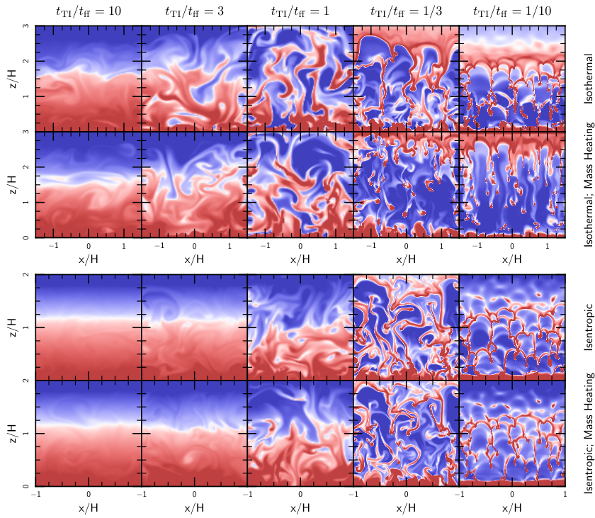
We extend our analysis into the non-linear regime using the numerical setup described in section 3. We have run a large suite of 2d and 3d simulations, summarized in Table 1. We focus our analysis on the presence of multi-phase structure (§ 5.1) and on the accreted mass flux (§ 5.2), both of which can be compared with observations of groups and clusters.
Equation 19c shows that the growth rate of the thermal instability is a factor of 3 smaller in plasmas with heating per unit mass than in plasmas with heating per unit volume. More generally, the timescale depends on the uncertain parameter and cannot be directly applied to (or inferred from) observations. Nonetheless, it is convenient to use to normalize time when considering the physics of the thermal instability with different values of . We also use the cooling time when we compare our results with observations. These two timescales differ only by an uncertain factor of order unity.
5.1 Multi-phase Structure
We performed simulations with the ratio of time-scales ranging from 0.1 to 10 (measured at ) and ran each for ten growth times, until . Fig. 1 shows representative snapshots of the density at the end of our fiducial simulations with volumetric heating and isothermal initial conditions. Our simulations show that plasmas with cooling times shorter than the dynamical time () develop spatially extended multi-phase structure, whereas plasmas with cooling times longer than the dynamical time () do not. Thus, the ratio controls the non-linear saturation of the thermal instability in stratified plasmas; this observationally-testable prediction is the primary result of our study. This conclusion does not depend strongly on either the initial stratification of the plasma or on our choice of heating per unit volume. To demonstrate this, Fig. 2 shows variations of our fiducial simulations with isentropic initial conditions and with mass-weighted heating. In all four cases, the saturated state transitions from single-phase to multi-phase when the ratio of time-scales becomes less than one. Below, we describe the plasma properties in these two limits and the physics of the transition between them.
The evolution of plasmas with short cooling times is straightforward: in this limit, the thermal instability develops and saturates before the plasma can buoyantly respond. The initial perturbations therefore collapse into dense clumps essentially in-situ, and the icm develops a highly inhomogeneous, multi-phase structure wherever . The clumps of cold gas then rain down onto the central galaxy on the (much longer) free-fall time, while bubbles of heated gas rise outwards. The rightmost panels of Figs. 1 and 2 illustrate this behavior. The result is a hotter atmosphere (in which ), filled with clumps of cold gas. We show in 64 that this end state resembles the observed properties of some cool-core groups and clusters.
The saturation of the thermal instability is fundamentally different when the cooling time is long compared to the dynamical time. In this limit, gravity and buoyancy influence the linear evolution of the perturbations (though the growth rate changes only by a factor of two). Nonlinearly, however, buoyancy provides a critical saturation channel for the thermal instability that prevents the formation of multi-phase gas. This conclusion is qualitatively similar to that reached by Balbus & Soker (1989); however, the physics is very different in our case because the background atmosphere remains statistically in thermal equilibrium for many cooling timescales. As initial perturbations cool and grow, they sink in the gravitational potential and mix with gas at lower radii. The cooling thus drives a slow, inward flow of material; the associated mass flux is, however, significantly smaller than is predicted by models without heating. We return to this point in the following sections. Rather than creating strong density inhomogeneities, cooling in this limit excites internal gravity waves with an amplitude that depends on the timescale ratio . These waves represent the overstability highlighted by Balbus & Soker (1989) and by Binney et al. (2009); we discuss their saturation below.
Our results depend crucially on the existence of a globally-stabilizing heating mechanism; if heating were not present, the atmospheres shown in Figs. 1 and 2 would collapse monolithically. This globally unstable case has been studied extensively by Balbus & Soker (1989). Consistent with their analysis, we find that atmospheres with small initial density inhomogeneities do not form multi-phase gas, regardless of (see 64 for a more detailed discussion).
Figs. 1 and 2 show that, assuming the existence of a globally stabilizing heating mechanism, plasmas with short cooling times develop spatially extended multi-phase structure, while plasmas with long cooling times do not. The left panel of Fig. 3 demonstrates this result more quantitatively. Here, we plot the mass fraction of cold gas (with ) at late times in the plane as a function of . (Recall that, in our units, .) This figure shows that the fraction of cold gas drops precipitously around and that there is essentially no multi-phase gas at large radii in simulations with .
The right panel of Fig. 3 quantifies the dependence of the saturated density fluctuations on the time-scale ratio and hints at the physics of the transition between the two limits. Here, we plot the root-mean-square (rms) average of the density perturbations
| (20) |
as a function of in the plane as in equation 3, indicates a spatial average at a given radius. In the short cooling time limit, the plasma develops multi-phase structure with large density perturbations . By contrast, in the long cooling time limit, the density perturbations saturate at much lower values . For plasmas with stable background stratification (e. g. our isothermal initial conditions), in this limit represents the amplitude of the gravity waves driven by cooling. Note that, while the mass fraction of cold gas drops off sharply around , Fig. 3 shows that the mean density fluctuation is a smooth function of this parameter, even in the weak cooling limit. We work to understand this quantitatively in section 6.
We emphasize that the difference in the evolution of plasmas with long and short cooling times does not simply result from the thermal instability taking longer to develop in simulations with weak cooling. We have run each simulation for a fixed number of growth times and, if gravity were not present, the results of our simulations with rapid and slow cooling would be nearly identical (we have confirmed this numerically). In fact, even in our simulations with long cooling times, the density contrast becomes large near the center of the potential, where gravity is weak (eq. 8) and the thermal instability has time to develop. The development of multi-phase structure depends on both gravity and cooling and therefore on the parameter , rather than simply on the cooling time alone.
5.2 Accreted Mass Flux
Fig. 4 shows the instantaneous, mean mass flux through the plane as a function of time in three of our 3d, fiducial simulations. The mass fluxes are normalized to the values predicted by cooling-flow models without heating, . It is clear that the mass flux is strongly suppressed relative to the cooling-flow solution whenever . This is not a trivial consequence of our feedback heating mechanism, because for , approaches . Rather, the suppression of for is also due to the non-linear saturation of the thermal instability (described below). The mass fluxes we find for are of the cooling-flow estimates and are therefore reasonably consistent with observational limits for cooling in the icm (Peterson & Fabian 2006). In 64 we show that this suppression is even stronger in spherical potentials and we explore its dependence on the details of our heating model.
In the rapid cooling limit, we find that gas heated at small radii, where the cooling time is shorter, rises up through the plane and initially drives an outflow. As the thermal instability progresses, however, this outflow reverses and a strong accretion flow develops (although the accreted material is all in the cold phase, rather than the hot phase; see the left panel of Fig. 3). The accretion rate approaches the cooling-flow value and eventually depletes the atmosphere of its gas. Thus, even our idealized feedback model (eq. 4) cannot suppress a cooling catastrophe when . We discuss the implications of this result in section 8 and, more thoroughly, in 64.
Fig. 4 is only meant to be suggestive, as several subtleties in our analysis complicate a precise interpretation of the accreted mass flux. For instance, we use only the initial value , though this quantity changes dramatically over the course of some of our simulations. Additionally, in simulations with , a more appropriate normalization for the mass flux might be , since the gas is not likely to flow in faster than its free-fall rate. 64 presents a much more realistic and thorough analysis of mass accretion rates.
5.3 Resolution Study
We test the numerical convergence of our results with 2d calculations on grids of resolution and for the full range of . Additionally, we performed 3d calculations of resolution and for atmospheres with , , and . Fig. 5 shows the distribution of density perturbations in our 2d simulations; this quantity has no apparent trend with resolution. Similarly, our 3d simulations are nearly identical at resolutions of and . Though Fig. 5 only demonstrates convergence of an integrated quantity, our simulations also “look” very similar at different resolution: for example, in the rapid-cooling limit, the clumps of cold gas have similar shapes and sizes, and they appear in the same locations.
We find rapid convergence in our simulations, even without including thermal conduction. By contrast, Sharma et al. (2010) found that convergence requires resolving the Field length (§ 7.2) in the cold phase of the icm. The temperature floor we apply (eq. 6) implies that the Field length is not defined for the cold phase in our simulations, and therefore that it is not relevant for convergence. Because the cold phase in our simulations does not cool, it can become pressure-supported at a finite size and resist further collapse. Convergence is somewhat less restrictive in our simulations than in those studied by Sharma et al. (2010).
We performed both 2d and 3d simulations and have confirmed that they give similar results. Many of the plots in this paper show the results of 2d simulations, since they are less expensive and permit a much larger parameter study. Because 2d simulations contain fewer grid cells than 3d simulations, however, integrated quantities derived from 2d calculations are noisier. Thus, we chose to include only 3d simulations in Figs. 4 and 8.
While our 2d and 3d simulations produce similar results, they are fundamentally different from one-dimensional simulations. Spatial variations between heating and cooling drive the local thermal instability in our model; hence, the development of multi-phase structure in our simulations is an inherently multi-dimensional effect. Additionally, the symmetry of a one-dimensional model prevents over-dense material from sinking and removes an important saturation channel from the thermal instability (§ 6). Much of the physics we describe in this paper is therefore absent in one-dimensional treatments of the icm such as those described in Ciotti & Ostriker (2001) and Guo & Oh (2008).
5.4 Sensitivity to the Heating Function

An important test of our model is the sensitivity of our conclusions to the details of the (unknown) heating function. We study this dependence by adding random heating fluctuations of the form
| (21) |
where is a Gaussian-random field with a white-noise spatial power spectrum and a temporal autocorrelation function . Thus, introduces both spatial and temporal imbalances between heating and cooling, which persist for the coherence time . These fluctuations detune our feedback model while still preserving average thermal equilibrium, and are intended to mimic the temporal and spatial differences between heating and cooling which might arise in a more realistic feedback scenario. More importantly, including these fluctuations allows us to distinguish between results that are a consequence of the exact (and, in detail, unphysical) balance in equation 4 and results that are more robust and are primarily a consequence of global thermal stability.
We carried out 2d simulations with , , and with the fluctuations normalized to root-mean-square (rms) amplitudes of 50%, 100% and 300%. (Note that we quote the rms, or ‘1’ amplitude of the fluctuations; the peak values are considerably higher.) Fig. 6 shows images of the density fluctuations for these simulations and Fig. 7 shows the temperature distribution function for different values of and the fluctuation amplitude. These figures demonstrate that our conclusions about the development of the thermal instability are essentially unaffected by order-unity fluctuations, over at least 10 cooling times. This important result implies that, as long as the plasma is in approximate global thermal equilibrium on reasonable time-scales and length-scales , the development and saturation of local thermal instability will proceed approximately as shown in Figs. 1–4. We think that the existence of an approximate thermal equilibrium, rather than the specific details of our heating function (eq. 4), determines how the thermal instability develops and saturates. This conclusion is bolstered by 64, which finds very similar results using an entirely different heating function.
Figs 6 and 7 show that extremely strong heating fluctuations with rms amplitudes of 300% spoil the thermal equilibrium of the plasma and induce a cooling catastrophe; even our extremely optimistic feedback model cannot withstand arbitrarily large heating perturbations. Though the feedback mechanism is not yet understood in clusters, this places a constraint on the heating: it should not differ persistently from the local cooling rate by more than a factor of several. Fig. 7 shows that this conclusion is essentially independent of the coherence time of the heating.
6 Interpretation of the Non-Linear Saturation
In this section, we show that the linearized dynamical equations provide valuable insight into the non-linear saturation of the thermal instability and its astrophysical implications. As in section 5, we focus on the development of multi-phase structure (§ 6.2) and on the accreted mass flux (§ 6.3), which have been extensively studied observationally. Our basic procedure is to estimate a saturation amplitude for the linear instability. Because we use linearized equations, the interpretation in this section only strictly holds in the weak cooling limit (), so that the density perturbations remain relatively small.
Fig. 8 illustrates the development and saturation of the thermal instability. The density inhomogeneity (or any other quantity linear in the perturbation) initially grows exponentially according to the dispersion relation (eq. 16), but eventually freezes out at a finite amplitude. This amplitude, along with the relations 12a–12c, then approximately determines the state of the plasma at late times. In the following sections, we estimate this amplitude and show that we can reproduce elements of the non-linear saturation shown in Fig. 3. Fig. 8 shows that the difference between atmospheres which develop multi-phase gas and ones which do not is fundamentally a non-linear effect. The linear growth rate of the perturbations is largely independent of the time-scale ratio , and it is the saturation which determines the degree of inhomogeneity at late times.
6.1 Saturation Amplitudes
In the limit that the plasma is buoyantly neutral (), we can estimate the saturation amplitude by inspecting the linearized, Lagrangian form of the momentum equation (eq. 1b):
| (22) |
The characteristic inflow (or outflow) time for a perturbed fluid element is . Initially, is small and this inflow time is long compared to the growth time of the thermal instability. As the perturbation grows, however, increases and the fluid element accelerates according to equation 22. The inflow time thus becomes shorter as the instability develops. We assume that the growth ceases when the inflow time is comparable to, or slightly shorter than, the growth time of the thermal instability. In this case, the thermal instability saturates when the velocity satisfies
| (23) |
Thus, non-linear saturation occurs when a fluid element flows to smaller radii after one cooling time, as seems intuitively reasonable.
The physical picture of a sinking fluid element does not apply in a stably stratified atmosphere, since the fluid element does not flow monotonically inwards, but instead oscillates with the gravity wave frequency . The velocity associated with this oscillation dwarfs the mean, inward velocity. These waves are sourced by cooling, however, and we assume that they reach a steady-state in which the dissipation rate due to non-linear mode coupling equals the driving rate due to the thermal instability . Thus the instability saturates when the dissipation time , where we have assumed strong turbulence and used the fact that the waves are driven on large scales, (as suggested by the bottom panels in Fig. 1). Though this saturation mechanism is very different from that described above for buoyantly neutral plasmas, it implies an equivalent saturation amplitude. We therefore assume that equation 23 describes the late-time evolution of the perturbations in all of our simulations. We show in the following sections how the behavior described in section 5 can be understood in terms of this saturation amplitude.
6.2 Multi-Phase Structure
Inserting our ansatz for the saturation amplitudes (equation 23) into the momentum equation (12b) and using the dispersion relation (equation 16) to replace , we express the density inhomogeneity at late times in terms of other properties of the plasma:
| (24) |
where and is the squared horizontal component of the direction of the wave vector (typically ).
Equation 24 has the asymptotic forms
| (25a) | |||||
| (25b) | |||||
Equation 25 shows that weakly stratified plasmas with develop smaller density inhomogeneities than plasmas with (in the limit that ). This difference arises because because plasmas with can sustain internal gravity waves, while atmospheres with cannot.
Somewhat surprisingly, the right panel of Fig. 3 shows that the measured dependence of on the time-scale ratio is in good agreement with equation 25b for both isothermal and isentropic initial conditions, even though in an isentropic atmosphere. This is because equation 25a applies only when the atmosphere is very nearly buoyantly neutral (at least when is long compared to the dynamical time, as must be for equation 25 to be valid). While this is the case initially in our isentropic atmospheres, the entropy gradient evolves somewhat with time and equation 25a ceases to describe the plasma after only a few cooling times. The saturated values of differ in our simulations with isentropic and isothermal initial conditions; equation 25b suggests that this may explain the systematic offset between these simulations shown in Fig. 3. For the longest cooling times, the evolution of the background profile is smallest; the slight steepening of for our isentropic simulations in this limit may represent an intermediate case between equations 25a and 25b.
6.3 Accreted Mass Flux
We can also use our estimate of the non-linear saturation to understand the inward mass flux induced by the thermal instability. Defining the mass flux and using the estimates of and from the momentum equation and from equation 24, we find
| (26) | ||||
where is the mass flux expected in the absence of heating (recall that we are in the limit that ). This yields
| (27) |
Equation 27 shows that the mass flux is dramatically suppressed when , qualitatively consistent with Fig. 4. Furthermore, this suppression is nearly independent of the initial stratification of the plasma, even though stably stratified plasmas show much stronger density inhomogeneities (eq. 25). This is because the internal gravity waves that enhance when do not contribute to the net mass flux. Note that gravity waves dominate the instantaneous mass flux shown in Fig. 4 when ; the time-averaged accretion rate is smaller than the figure suggests.
7 Simulations Including Conduction and Magnetic Fields

The previous sections describe a simplified model of the thermal instability that neglects both conduction and the dynamical effect of the magnetic field. This model nicely isolates the physics of the thermal instability, but astrophysically it is too idealized. For example, conduction is critical for the thermal evolution of the plasma over a wide range of scales in the icm, and Balbus (2000) and Quataert (2008) have shown that this completely changes the stability and dynamics of the plasma. In this section, we present results including magnetic fields and conduction and show that the conclusions from the previous sections largely apply in this more realistic case.
7.1 Setup
Our setup is very similar to that described in sections 2 and 3. We generalize equations 1b and 1c to include the effects of thermal conduction and the magnetic field:
| (1b′) | |||
| (1c′) |
where is the magnetic field and is the conductive heat flux. We evolve the magnetic field using the induction equation:
| (1d′) |
We have ignored both (explicit) viscous and magnetic dissipation in equations ′ ‣ 7.1–1d′. These effects can influence mhd simulations in subtle and unexpected ways (Fromang & Papaloizou 2007; Davis et al. 2010, see, e. g.), and so will need to be studied in detail in the future.
The thermal conductivity of the plasma is strongly anisotropic in the icm and as a result the conductive heat flux is given by (Braginskii 1965)
| (28) |
where is a unit vector in the direction of the magnetic field and is the thermal diffusivity of free electrons (with units of cm2/s). While the diffusivity depends sensitively on temperature (Spitzer 1962), we take it to be constant in this exploratory analysis. This enables us to control the ratio of the conduction time to other timescales in the problem and thus to isolate the physics of cooling and conduction. Note that we still use the heating function defined by equation 4; any conductive heating or cooling of the plasma happens on top of the feedback heating.
We initialize the plasma with a weak, horizontal magnetic field. (By ‘weak,’ we mean that magnetic tension is negligible in our simulations.) Because we impose reflecting boundary conditions at the upper and lower boundaries of the domain (§ 3), the magnetic field remains horizontal there and prohibits a conductive heat flux into the domain.
As before, we solve equations 1a and ′ ‣ 7.1–1d′ using Athena with the modifications described in section 3. We also implement equation 28 via operator splitting, using the anisotropic conduction algorithm described in Parrish & Stone (2005) and Sharma & Hammett (2007). In particular, we use the monotonized central difference limiter on transverse heat fluxes to ensure stability. This conduction algorithm is sub-cycled with respect to the main integrator with a time step ; these simulations are therefore more computationally expensive than adiabatic mhd calculations, especially at high resolution.
7.2 Linear Properties
We linearize equations 1a and ′ ‣ 7.1–1d′ and perform a WKB analysis (see Quataert 2008 for more details). Assuming that magnetic tension is negligible, and proceeding as in section 4.1, the dispersion relation for the plasma is (Balbus & Reynolds 2010, cf.)
| (29) |
In the above, is the growth rate of the perturbation, is the growth rate of the thermal instability accounting for conduction (Field 1965),
| (30) |
is inversely proportional to the conduction time across the wavelength of the perturbation, and
| (31) |
is the growth rate of either the magnetothermal instability (Balbus 2000, mti;), or the heat-flux driven buoyancy instability (Quataert 2008, hbi;).
The mti is unlikely to influence the development of multi-phase structure in galaxy clusters, since it operates outside the cool core, where the ratio of timescales is typically much greater than unity. While the hbi does operate efficiently in cool cores, it behaves like ordinary stable stratification in its saturated state (McCourt et al. 2011) and the growth time is analogous to the timescale used earlier. Thus, we do not expect the hbi or mti to change our results in any essential way (although this must be studied more carefully in future work). We anticipate that the same will be true for the overstabilities associated with the mti and hbi (Balbus & Reynolds 2010). In this section, we use simulations with isothermal initial conditions (in which ) so that these instabilities and overstabilities do not operate (at least in our initial conditions). This allows us to focus on the physics of thermal instability.
The conduction frequency is a function of scale, while the growth rate of the thermal instability is not; the modified growth rate therefore must switch sign at the length-scale
| (32) |
known as the Field length (Field 1965). Intuitively, the Field length is the distance heat can diffuse in one cooling time; if the wavelength of a perturbation is larger than this distance, conduction cannot stabilize it against cooling and the perturbation grows exponentially.
Conduction suppresses the thermal instability on scales smaller than the Field length, but the Field length in a magnetized medium depends on direction, as well as position. Even if the term in square brackets in equation 32 becomes arbitrarily large, the Field length will be small in directions orthogonal to the magnetic field. Because of this anisotropy, the thermal instability can still grow on scales much smaller than . Sharma et al. (2010) have studied this growth in the absence of gravity; here we generalize their results to stratified plasmas.
The growth rate for the thermal instability in our simulations is
| (33a) | ||||
| (33b) | ||||
Equation 33 shows that the characteristic growth time of the thermal instability is , regardless of the entropy gradient. The growth rate reduces to on large scales; thus, our results with and without conduction are very similar on scales larger than the Field length. Conduction prevents perturbations from growing below the Field length and therefore plays a similar role to the temperature floor in our non-conducting simulations. The primary difference between our conducting and non-conducting simulations is that the Field length is anisotropic in the conducting simulations, and the thermally unstable fluid elements collapse into long filaments, rather than the approximately spherical clumps shown in Figs. 1 and 2.
7.3 Numerical Results
Fig. 9 shows 2d slices of 3d simulations with different values of the cooling constant and the conductivity . We use only 3d simulations in this section because, just as an over-dense fluid element cannot sink in one dimension, the dynamics of a sinking magnetized filament changes in going from two to three dimensions. These simulations all use our isothermal initial condition and initially have weak, horizontal magnetic field lines in the plane of the figure. Rapid conduction smears out the cold clumps into filaments of length , but does not otherwise alter the growth of the thermal instability. Specifically, Fig. 9 demonstrates that, even in the limit of very rapid conduction, the ratio of time-scales determines whether the plasma develops multi-phase structure. This result depends critically on the anisotropic nature of thermal conduction. In the rightmost panels of Fig. 9, the Field length is larger than the entire simulation domain; if conduction were isotropic, the entire atmosphere would become nearly isothermal and the thermal instability would be suppressed. The insulating effect of the magnetic field permits large temperature gradients orthogonal to the magnetic field and thus the formation of multi-phase structure (Sharma et al. 2010).
Fig. 10 quantifies the effect of conduction on the thermal instability: we show the mass fraction of cold gas (as in the left panel of Fig. 3) for 3d simulations with different thermal conductivities. In simulations with anisotropic thermal conduction, this mass fraction is almost independent of the conductivity, and it appears to converge in the limit that the conductivity becomes large. This behavior is consistent with Fig. 9. Together, these results imply that anisotropic conduction alters the morphology of the gas in the cold phase, but not the presence, absence, or amount of multi-phase structure.
We have also run a number of simulations with isotropic thermal conduction. These simulations use the same setup as before, but with the conductive heat flux , where (as before) is a constant, free parameter. In order to prevent conduction from changing the total energy content of the plasma, we set at the upper and lower boundaries of the computational domain so that there is no conductive heat flux into the domain. Fig. 10 shows that, while anisotropic conduction does not strongly influence the amount of cold gas produced by the thermal instability, isotropic conduction can quench it entirely: we see no multi-phase structure in our simulations with isotropic conduction whenever the Field length is comparable to, or larger than, the pressure scale-height. These conclusions also apply to other properties of the plasma quantified in section 5, e. g. the accreted mass flux: anisotropic thermal conduction has little effect on this quantity, while isotropic thermal conduction can strongly suppress it.
Voit et al. (2008) suggested that thermal instability produces multi-phase gas in clusters when the Field length is comparable to, or smaller than, the size of the cool core, but that conduction suppresses the formation of multi-phase structure for larger Field lengths. Coincidentally, in typical cool-core clusters, this criterion is quantitatively similar to our criterion on the ratio .33 3 This comparison makes use of the result from 64 that the threshold for multi-phase gas in spherical systems is closer to . However, because the icm is magnetized, thermal conduction is extremely anisotropic; the results of this section demonstrate that even very rapid thermal conduction cannot suppress local thermal instability. Thermal conduction only stabilizes modes parallel to the magnetic field, and multi-phase structure continues to develop via perturbations that are roughly orthogonal to the local magnetic field.
8 Discussion
| Extended | No Extended |
|---|---|
| Abell 133 | Abell 85 |
| Abell 478 | Abell 644 |
| Abell 496 | Abell 744 |
| Abell 780 | Abell 1650 |
| Abell 1795 | Abell 2029 |
| Abell 1991 | Abell 2142 |
| Abell 2597 | Abell 4059 |
| Sersic 159-03 | |
| Centaurus |
We use the surveys of McDonald et al. (2010); McDonald et al. (2011a); McDonald et al. (2011b) to determine whether a cluster shows multi-phase gas, and we use the data in the accept catalog to estimate for the hot icm. Our label ‘extended ’ signifies that the emission can be resolved and is known to exist outside the bcg; these are the Type I systems from McDonald et al.
Observational limits from x-ray spectroscopy (Peterson & Fabian 2006) and from the shape of the galaxy luminosity function (Benson et al. 2003) indicate that the diffuse plasma in galaxy groups and clusters does not cool as quickly as it radiates. These observations imply that some heating process offsets radiative cooling and that the gas remains in approximate thermal equilibrium, at least when averaged over length-scales comparable to the scale-height or time-scales comparable to the cooling time. The nature of this “feedback” heating is not yet fully understood, although it appears to involve heating by a central agn (Bîrzan et al. 2004; McNamara & Nulsen 2007, e. g.). More fully understanding the mechanism(s) that regulate the heating to so closely match cooling remains a major challenge in theories of galaxy formation.
Though heating strongly suppresses cooling in galaxy groups and clusters, star formation and multi-phase gas provide clear evidence for cold gas in many cluster cores. Observational indicators of this cold gas strongly correlate with the cooling time of the ambient hot icm (Voit et al. 2008; Rafferty et al. 2008; Cavagnolo et al. 2008; Cavagnolo et al. 2009, e. g.), motivating a model in which thermal instability in the hot icm produces much of the cold gas in cluster cores (as has been suggested many times in the past, e. g. Fabian & Nulsen 1977; Cowie et al. 1980; Nulsen 1986; Loewenstein et al. 1991). Theoretically studying local thermal instability in the icm has proven difficult, however, because of the cooling-flow problem: studies that include both cooling and gravity typically find that the plasma is globally thermally unstable, and that the entire cluster core collapses monolithically. This difficulty has led several authors to conclude that the thermal instability does not produce multi-phase structure in stably-stratified systems at all.
We avoid the cooling-flow problem in this paper by adopting a phenomenological heating model that enforces thermal equilibrium when averaged over large scales (§ 2.1). Our heating model is approximate, over-simplified, and wrong in detail. However, our results are insensitive to large temporal and spatial fluctuations about the average heating (§ 5.4). Moreover, in 64 we obtain similar results using a more physical feedback heating prescription. We therefore believe that our conclusions about the saturation of the local thermal instability are reasonably robust.
In the current paradigm in which clusters are approximately in global thermal equilibrium, heating of the icm is very likely to depend explicitly on position in the cluster. In this case, the thermal stability of the plasma is independent of its convective stability (§ 4.2). Fundamentally, buoyancy drives convection, while heating and cooling drive thermal instability. These two processes are formally related only under the restrictive assumption that heating is a state function of the plasma; more generally, they are unrelated and the thermal stability of a plasma is independent of its convective stability (Balbus & Soker 1989, see).
Nonetheless, it remains true that the competition between buoyancy and thermal instability determines the net effect of cooling on a stratified plasma. We parametrize the relative importance of these effects using the dimensionless ratio (the ratio of the thermal instability growth time to the local dynamical, or free-fall, time ). When this ratio is small, thermal instability dominates and the plasma develops significant multi-phase structure; when the ratio is large, buoyancy dominates and the plasma remains in a single, hot phase (§ 5). This dependence of the saturation on is true for both stably stratified and neutrally stratified plasmas (Fig. 3), even though the effect of buoyancy is very different in these two cases.
More quantitatively, we find (Fig. 3) that the saturated density inhomogeneities produced by the thermal instability approximately obey the relation
| (34) |
this scaling can be understood analytically by assuming a saturation amplitude for the thermal instability in which the characteristic fluid velocities approach (§ 6). Thus, by assuming that some heating mechanism prevents cooling catastrophes in clusters, we find that the icm breaks up into multiple phases via local thermal instability (with ) only if the dimensionless ratio of timescales ; specifically, there is almost no cold gas at large radii when (Fig. 3). This finding is one of the primary results of our analysis. We note that the linear growth of the thermal instability is largely independent of the ratio . Thus the difference between atmospheres which develop multi-phase gas and those which do not is fundamentally due to how the non-linear saturation of the thermal instability depends on the atmosphere’s properties.
The calculations in 64 show that the criterion for multi-phase structure is actually somewhat less stringent in spherical systems, . This difference stems from the fact that fluid elements are compressed as they move inwards in a spherical system; this compression enhances the density perturbations and accelerates the growth of the thermal instability.
Our criterion for multi-phase structure is not sensitive to large variations about our idealized heating prescription (§ 5.4 and Fig. 6). Furthermore, the multi-phase structure that develops via thermal instability is largely independent of the magnitude of the thermal conduction, even on scales much smaller than the Field length (provided conduction is anisotropic, as is the case in galaxy groups and clusters; § 7). Anisotropic thermal conduction changes the morphology of the cold gas produced via thermal instability (blobs filaments), but not the presence or amount of cold gas. There is thus a very strong, qualitative difference between isotropic and anisotropic thermal conduction (Fig. 10), which cannot be captured by simply multiplying the heat flux by a suppression factor (as is often done, e. g. Zakamska & Narayan 2003; Voit et al. 2008; Guo & Oh 2008).
Our heating prescription imposes global thermal equilibrium and reduces the accreted mass flux in our model halos relative to cooling-flow values. This reduction is not inevitable, however, because thermal instability can produce cooling-flow-like inflow rates when . In a globally stable system, the thermal instability thus plays an important role in regulating gas inflow rates. We study the connections among thermal instability, mass inflow and feedback more fully in 64.
We argue that a locally stable heating mechanism (such as the one proposed in Kunz et al. 2011) is not required to explain the reduced star formation and cooling rates in clusters. Instead, global stability arising from approximate thermal equilibrium, together with the physics of local thermal instability in stratified plasmas, is sufficient to reproduce the low net cooling rates in clusters. Moreover, the correlation of filaments and star formation in clusters with the cooling time in the hot icm strongly suggests that the plasma is in fact locally thermally unstable. We have shown that the suppression of accretion rates is not sensitive to thermal conduction or to significant variations about our specific feedback prescription (§ 5.4 and Fig. 6), and we explore this further in 64.
We now compare our model predictions with observational results. The thermal instability time (eq. 19) depends on the unknown way in which feedback energy is thermalized (eq. 4) and cannot be directly inferred from observations. We therefore use the cooling time when comparing our results with observations. These two timescales differ by an unknown factor of order unity. The ratio of timescales can be reexpressed in more familiar terms using
| (35) |
where is a measure of the plasma entropy, is the temperature in units of and is the cooling function (eq. 5) in units of . Thus, the plasma in clusters and galactic halos should show extended multi-phase structure wherever
| (36) |
where we have used the threshold from 64 for multi-phase structure in spherical systems: . This criterion is consistent with observations that clusters with central entropies below preferentially show signs of cold gas such as star formation and emission (Voit et al. 2008; Cavagnolo et al. 2008; Cavagnolo et al. 2009). Note, however, the relatively strong dependence of this criterion on and on ; this is because the entropy is not the fundamental parameter governing the saturation of the thermal instability in a stratified system.
The survey conducted by McDonald et al. (2010); McDonald et al. (2011a) permits another test of our criterion. McDonald et al. provide lists of groups and clusters with and without extended emission. We test our criterion by estimating the time-scale ratio for these systems using data from the accept catalog (Cavagnolo et al. 2009). We fit the entropy profiles of clusters in the accept catalog using and we fit the pressure profiles using the form provided in Arnaud et al. (2010). Of the groups and clusters in both the surveys and in accept, sixteen give reasonable fits (listed in Table 2).44 4 Unfortunately, we were unable to fit several clusters with well-known filament systems, including Perseus, Abell 2052 and M87. The pressure gradients in Perseus and Abell 2052 are positive at some radii and cannot be fit by the universal profile. Similarly, the pressure profile for M87 deviates from the broken power-law universal profile. From our fits to and , we calculate and and estimate using the fit to the cooling function provided by Tozzi & Norman (2001) with solar metallicity. We estimate from the pressure and density profiles by assuming spherical symmetry and hydrostatic equilibrium; from this we calculate .
The left panel of Fig. 11 shows as a function of radius for these sixteen groups and clusters. As predicted by our analysis, the clusters with short cooling times show extended filaments, while the clusters with long cooling times do not. Additionally, most of the filaments are found at radii around 10–50 kpc, where the ratio is the smallest. Although this evidence is not conclusive, these data support our hypothesis that the filaments condense from the icm due to the local thermal instability.
We emphasize that both cooling and gravity influence the development of the thermal instability in the icm. A short cooling time (or low ) is not sufficient for the formation of filaments; rather, the ratio is the relevant parameter. The right panel of Fig. 11 shows clusters in the ()–() plane. More data are needed to conclusively test our model, but these results are consistent with our interpretation that the ratio of timescales is a better predictor of multi-phase gas in hot halos than alone.
These simple comparisons support a model in which local thermal instability produces at least some of the filaments seen in clusters. This does not, however, imply that thermal instability alone can explain all of the observed properties of multi-phase gas in clusters and/or galaxies. On the contrary, processes such as conductive condensation of hot gas to cool gas (“non-radiative cooling;” Fabian et al. 2002; Soker et al. 2004) and the inflow of cold gas through the virial radius (Kereš & Hernquist 2009) may also be important (in higher and lower mass halos, respectively). Furthermore, other processes in the icm such as merger shocks, galaxy wakes and buoyant radio bubbles may influence the evolution of the filaments.
Accretion of the cold gas formed via thermal instability likely plays an important role in the evolution of brightest cluster galaxies and their central agn (Pizzolato & Soker 2005; Pizzolato & Soker 2010). In addition, the high-velocity clouds surrounding the Milky Way may also be manifestations of the thermal instability (Maller & Bullock 2004; Sommer-Larsen 2006; Kaufmann et al. 2006; Peek et al. 2008); this process could provide an important source of unenriched gas to maintain metallicity gradients (Jones et al. 2010) and continued star formation (Bauermeister et al. 2010) in the Milky Way and other galaxies.
Acknowledgments
We are grateful to Mark Voit and Megan Donahue for interesting and
helpful conversations as we completed this work, and to Steve Balbus for
clarifying our discussion of the previous literature. We thank the anonymous
referee for helping to clarify our discussion, particularly in
section 4. Mike McDonald helpfully suggested several
clusters we left out from Fig. 11 in an earlier version of this
paper. We are also thankful for the hospitality of the Kavli Institute for
Theoretical Physics (KITP) at UC Santa Barbara, where we performed some of
this work. KITP is supported in part by NSF grant number PHY-.
Support for P. S. was provided by NASA through Chandra Postdoctoral Fellowship
grant PF- awarded by the Chandra X-Ray Center, which is operated by
the Smithsonian Astrophysical Observatory for NASA under contract
NAS-. M. M., I. P. and E. Q. were supported in part by NASA Grant
NNXACG, NSF-DOE Grant PHY-, and by the David and Lucile
Packard Foundation. We performed many of the computations for this paper on
the Henyey cluster at UC Berkeley, supported by NSF AST Grant
; additional computing time was provided by the National Science
Foundation through the Teragrid resources located at the National Center for
Atmospheric Research under grant number TG-AST. We made our figures
using the open-source program Tioga. This research has made use of
NASA’s Astrophysics Data System.
References
- Arnaud et al. (2010) Arnaud, M., Pratt, G. W., Piffaretti, R., et al. 2010, Astronomy and Astrophysics, 517, A92
- Balbus (1986) Balbus, S. A. 1986, Astrophysical Journal Letters, 303, L79
- Balbus (1988) Balbus, S. A. 1988, Astrophysical Journal, 328, 395
- Balbus (2000) Balbus, S. A. 2000, Astrophysical Journal, 534, 420
- Balbus (2001) Balbus, S. A. 2001, Astrophysical Journal, 562, 909
- Balbus & Reynolds (2010) Balbus, S. A. & Reynolds, C. S. 2010, Astrophysical Journal Letters, 720, L97
- Balbus & Soker (1989) Balbus, S. A. & Soker, N. 1989, Astrophysical Journal, 341, 611
- Bauermeister et al. (2010) Bauermeister, A., Blitz, L., & Ma, C. 2010, Astrophysical Journal, 717, 323
- Benson et al. (2003) Benson, A. J., Bower, R. G., Frenk, C. S., et al. 2003, Astrophysical Journal, 599, 38
- Binney et al. (2009) Binney, J., Nipoti, C., & Fraternali, F. 2009, Monthly Notices of the Royal Astronomical Society, 397, 1804
- Bîrzan et al. (2004) Bîrzan, L., Rafferty, D. A., McNamara, B. R., Wise, M. W., & Nulsen, P. E. J. 2004, Astrophysical Journal, 607, 800
- Braginskii (1965) Braginskii, S. I. 1965, Reviews of Plasma Physics, 1, 205
- Cavagnolo et al. (2008) Cavagnolo, K. W., Donahue, M., Voit, G. M., & Sun, M. 2008, Astrophysical Journal Letters, 683, L107
- Cavagnolo et al. (2009) Cavagnolo, K. W., Donahue, M., Voit, G. M., & Sun, M. 2009, Astrophysical Journal Supplement, 182, 12
- Ciotti & Ostriker (2001) Ciotti, L. & Ostriker, J. P. 2001, Astrophysical Journal, 551, 131
- Cole et al. (2001) Cole, S., Norberg, P., Baugh, C. M., et al. 2001, Monthly Notices of the Royal Astronomical Society, 326, 255
- Cowie et al. (1980) Cowie, L. L., Fabian, A. C., & Nulsen, P. E. J. 1980, Monthly Notices of the Royal Astronomical Society, 191, 399
- Davis et al. (2010) Davis, S. W., Stone, J. M., & Pessah, M. E. 2010, Astrophysical Journal, 713, 52
- Defouw (1970) Defouw, R. J. 1970, Astrophysical Journal, 160, 659
- Fabian (1994) Fabian, A. C. 1994, Annual Reviews of Astronomy and Astrophysics, 32, 277
- Fabian et al. (2002) Fabian, A. C., Allen, S. W., Crawford, C. S., et al. 2002, Monthly Notices of the Royal Astronomical Society, 332, L50
- Fabian et al. (2008) Fabian, A. C., Johnstone, R. M., Sanders, J. S., et al. 2008, Nature, 454, 968
- Fabian & Nulsen (1977) Fabian, A. C. & Nulsen, P. E. J. 1977, Monthly Notices of the Royal Astronomical Society, 180, 479
- Fabian et al. (2003) Fabian, A. C., Sanders, J. S., Crawford, C. S., et al. 2003, Monthly Notices of the Royal Astronomical Society, 344, L48
- Ferland et al. (2009) Ferland, G. J., Fabian, A. C., Hatch, N. A., et al. 2009, Monthly Notices of the Royal Astronomical Society, 392, 1475
- Field (1965) Field, G. B. 1965, Astrophysical Journal, 142, 531
- Fromang & Papaloizou (2007) Fromang, S. & Papaloizou, J. 2007, Astronomy and Astrophysics, 476, 1113
- Guo & Oh (2008) Guo, F. & Oh, S. P. 2008, Monthly Notices of the Royal Astronomical Society, 384, 251
- Hattori & Habe (1990) Hattori, M. & Habe, A. 1990, Monthly Notices of the Royal Astronomical Society, 242, 399
- Heckman et al. (1989) Heckman, T. M., Baum, S. A., van Breugel, W. J. M., & McCarthy, P. 1989, Astrophysical Journal, 338, 48
- Holtzman et al. (1992) Holtzman, J. A., Faber, S. M., Shaya, E. J., et al. 1992, Astronomical Journal, 103, 691
- Hu et al. (1985) Hu, E. M., Cowie, L. L., & Wang, Z. 1985, Astrophysical Journal Supplement, 59, 447
- Jones et al. (2010) Jones, T., Ellis, R., Jullo, E., & Richard, J. 2010, Astrophysical Journal Letters, 725, L176
- Joung et al. (2011) Joung, M. R., Bryan, G. L., & Putman, M. E. 2011, ArXiv e-prints
- Kaufmann et al. (2006) Kaufmann, T., Mayer, L., Wadsley, J., Stadel, J., & Moore, B. 2006, Monthly Notices of the Royal Astronomical Society, 370, 1612
- Kereš & Hernquist (2009) Kereš, D. & Hernquist, L. 2009, Astrophysical Journal Letters, 700, L1
- Kochanek et al. (2001) Kochanek, C. S., Pahre, M. A., Falco, E. E., et al. 2001, Astrophysical Journal, 560, 566
- Kunz et al. (2011) Kunz, M. W., Schekochihin, A. A., Cowley, S. C., Binney, J. J., & Sanders, J. S. 2011, Monthly Notices of the Royal Astronomical Society, 410, 2446
- Loewenstein et al. (1991) Loewenstein, M., Zweibel, E. G., & Begelman, M. C. 1991, Astrophysical Journal, 377, 392
- Lynds & Sandage (1963) Lynds, C. R. & Sandage, A. R. 1963, Astrophysical Journal, 137, 1005
- Lynds (1970) Lynds, R. 1970, Astrophysical Journal Letters, 159, L151
- Malagoli et al. (1987) Malagoli, A., Rosner, R., & Bodo, G. 1987, Astrophysical Journal, 319, 632
- Malagoli et al. (1990) Malagoli, A., Rosner, R., & Fryxell, B. 1990, Monthly Notices of the Royal Astronomical Society, 247, 367
- Maller & Bullock (2004) Maller, A. H. & Bullock, J. S. 2004, Monthly Notices of the Royal Astronomical Society, 355, 694
- McCarthy et al. (2004) McCarthy, I. G., Balogh, M. L., Babul, A., Poole, G. B., & Horner, D. J. 2004, Astrophysical Journal, 613, 811
- McCourt et al. (2011) McCourt, M., Parrish, I. J., Sharma, P., & Quataert, E. 2011, Monthly Notices of the Royal Astronomical Society, 413, 1295
- McDonald et al. (2011a) McDonald, M., Veilleux, S., & Mushotzky, R. 2011a, Astrophysical Journal, 731, 33
- McDonald et al. (2010) McDonald, M., Veilleux, S., Rupke, D. S. N., & Mushotzky, R. 2010, Astrophysical Journal, 721, 1262
- McDonald et al. (2011b) McDonald, M., Veilleux, S., Rupke, D. S. N., Mushotzky, R., & Reynolds, C. 2011b, Astrophysical Journal, 734, 95
- McNamara & Nulsen (2007) McNamara, B. R. & Nulsen, P. E. J. 2007, Annual Reviews of Astronomy and Astrophysics, 45, 117
- Nulsen (1986) Nulsen, P. E. J. 1986, Monthly Notices of the Royal Astronomical Society, 221, 377
- O’Dea et al. (2010) O’Dea, K. P., Quillen, A. C., O’Dea, C. P., et al. 2010, Astrophysical Journal, 719, 1619
- Oh & Benson (2003) Oh, S. P. & Benson, A. J. 2003, Monthly Notices of the Royal Astronomical Society, 342, 664
- Parrish & Stone (2005) Parrish, I. J. & Stone, J. M. 2005, Astrophysical Journal, 633, 334
- Peek et al. (2008) Peek, J. E. G., Putman, M. E., & Sommer-Larsen, J. 2008, Astrophysical Journal, 674, 227
- Peterson & Fabian (2006) Peterson, J. R. & Fabian, A. C. 2006, Physics Reports, 427, 1
- Pizzolato & Soker (2005) Pizzolato, F. & Soker, N. 2005, Astrophysical Journal, 632, 821
- Pizzolato & Soker (2010) Pizzolato, F. & Soker, N. 2010, Monthly Notices of the Royal Astronomical Society, 408, 961
- Quataert (2008) Quataert, E. 2008, Astrophysical Journal, 673, 758
- Rafferty et al. (2008) Rafferty, D. A., McNamara, B. R., & Nulsen, P. E. J. 2008, Astrophysical Journal, 687, 899
- Rees & Ostriker (1977) Rees, M. J. & Ostriker, J. P. 1977, Monthly Notices of the Royal Astronomical Society, 179, 541
- Saro et al. (2006) Saro, A., Borgani, S., Tornatore, L., et al. 2006, Monthly Notices of the Royal Astronomical Society, 373, 397
- Sharma & Hammett (2007) Sharma, P. & Hammett, G. W. 2007, Journal of Computational Physics, 227, 123
- Sharma et al. (2012) Sharma, P., McCourt, M., Quataert, E., & Parrish, I. J. 2012, Monthly Notices of the Royal Astronomical Society, 420, 3174
- Sharma et al. (2010) Sharma, P., Parrish, I. J., & Quataert, E. 2010, Astrophysical Journal, 720, 652
- Sijacki & Springel (2006) Sijacki, D. & Springel, V. 2006, Monthly Notices of the Royal Astronomical Society, 366, 397
- Silk (1977) Silk, J. 1977, Astrophysical Journal, 211, 638
- Soker (2006) Soker, N. 2006, New Astronomy, 12, 38
- Soker et al. (2004) Soker, N., Blanton, E. L., & Sarazin, C. L. 2004, Astronomy and Astrophysics, 422, 445
- Sommer-Larsen (2006) Sommer-Larsen, J. 2006, Astrophysical Journal Letters, 644, L1
- Spitzer (1962) Spitzer, L. 1962, Physics of Fully Ionized Gases (New York: Interscience Publishers)
- Tozzi & Norman (2001) Tozzi, P. & Norman, C. 2001, Astrophysical Journal, 546, 63
- Voit et al. (2008) Voit, G. M., Cavagnolo, K. W., Donahue, M., et al. 2008, Astrophysical Journal Letters, 681, L5
- White & Rees (1978) White, S. D. M. & Rees, M. J. 1978, Monthly Notices of the Royal Astronomical Society, 183, 341
- Zakamska & Narayan (2003) Zakamska, N. L. & Narayan, R. 2003, Astrophysical Journal, 582, 162