Fine Features in the Primordial Power Spectrum
Abstract
A possible origin of the anomalous dip and bump in the primordial power spectrum, which are reconstructed from WMAP data corresponding to the multipole by using the inversion method, is investigated as a consequence of modification of scalar field dynamics in the inflation era. Utilizing an analytic formula to handle higher order corrections to the slow-roll approximation, we evaluate the relation between a detailed shape of inflaton potential and a fine structure in the primordial power spectrum. We conclude that it is unlikely to generate the observed dip and bump in the power spectrum by adding any features in the inflaton potential. Though we can make a fine enough shape in the power spectrum by controlling the feature of the potential, the amplitude of the dip and bump becomes too small in that case.
1 Introduction
Inflation has been the focus of attention as a successful scenario which gives not only a natural understanding of initial conditions of the standard Big Bang Cosmology, but also a generation mechanism of primordial curvature fluctuations, which eventually turn into Cosmic Microwave Background (CMB) anisotropies and Large Scale Structure of the universe. Current precise data of cosmological observations, e.g., Wilkinson Microwave Anisotropy Prove (WMAP) data [1], predict a nearly scale-invariant power spectrum of primordial curvature fluctuations. As is well-known, such kind of the power spectrum can be generated from the standard single slow-roll inflation. In keeping with the progress of the cosmological observations, however, small characteristic features in the primordial power spectrum, e.g., a lack of large-scale power, small dip and bump at multipole , a fine oscillating structure around multipole and so on[1, 2], have gotten more and more attention.
In fact, there are many attempts to explain such features in the primordial power spectrum by considering a non-trivial dynamics of the scalar field during inflation. For example, several authors[5, 4, 6] claimed that the small dip and bump at multipole can be explained due to the temporarily breaking off from the slow-roll dynamics of the inflaton field. They employed an inflaton potential with a sharp step proposed by Adams et al.[3]:
| (1) | |||||
| (2) |
Indeed, the above effective potential can be naturally considered in the two-field inflation model with a very small mass difference between two inflaton fields. Here the parameter characterizes the ”mass gap”. For the small value of , the general slow-roll approximation formula proposed by ref. [11] is applicable to the generation of primordial curvature fluctuations. Either employing this approximation or numerically solving the perturbation equations, the authors obtained a power spectrum of primordial curvature fluctuations which can explain the observed small dip and bump at in the CMB temperature power spectrum [5, 4, 6]. It should be noted that the width of an oscillation in the power spectrum of curvature fluctuations is approximately in order to match the WMAP data.
Recently, a new oscillating structure around multipole has been reported[7, 8]. The authors employed the inversion method to reconstruct the primordial curvature fluctuations from the WMAP data. The width of the structure they found in the primordial power spectrum is , which is much finer than the structure at . In order to realize such a fine structure in the primordial power spectrum, Nakashima et al.[9] have proposed a sudden change of the sound velocity during inflation induced by a non-canonical kinetic term of the inflaton. They found fine oscillations in the primordial power spectrum, while these oscillatory features continue on the scales smaller than the Hubble radius at the time of the sound velocity change. Therefore such a model may screw up the matching between the observational data and theoretical predictions at which corresponds to the scale of the first acoustic peak.
In this paper, we investigate other possibilities of generating the fine structure of the primordial power spectrum by modifying the inflaton potential. Employing the general slow-roll approximation formula, we can easily find the relation between the fine structure of the primordial power spectrum and the evolution of the slow-roll parameters during inflation. Here the dynamics of the inflaton determines the evolution of slow-roll parameters. For example, it can be shown that the mass transition which is described by eq.(2) modifies the monotonic evolution of the slow roll parameters and eventually generates a structure in the primordial power spectrum. We expect that the shorter the mass transition is, the finer the structure becomes.
This paper is organized as follows. In the next section, we briefly review and investigate an analytical formula to obtain the primordial power spectrum, that is, the general slow-roll formula. In section 3, based on the formula, we discuss the possibility of generating fine structures in the primordial power spectrum due to the modification of the monotonic evolution of the slow roll parameters. The last section is devoted to the summary and discussion.
2 General slow-roll formula
Let us consider a single canonical scalar field whose action is given by
| (3) |
where is a metric and represents the potential of the scalar field. The power spectrum of the curvature perturbation induced by quantum fluctuations of the scalar field can be defined as
| (4) |
In the standard single-field slow-roll inflation, the power spectrum is simply given by
| (5) |
where is the Hubble parameter, is the derivative of the inflaton with respect to the cosmic time and the subscript , with being a scale factor, denotes that the expression is to be evaluated at the time when the scale of interest exits the horizon. The above simple formula can be obtained under the assumptions that the slow-roll parameters are small and keep almost constant values in time. Even if the case these assumptions are violated, however, a general formula of the power spectrum of primordial curvature perturbations proposed by Stewart [11] can be applicable, which is refereed as the general slow-role formula. Following ref. [11], let us briefly review this formula.
The time evolution of can be described by [10]
| (6) |
where is a conformal time, and
| (7) |
Using the slow-roll parameters and , we have
| (8) |
where
| (9) |
It should be noted that Eq.(8) is applicable for any values of the slow roll parameters, while in the standard slow roll approximation, we assume that , and their time derivatives are also small.
As far as the slow-roll parameters are order of unity or less, we find . Hence, on the super-horizon scales (), the above evolution equation (6) can be approximately reduced as
| (10) |
From this equation, we can easily find that in the single field inflation the curvature perturbations , remain constant in time on the super-horizon scales. On the other hand, on the sub-horizon scales, namely , eq. (6) can be reduced as
| (11) |
This equation looks similar to the equation of motion for the harmonic oscillator in the Minkowski spacetime and hence the evolution of is decoupled from the background inflationary dynamics.
From the above discussion, the power spectrum of strongly depends on the inflationary dynamics around the horizon crossing time. Therefore, in order to have a specific feature in the power spectrum, the modification of slow-roll dynamics has to take place at the epoch of horizon crossing for the corresponding scale.
Now we are at the position to solve the eq.(6) by employing the general slow roll approximation. Let us first obtain the asymptotic solutions. On the super-horizon scales, stays constant in time as we have already shown. On the sub-horizon scale, we adopt the Bunch-Davies vacuum to provide initial conditions. Accordingly, we have the asymptotic solutions as
| (12) |
Following ref. [11], we introduce non-dimensional variables and . We also convert to as
| (13) |
Then equation of motion can be rewritten as
| (14) |
where the source function is defined as
| (15) |
Hence the power spectrum of the comoving curvature perturbation is given by
| (16) |
Since the asymptotic behavior of the homogeneous solution of eq. (14) has to match with the one of eq.(12), we obtain the homogeneous solution of eq. (14) as
| (17) |
Therefore, using the Green’s function method, we obtain the formal solution of eq. (14) as
| (18) |
Since can be written in terms of slow-roll parameters and their time derivatives as shown below, we can solve the above formal solution iteratively. In fact, under a slow-roll condition; , we can rewrite the conformal time as
| (19) |
By using this expression, the source function can be expressed as
| (20) | |||||
Unlike the standard slow-roll approximations, we take into account the time derivatives of the parameters, such as and in this general slow-roll formula.
Then, up to the first order in the source function , we develop an analytical formula of the power spectrum of the curvature perturbations as
| (21) |
where denotes the value at the horizon crossing time, , and the window function
| (22) |
with
| (23) | |||||
Figure 1 shows the form of the window function.
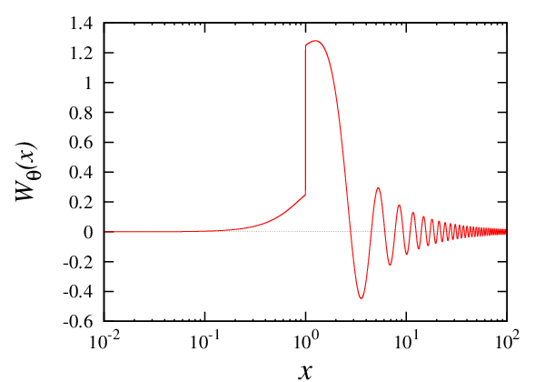
In this figure, since is the horizon crossing time for a given wavenumber, corresponds to the time after the horizon exit (on super-horizon scales) and while to the time before the horizon exit (on sub-horizon scales). This function reflects the behavior of the homogeneous solution . Due to the oscillatory behavior of the window function for and the sharp cut-off for coming from the step function, we can easily find that the integral term of the formula mostly depends on the behavior of the source function around the horizon cross time. Therefore it is clear that the specific feature on the power spectrum induced by the modification of slow-roll dynamics appears only at the scales crossing the horizon when the modification takes place.
If slow-roll conditions are satisfied, the source function and are approximately zero. Then, we verify that eq. (21) leads to the well-known slow-roll expression (5);
Therefore, we can conclude that eq. (21) is a natural extension of the slow-roll approximation to the generalized one. In appendix A, we check the validity of this general slow-roll formula.
3 Can we make fine structures in the primordial power spectrum?
In the previous section, we have briefly reviewed the general slow-roll formula to evaluate the primordial power spectrum in which we iteratively take into account the modification of the slow-roll dynamics. The analytical formula eq. (21) consists of the window function which reflects the behavior of the homogeneous solution , and the source function related to the inflationary background dynamics through the slow-roll parameters. Accordingly, the fine structures of the primordial power spectrum depends on the form of the window function and also that of the source function. In this section, using the analytical formula, we study the modification of the primordial power spectrum by considering the effect of the modification of the slow-roll dynamics. We focus on the relation between the fine structures of the primordial power spectrum and the form of the source function with keeping the form of the window function.
3.1 Source function
![[Uncaptioned image]](1105.2398v1/source_check.png)
![[Uncaptioned image]](1105.2398v1/width_compare.png)
|
First, let us briefly mention how the functional form of can be related with theoretical models of inflation. Stewart [11] has calculated the primordial power spectrum by making use of the general slow-roll formula with changing the functional form of . In this paper, however, we focus on the form of the source function instead of which we can construct from by using eq. (15).
In eq. (20), we gave the expression for with respect to the slow-roll parameters defined by eq. (9). Here, we give another expression for in terms of derivatives of potential such as and , time derivative of and Hubble parameter as
| (27) |
In order to investigate which term of the right hand side of this equation mainly contributes to , in figure 3 we show the source function and for a bump model whose potential is given by
| (28) |
From this figure, it is found that the form of is dominated by . We find that this is also true for the case of a step in the potential. Therefore we can conclude that controls when the dynamics of the inflaton modifies due to the fine structure in the potential. As is well known, represents the effective mass of the scalar field. In this sense, it is considered that the source function traces the change of the mass of the inflaton. Of course, if the inflaton is coupled with other massive scalar fields during inflation, then the effective mass of the inflaton can be affected by the evolution of such massive fields. Hence, such kind of fine structures in the primordial power spectrum may provide some clues for high energy physics [12, 15, 13, 14, 16, 17].
Let us now focus on the width of the source function which may control the width of the primordial power spectrum. On the contrary, the width of should relate with the one of the inflaton potential. Figure. 3 shows the relation of the to the parameter which is defined as the width of as is shown in figure 3. From this figure, it is clear that the width of is a monotonic function of the one of the inflaton potential. Hence, when we can find the form of the function through the observations of the primordial power spectrum, we can easily reconstruct the potential form of the inflaton. In the following discussion, we consider the effect of the anomalous structure of the inflaton potential on the primordial power spectrum with changing the functional form of .
Before closing this subsection, we would like to remark that we can separate into two components, namely the smooth part whose integration in terms of time produces a power law component in the primordial power spectrum and the gap part which corresponds to a fine structure in the spectrum as
| (29) |
Note that the function in eq. (21) can be derived by integrating the function from its definition eq. (15). Here the power law part can be written by using the spectral index , which is defined as , as
| (30) |
In this paper, we adopt [1].
On the other hand, we employ a general form of the inflaton potential with steps and bumps to investigate whether we can obtain the observed fine structure at or not in the next subsection. It turns out that the resultant functional form of can be described by the differential Gaussian function.
3.2 Fine structures of the power spectrum controlled by


|


|
In order to investigate the fine structure of the primordial power spectrum due to the modification of the slow-roll dynamics, we employ the differential Gaussian function as the gap part of the source function , given by
| (31) |
Here is the Gauss symbol. It should be noticed that and correspond to a step and a bump / dip in the inflaton potential, respectively. Therefore the differential Gaussian function for is a natural and general extension of the inflaton potential with simple fine features. Moreover, the width and height of the features can be easily controlled by changing the parameters and , respectively.
Our goal is to explain the newly found fine structure at . By employing the inversion method, as we have already mentioned, Ichiki et al. [8] found the structure. They considered several different features in the primordial power spectrum to match the data. They found that a typical width of the fine feature is and a best-fit functional form is one, that is a power spectrum with a peak at and a dip at .
In fact, it turns out such a feature in a power spectrum can be realized even if we take the simplest functional form, i.e., in eq. (31) with an appropriate set of parameters. However it is not clear whether we can satisfy the height and width of the power spectrum simultaneously to fit the observation. Therefore let us begin with the case. The source function can be given by
| (32) |
Here, the parameters and determine the height and the width of , respectively, and corresponds to the position of the fine feature on the primordial power spectrum. To fit the fine structure at , we set . To maximize the amplitude of the feature under the assumption , we set .
In figure 4, we show the source function for several different values of between and . As we decrease the value of , the width of becomes finer as we expected.
![[Uncaptioned image]](1105.2398v1/d-delta_lnk_1.png)
![[Uncaptioned image]](1105.2398v1/window_compare.png)
|
In figure 5, we show deviation of the primordial power spectrum with from the power-law power spectrum with for each value of . Here the deviation . From this figure, it is found that the form of the power spectrum shows a single dip for , while there appears a dip and a bump in the power spectrum, that is the type, for . If we push down to , the power spectrum starts to oscillate.
The width of the power spectrum is defined by the distance between the wave numbers where becomes zero around the maximum value of . In figure 7 , we show the dependence of the width on the parameter which controls the width of . In fact, this figure shows that decreases as decreases for . However, starts to saturate for , whose value is about . It turns out that it is very difficult to realize the observed width in this case. In order to explain this result, we compare the source function with the window function in figure 7. From this figure, we see that the width of the source function becomes smaller than the one of the window function when . Since the width of the primordial power spectrum is determined by the products of and , it is mainly determined by the width of the window function in this case. This causes the saturation because the window function smoothes out the finer feature of the source function. On the other hand, if , the width of the source function becomes larger than the one of the window function. Accordingly, the width of the primordial power spectrum is controlled by the one of the source function, which is .
Now, let us investigate higher order differential Gaussian models given by eq. (31), i.e., models with . In figure 8, deviations of the full primordial power spectrum from the power-law one for and are shown. We find that the width of the structure becomes finer for higher order models, although the saturation for can be seen as the model with . In figure 9, the widths of the structure are plotted as a function of for and to see this tendency more clearly.
We can conclude that, to have a finer structure in the primordial power spectrum, we need to employ a higher order differential Gaussian function as a source function. It is because a higher order differential Gaussian function has more numbers of oscillation for a given , and these oscillations pick up the larger wave number part of the window function, which actually produces finer structure in the power spectrum.
In figure 10, we push the number of differentiation much further up to . We can almost reach the observed value . However, there is a caveat. If we take to be a large number, the maximum value of , which we refere as the amplitude of the structure hereafter, becomes smaller. As is shown in the right panel of figure 10, the amplitude drops below for , which is way too small to explain the observed structure.


|


|
4 Summary and discussion
In this paper, we have discussed the fine features on the primordial power spectrum which can not be characterized by a simple power-law spectrum. Previous works to focus on the fine structure of the CMB temperature power spectrum at the multipole have shown that such an oscillating feature can be realized by the modification of the slow-roll dynamics during inflation. Based on this idea, we have examined the possibility of explaining a newly found finer feature of the primordial power spectrum which are reconstructed from WMAP data corresponding to the multipole by using the inversion method by ref. [8].
Employing the general slow-roll formula presented by ref. [11], we can characterize the power spectrum by the window function, which is a oscillating function with a sharp cut off corresponding to the horizon crossing scale, and the source function, which is described by the slow roll parameters and their time derivatives. For the source function, we have used the differential Gaussian function, since it can naturally describe the structures such as step, dip and bump in the inflaton potential. Moreover, we can easily control the width of the structure and the number of oscillations of the source function.
We have found that the width of the fine structure is controlled by the width of the window function in the first place while it also depends on the width of the source function . In fact, since the window function smoothes out the structure of the source function, saturates when we decrease the value of below . However, we have obtained the finer structure by employing the higher order differential Gaussian model as the source function. It is because that oscillations of the source function pick up the larger wave number part which corresponds to the inner horizon part of the window function. On the other hand, the amplitude of the fine structure, which is defined by the maximum value of , becomes smaller as we increase the index of differentiation of the source function. It turns out that it is hardly possible to recover the observed fine structure at with simultaneously satisfying the width and the amplitude.
There might be a possible solution to expalin the fine structure with introducing a higher order correction of the general slow-roll formula [18], which allows us to have a large value of the source function . In this case, the source function may dominate the window function and control the fine structure of the power spectrum. Such a source function may generate a structure with a large amplitude. However, Dvorkin and Hu [5] studied the effect of the second order term and found that only a little enhancement of the amplitude takes place.
The only way to explain the observed fine structure might be to have a fine tuned source function which perfectly cancels the oscillations of the window function. Of cource, such a source function is compleltely ad-hoc. We may conclude that, therefore, it is almost impossible to generate the observed fine structure from a simple modification of the slow roll dynamics by adding specific features in the inflaton potential.
Acknowledgements.
We would like to thank Keitaro Takahashi and Kiyotomo Ichiki for useful discussion. This work is supported by JSPS Grand-in-Aid for Scientific Research under Grant Nos.22340056. This work is supported in part by the Grand-in-Aid for Scientific Research on Priority Areas No. 467 ”Probing the Dark Energy through an Extremely Wide and Deep Survey with Subaru Telescope” and by the Grant-in-Aid for Nagoya University Global COE Program, ”Quest for Fundamental Principles in the Universe: from Particles to the Solar System and the Cosmos,” from the Ministry of Education, Culture, Sports, Science and Technology of Japan. This research has also been supported in part by World Premier International Research Center Initiative, MEXT, Japan.Appendix A Validity of general slow-roll formula
In this appendix, we check the validity of the analytical formula given by eq. (21), by comparing the approximate solution with a numerical calculation. Here we employ the chaotic inflation model with a dip in the potential, whose potential is given by eq. (28) with .
In the left panels of figure 11, we show the source function with , and for , and from top to bottom. These values of model parameters correspond to the ones employed in ref. [4], in which the feature in the WMAP data at are fitted. Note that we have made a conversion of parameters since they assumed a small step in the potential instead of a dip with keeping the width and the position of the feature. From these panels, we can see that the maximum value of the source function becomes larger as the absolute value of increases. In the right panels of figure 11, we show the primordial power spectra of respective models obtained by making use of the general slow-roll formula (red solid line) and the numerical calculation (blue dotted line) and also the fractional errors between the two results.
![[Uncaptioned image]](1105.2398v1/g_dip_c_15d6.png)
![[Uncaptioned image]](1105.2398v1/power_dip_c_15d6.png)
|
![[Uncaptioned image]](1105.2398v1/g_dip_c_15d5.png)
![[Uncaptioned image]](1105.2398v1/power_dip_c_15d5.png)
|


|
From this figure, we find that around the structure of the primordial power spectrum the fractional error between the approximate solution and the exact solution obtained by the numerical calculation becomes larger as the parameter increases. If errors are allowed, it is confirmed that the general slow-roll approximation is valid for the cases with around the maximum such as a case with for the dip model. Therefore, in the context we have employed the cases where the maximum value of the source function is order of unity.
References
- (1) E. Komatsu et al. [WMAP Collaboration], Seven-Year Wilkinson Microwave Anisotropy Probe (WMAP) Observations: Cosmological Interpretation, Astrophys. J. Suppl. 192, 18 (2011) [arXiv:1001.4538 [astro-ph.CO]].
- (2) D. Larson et al., Seven-Year Wilkinson Microwave Anisotropy Probe (WMAP) Observations: Power Spectra and WMAP-Derived Parameters, Astrophys. J. Suppl. 192, 16 (2011) [arXiv:1001.4635 [astro-ph.CO]].
- (3) J. A. Adams, B. Cresswell and R. Easther, Inflationary perturbations from a potential with a step, Phys. Rev. D 64, 123514 (2001) [arXiv:astro-ph/0102236].
- (4) M. J. Mortonson, C. Dvorkin, H. V. Peiris and W. Hu, CMB polarization features from inflation versus reionization, Phys. Rev. D 79, 103519 (2009) [arXiv:0903.4920 [astro-ph.CO]].
- (5) C. Dvorkin and W. Hu, Generalized Slow Roll for Large Power Spectrum Features, Phys. Rev. D 81, 023518 (2010) [arXiv:0910.2237 [astro-ph.CO]].
- (6) D. K. Hazra, M. Aich, R. K. Jain, L. Sriramkumar and T. Souradeep, Primordial features due to a step in the inflaton potential, JCAP 1010, 008 (2010) [arXiv:1005.2175 [astro-ph.CO]].
- (7) K. Ichiki and R. Nagata, Brute force reconstruction of the primordial fluctuation spectrum from five-year Wilkinson Microwave Anisotropy Probe observations, Phys. Rev. D 80, 083002 (2009).
- (8) K. Ichiki, R. Nagata and J. Yokoyama, Cosmic Discordance: Detection of a modulation in the primordial fluctuation spectrum, Phys. Rev. D 81, 083010 (2010) [arXiv:0911.5108 [astro-ph.CO]].
- (9) M. Nakashima, R. Saito, Y. i. Takamizu and J. Yokoyama, The effect of varying sound velocity on primordial curvature perturbations, arXiv:1009.4394 [astro-ph.CO].
- (10) E. D. Stewart and D. H. Lyth, A More accurate analytic calculation of the spectrum of cosmological perturbations produced during inflation, Phys. Lett. B 302, 171 (1993) [arXiv:gr-qc/9302019].
- (11) E. D. Stewart, The spectrum of density perturbations produced during inflation to leading order in a general slow-roll approximation, Phys. Rev. D 65, 103508 (2002) [arXiv:astro-ph/0110322].
- (12) A. E. Romano and M. Sasaki, Effects of particle production during inflation, Phys. Rev. D 78, 103522 (2008) [arXiv:0809.5142 [gr-qc]].
- (13) N. Barnaby, Z. Huang, L. Kofman and D. Pogosyan, Cosmological Fluctuations from Infra-Red Cascading During Inflation, Phys. Rev. D 80, 043501 (2009) [arXiv:0902.0615 [hep-th]].
- (14) D. Green, B. Horn, L. Senatore and E. Silverstein, Trapped Inflation, Phys. Rev. D 80, 063533 (2009) [arXiv:0902.1006 [hep-th]].
- (15) N. Barnaby and Z. Huang, Particle Production During Inflation: Observational Constraints and Signatures, Phys. Rev. D 80, 126018 (2009) [arXiv:0909.0751 [astro-ph.CO]].
- (16) A. Achucarro, J. O. Gong, S. Hardeman, G. A. Palma and S. P. Patil, Features of heavy physics in the CMB power spectrum, JCAP 1101, 030 (2011) [arXiv:1010.3693 [hep-ph]].
- (17) M. G. Jackson and K. Schalm, Model-Independent Signatures of New Physics in Slow-Roll Inflation, arXiv:1104.0887 [hep-th].
- (18) J. Choe, J. O. Gong and E. D. Stewart, Second order general slow-roll power spectrum, JCAP 0407, 012 (2004) [arXiv:hep-ph/0405155].