Existence of Positive Steady States for Mass Conserving and Mass-Action Chemical Reaction Networks with a Single Terminal-Linkage Class Thanks: August 24, 2026.

Santiago Akle ^†^†thanks: Institute for Computational and Mathematical Engineering, Stanford University, Stanford, CA 94305. Research supported in part by the U.S. Department of Energy (Office of Advanced Scientific Computing Research and Office of Biological and Environmental Research) as part of the Scientific Discovery Through Advanced Computing program, grant DE-SC0002009. Email: akle@stanford.edu, onkar@stanford.edu, ntaheri@stanford.edu. Onkar Dalal²²footnotemark: 2 Ronan M.T. Fleming ^†^†thanks: Center for Systems Biology, University of Iceland, Sturlugata 8, Reykjavik 101, Iceland. Email: ronan.mt.fleming@gmail.com Michael Saunders⁴⁴footnotemark: 4 Nicole Taheri²²footnotemark: 2 Yinyu Ye ^†^†thanks: Department of Management Science and Engineering, Stanford University, Stanford, CA 94305. Research supported in part by NSF grant GOALI 0800151 and DOE grant DE-SC0002009. Email: saunders@stanford.edu, yinyu-ye@stanford.edu.

Abstract

We establish that mass conserving, single terminal-linkage networks of chemical reactions admit positive steady states regardless of network deficiency and the choice of reaction rate constants. This result holds for closed systems without material exchange across the boundary, as well as for open systems with material exchange at rates that satisfy a simple sufficient and necessary condition.

Our proof uses a fixed point of a novel convex optimization formulation to find the steady state behavior of chemical reaction networks that satisfy the law of mass-action kinetics. A fixed point iteration can be used to compute these steady states, and we show that it converges for weakly reversible homogeneous systems. We report the results of our algorithm on numerical experiments.

1 Introduction

One of the interests of systems biology is to deterministically model chemical reaction networks. Models of such systems based on mass-action kinetics depend on the kinetic parameters of the system. However, measuring these parameters experimentally is difficult and error-prone. Thus, we seek properties of chemical reaction networks that are independent of kinetic parameters.

In this work, we address the issue of existence of positive steady states, i.e., positive concentrations of species that will stay constant under the system’s dynamics. In particular, we tackle the case in which a directed graph of chemical reactions forms a strongly connected component and the reactions conserve mass. We prove the existence of positive equilibria for such networks when they are closed systems, and extend our methods to open systems where complexes are exchanged across the boundary at certain rates. How best to compute such a steady state remains uncertain; however, for closed systems we suggest a fixed point algorithm and provide results of our numerical experiments for several cases.

1.1 Background

Chemical Reaction Network Theory (CRNT), a mathematical theory for this problem, has its roots in the seminal work by Fritz Horn, Roy Jackson, and Martin Feinberg in [9, 8, 7, 3, 4]. We build on the notation used in these works and summarized by Gunawardena et al. in [6]. The system consists of a collection of species reacting collectively in some combination to give another combination of species in a network of chemical reactions. Let $\mathcal{S}$ be a set of $m$ species and $\mathcal{C}$ be a set of $n$ complexes. The relation between species and complexes can be written as a non-negative matrix $Y\in\mathbbm{R}^{m\times n}$ , where column $y_{j}$ represents complex $j$ , and $Y_{ij}$ is the multiplicity of species $i$ in complex $j$ . For example, the multiplicity of the species NaCl in the complex (H₂O + 2NaCl) is 2.

A reaction network is represented by the underlying weighted directed graph $G(V,E)$ , where each node in $V$ represents a complex, each directed edge $i\rightarrow j$ denotes a reaction using $i$ to generate $j$ , and the positive edge weight $k_{i\rightarrow j}$ is the reaction rate. The matrix $A\in\mathbbm{R}^{n\times n}$ is the weighted adjacency matrix of the graph, where $A_{ij}=k_{i\rightarrow j}$ . Define $D:=\mbox{\rm diag}(A\mathbf{1})$ , where $\mathbf{1}$ is the vector of all ones, and $A_{k}:=A^{T}-D$ . The elements of this new matrix will be $(A_{k})_{ij}=k_{j\rightarrow i}$ for $i\neq j$ , and $(A_{k})_{ii}=-\sum_{j}k_{j\rightarrow i}$ , so that $A_{k}^{T}\mathbf{1}=\mathbf{0}$ .

Let $c\in\mathbbm{R}^{m}$ be the vector of concentrations of each species, and $b\in\mathbbm{R}^{m}$ the vector of species exchange rates across the network boundary. We establish necessary and sufficient conditions on the external exchange rates $b$ in order to determine the existence of steady state concentrations, and to be able to compute it given a specific $b$ .

We define $\psi(c):\mathbbm{R}^{m}_{+}\rightarrow\mathbbm{R}^{n}$ to be a nonlinear function that captures mass-action kinetics:

\psi_{j}(c)=\prod_{i}\,c_{i}^{Y_{ij}}.

The change in concentration over time can be described by the system of ordinary differential equations

\dot{c}=YA_{k}\psi(c)-b.

Hence, steady state concentrations for a chemical reaction network are any non-negative vector $c^{\star}\in\mathbbm{R}^{m}$ such that $YA_{k}\psi(c^{\star})=b$ . Equivalently, a pair $(c^{\star},v^{\star})$ with $c^{\star}\in\mathbbm{R}^{m}$ and $v^{\star}\in\mathbbm{R}^{n}$ will be a steady state if it satisfies the conditions

	$\displaystyle YA_{k}v^{\star}$	$\displaystyle=b$		(FB)
	$\displaystyle\psi(c^{\star})$	$\displaystyle=v^{\star}$		(MA)

or flux-balance and mass-action, respectively. Thus, finding steady state concentrations is equivalent to finding a vector $v^{\star}$ that satisfies both (FB) and (MA) for some vector $c^{\star}\in\mathbbm{R}^{m}$ .

Observe that if $(c^{\star},v^{\star})$ is a positive steady state, then from the definition of $\psi(c^{\star})$ ,

\displaystyle Y^{T}\log(c^{\star})=\log(\psi(c^{\star}))=\log(v^{\star}).

(MA-log)

We refer to this alternative condition as the logarithmic form of the mass-action condition (MA). In this notation, systems with the property of mass conservation can be characterized by the following definition.

Definition 1.

A chemical reaction network is $\emph{massconserving}$ if and only if there exists a positive vector $e\in\mathbbm{R}^{m}$ such that

\displaystyle e^{T}YA_{k}=0,

(1)

where $e$ denotes the molecular weights of the species (or atomic weights if the species are elements).

The connectedness of the networks is captured in the following definition of a terminal-linkage class.

Definition 2.

A terminal-linkage class is defined as a set of complexes $\mathcal{L}$ such that for any pair of complexes $(i,j)\in\mathcal{L}$ there exists a directed path in the graph $G$ that leads from $i$ to $j$ .

We further restrict our analysis to a class of weakly reversible networks.

Definition 3.

A chemical reaction network is weakly reversible if it is formed exclusively by one or more terminal-linkage classes.

A reaction network that consists of exactly one terminal-linkage class is called a single terminal-linkage network. Reversibility, at least in a weak sense, is a prerequisite for steady states with positive concentrations for all species, as suggested by simple examples like a single non-reversible reaction.

Next we define a stoichiometric subspace and deficiency for a network.

Definition 4.

A stoichiometric subspace $S$ is the subspace defined by the span of vectors $y_{j}-y_{i}$ , where $y_{j},y_{i}$ are the columns of $Y$ representing complexes $i$ and $j$ , for each reaction pair $i\rightarrow j$ in the network.

Definition 5.

The deficiency of a network is defined as $\delta=n-t-s$ , where $t$ is the number of terminal-linkage classes and $s$ is the dimension of the stoichiometric subspace, also known as the stoichiometric compatibility class.

In one of their early works, Horn and Jackson [9] analyzed mass-action kinetics for closed systems (with $b=0$ ) and defined a class of equilibrium points called complex-balanced equilibria, and defined systems admitting such an equilibrium to be complex-balanced systems. These closed systems are shown to satisfy the quasi-thermostatic and quasi-thermodynamic conditions regardless of the kinetic rate constants. Following this, Horn [7] also proved necessary and sufficient conditions for existence of a complex-balanced equilibrium. In [8], Feinberg and Horn used the existence of a Lyapunov function to show the uniqueness of the positive steady state in each stoichiometric compatibility class, which is equivalent to specifying all the conserved quantities of a system. Later Feinberg [3, 4] proved two theorems, now famously known as Deficiency 0-1 theorems, that provide the analysis of positive steady states for a class of networks with deficiency $0$ or networks with deficiency $1$ but with each terminal-linkage class having deficiency less than $1$ . For this restricted class of closed systems, the existence of a positive steady state is given by Perron-Frobenius theory for a positive eigenvector. Other work in this area is from the perspective of dynamical systems and aimed toward proving two open conjectures: Global Attractor Conjecture and Persistence Conjecture [1]. Another approach using parametrized convex optimization to compute a non-equilibrium steady state is given in [5].

To the best of our knowledge, the vast majority of CRNT research studies closed complex-balanced systems, which, by definition, admit a complex-balanced equilibrium. In the notation above, a complex-balanced equilibrium exists when the vector of concentrations $c$ satisfies $A_{k}\psi(c)=0$ , i.e., the vector $\psi(c)$ belongs to the null space of $A_{k}$ . It can be shown that a network with linearly independent complexes will have deficiency $\delta=0$ . However, if some of the complexes are linearly dependent (as shown in the example in Section 3), there are systems that are not complex-balanced yet admit concentrations in equilibria where $A_{k}\psi(c)$ is in the null space of $Y$ and $A_{k}\psi(c)\neq 0$ . Though the condition of complex-balance is sufficient for thermodynamic consistency, [9] shows that it is not necessary. Also, for open systems with material exchange across the boundary, complex-balance is not defined. In order to handle open systems, these works hint at extending the system using a pseudo $0$ -complex and adding pseudo reactions. However, it is unclear how to choose the pseudo kinetic rates such that the positive eigenvector solution of the extended system will achieve the given external exchange rates $b$ . From the point of view of systems biology and bio-chemical engineering, analyzing the behavior of a cell under different exchange conditions $b$ is very important to control and engineer the cell, for example studying the desired effects in pharmacology, or producing specific metabolites in bioreactors.

In this paper, we extend the previous work on two accounts: 1) we prove existence of positive equilibria in closed systems for some reaction networks that do not satisfy the necessary conditions of the Deficiency 0-1 theorems (are not necessarily complex-balanced), and 2) we provide a necessary and sufficient condition on the external exchange rate $b$ for some open systems to admit a positive steady state. We use a fixed point of a convex optimization problem, with an objective function similar to the Helmholtz function defined in [9]. The fixed point of this mapping gives the required steady state. We prove the existence of a positive steady state for any weakly reversible chemical reaction network with a single terminal-linkage class. We strongly believe that this can be extended to systems with multiple terminal-linkage classes, as supported by our computational results for randomly generated networks. Section 3.2 gives a detailed analysis of a toy network to emphasize this claim.

2 A Fixed Point Model

Our main result establishes that for any set of positive reaction rates $k\in\mathbbm{R}^{n}$ and any $b$ in the range of $YA_{k}$ , a single terminal-linkage network will admit a positive solution pair $(c,v)$ that satisfies the laws (FB) and (MA). We show this by defining a positive fixed point of a convex optimization problem, and establishing an equivalence between the positive fixed point and positive solution to the equations.

We construct a fixed point mapping of a linearly constrained optimization problem such that the logarithmic form of the mass-action equation (MA-log) is an optimality condition, and hence any solution to this optimization problem will also satisfy (MA-log).

To define the mapping, let $b=YA_{k}\eta$ for some $\eta\in\mathbbm{R}^{n}$ and observe that for arbitrary $s\in\mathbbm{R}^{n}$ we can write $b=YA^{T}(\eta+s)-YD(\eta+D^{-1}A^{T}s)$ . In particular, we choose $s$ positive and large enough so that $\eta^{+}:=\eta+s$ and $\eta^{-}:=\eta+D^{-1}A^{T}s$ are both positive. Also, from Definition 1, $e^{T}b=0$ and thus

e^{T}YD\eta^{-}=e^{T}YA^{T}\eta^{+}.

(2)

Define $\mu:=(r,r_{0})\in\mathbbm{R}^{m+1}$ to be a vector parameter. Observe that if the parametric convex optimization problem

\begin{array}[]{lll}\underset{(v,v_{0})\in\mathbbm{R}^{n+1}}{\text{minimize}}&v^{T}D(\log(v)-\mathbf{1})+v_{0}(\log v_{0}-1)\\ \text{subject to}&YDv+YA^{T}\eta^{+}v_{0}=YA^{T}r+YD\eta^{-}r_{0}&:\ y\\ &\quad(v,v_{0})\geq 0\end{array}

(3)

has a positive solution $(v^{\star}(\mu),v_{0}^{\star}(\mu))$ , then the optimality conditions

\begin{array}[]{rl}YDv^{\star}(\mu)+YA^{T}\eta^{+}v^{\star}_{0}&=YA^{T}r+YD\eta^{-}r_{0}\\ DY^{T}y^{\star}(\mu)&=D\log(v^{\star}(\mu))\\ (YA^{T}\eta^{+})^{T}y^{\star}(\mu)&=\log(v^{\star}_{0}(\mu))\\ (v^{\star}(\mu),v_{0}^{\star}(\mu))&\geq 0\end{array}

(4)

are well defined. Since $D$ is nonsingular, the second optimality condition is equivalent to (MA-log), for $c^{\star}(\mu):=e^{y^{\star}(\mu)}$ , where the exponent is taken element-wise. Hence, the equation (MA-log) holds and $c^{\star}(\mu)$ satisfies mass-action. We show that for some parameter $\mu$ , the equality

YA_{k}v^{\star}=v^{\star}_{0}b

(5)

is satisfied. This implies that for $b=0$ , both (FB) and (MA-log) are satisfied, and the solution is attained. For the case where $b\neq 0$ , we can construct a corresponding solution so that (FB) holds.

Note that the nonlinear program (3) is strictly convex, so for any feasible $(r,r_{0})$ there is a unique minimizer. That is, the mapping

(r,r_{0})\rightarrow(v^{\star}(\mu),v^{\star}_{0}(\mu))

(6)

is well defined. If $\hat{\mu}=(r,r_{0})$ is a fixed point of (6), then the linear equality constraint in (3) implies

YDv^{\star}(\hat{\mu})+YA^{T}\eta^{+}v^{\star}_{0}(\hat{\mu})=YA^{T}v^{\star}(\hat{\mu})+YD\eta^{-}v_{0}^{\star}(\hat{\mu})

or, equivalently,

YA_{k}v^{\star}(\hat{\mu})=Y(A^{T}-D)v^{\star}(\hat{\mu})=v^{\star}_{0}(YA^{T}\eta^{+}-YD\eta^{-})=v^{\star}_{0}(\hat{\mu})b.

Therefore, if such a fixed point exists, the solution $v^{\star}(\hat{\mu})$ at this fixed point will satisfy (5). For simplicity, we henceforth refer to the optimal solution variables $(v^{\star}(\mu),v^{\star}_{0}(\mu)),y^{\star}(\mu)$ as $(v^{\star},v^{\star}_{0}),y^{\star}$ , but acknowledge their dependence on $\mu$ .

Theorem 1.

For any mass conserving, mass-action chemical reaction network and any choice of rate constants $k>0$ , there exist nontrivial fixed points for the mapping (6).

Proof.

Brouwer’s fixed point theorem states that any continuous mapping from a convex and compact subset of a Euclidean space $\Omega$ to itself must have at least one fixed point.

Let $(v^{\star},v^{\star}_{0})$ be defined as in (6) and let $\gamma$ be a positive fixed scalar. Define the set

\Omega=\left\{(v,v_{0})\in\Re^{n+1}\;:\;(v,v_{0})\geq 0,\quad e^{T}YDv+e^{T}YA^{T}\eta^{+}v_{0}=\gamma\right\},

where $e$ is defined in (1). According to Brouwer’s fixed point theorem, if the parameter $(r,r_{0})\in\Omega$ ensures that the corresponding solution to the optimization problem $(v^{\star},v_{0}^{\star})\in\Omega$ , then there is a fixed point such that the parameter and the solution are equal, i.e., there exists a $\mu$ such that $\mu=(r,r_{0})=(v^{\star}(\mu),v_{0}^{\star}(\mu))$ .

The set $\Omega$ is bounded and formed by an intersection of closed convex sets, and hence is convex and compact. Moreover, the mapping $\mu\rightarrow(v^{\star},v^{\star}_{0})$ is continuous. Since problem (3) is feasible for any $\mu\in\Omega$ , the mapping $\Omega\ni\mu\rightarrow(v^{\star},v^{\star}_{0})$ is well defined.

To show that the image of $\Omega$ under the mapping $(r,r_{0})\rightarrow(v^{\star},v_{0}^{\star})$ is in $\Omega$ , first observe that by the bounds in (3), $(v^{\star},v^{\star}_{0})\geq 0$ . Using the equality constraints, Definition (1) and Equation (2), we have

	$\displaystyle e^{T}YDv^{\star}+e^{T}YA^{T}\eta^{+}v^{\star}_{0}$	$\displaystyle=e^{T}YA^{T}r+e^{T}YD\eta^{-}r_{0}$
		$\displaystyle=e^{T}YDr+e^{T}YA^{T}\eta^{+}r_{0}=\gamma,$

and thus $(v^{\star},v_{0}^{\star})\in\Omega.$

Therefore, under the mapping $(r,r_{0})\rightarrow(v^{\star},v_{0}^{\star})$ , $(r,r_{0})\in\Omega$ implies $(v^{\star},v^{\star}_{0})\in\Omega$ , and the mapping must have a fixed point. Moreover, since $\Omega$ does not contain the zero vector, the fixed point(s) are nontrivial.

∎

Note that the value of $YDv^{\star}+YA^{T}\eta^{+}v^{\star}_{0}$ is the rate of consumption of each chemical species and $YA^{T}v^{\star}+YD\eta^{-}v^{\star}_{0}$ is the rate of production of each chemical species. At the fixed point, the equality $YDv^{\star}+YA^{T}\eta^{+}v^{\star}_{0}=YA^{T}v^{\star}+YD\eta^{-}v^{\star}_{0}$ defines a steady state. The set $\Omega$ defines the parameter $\gamma=e^{T}(YDv^{\star}+YA^{T}\eta^{+}v^{\star}_{0})$ ; since the vector $e$ can be interpreted as an assignment of relative mass to the species, $\gamma$ can be interpreted as the total amount of mass that reacts per unit time at the steady state. Therefore, looking for fixed points in $\Omega$ corresponds to looking for steady states where the amount of mass that reacts in the system is prescribed.

We have established the existence of a nontrivial fixed point $\mu$ of the mapping $\Omega\ni\mu\rightarrow(v^{\star},v^{\star}_{0})\in\Omega$ . Moreover, we have shown that when the associated minimizer $(v^{\star},v^{\star}_{0})$ is positive, it is a solution to (MA) and to $YA_{k}v^{\star}=v^{\star}_{0}b$ . However, in the case when some entries of $v^{\star}$ are zero, the objective function of (3) is non-differentiable and we cannot use the optimality conditions to show that (MA) holds.

2.1 Positive fixed points in single terminal-linkage networks

We now consider the case when the network is formed by a single terminal-linkage class and show that if $\hat{\mu}$ is a fixed point of the mapping (6), the minimizer $(v^{\star}(\hat{\mu}),v^{\star}_{0}(\hat{\mu}))$ , and therefore $\hat{\mu}$ , is positive.

Lemma 1 shows that if problem (3) has a feasible point with support $J$ , the minimizer $(v^{\star},v^{\star}_{0})$ will have support at least $J$ . Lemma 2 uses the single terminal-linkage class hypothesis to show that at a fixed point, there is a positive feasible point. These two Lemmas imply that at a fixed point $\hat{\mu}$ , the minimizer will be positive. Finally Theorem 2 shows that if $\hat{v}_{0}\neq 1$ at the solution, we can construct another solution for which $\hat{v}_{0}=1$ . This establishes that there is a nontrivial steady state for the network.

To complete the argument we must prove Lemmas 1, 2 and Theorem 2.

Lemma 1.

The support of any feasible point of Problem (3) is a subset of the support of the minimizer $(v^{\star},v^{\star}_{0})$ .

Proof.

Let $\tilde{v}\in\Re^{n+1}$ be any of the feasible points with the largest support and let $z$ be any feasible direction at $\tilde{v}$ . By construction, for all $\alpha$ in some interval $[\ell,u]$ the points $v_{\alpha}:=\tilde{v}+\alpha z$ are non-negative and feasible. The interval can be chosen so that when $\alpha=l$ and when $\alpha=u$ , one new bound constraint becomes active. This implies that $\mbox{\rm supp}(v_{\ell})$ and $\mbox{\rm supp}(v_{u})$ are strictly contained in $\mbox{\rm supp}(\tilde{v})$ , and $\mbox{\rm supp}(v_{\alpha})=\mbox{\rm supp}(\tilde{v})$ for $\alpha\in(\ell,u)$ .

Without loss of generality, we assume $\ell<0<u$ , since $\ell$ and $u$ will not be of the same sign; if $\ell=0$ and $u>0$ , any point $v_{\alpha}$ can be written as a convex combination of $\tilde{v}$ and $\tilde{v}+uz$ , and thus has support as large as $\tilde{v}$ .

Define the univariate function

g(\alpha):=\phi(\tilde{v}+\alpha z),

(7)

where $\phi$ is the objective function of (3). We will establish that as $\alpha\rightarrow l$ the derivative $g^{\prime}(\alpha)\rightarrow-\infty$ , and as $\alpha\rightarrow u$ the derivative $g^{\prime}(\alpha)\rightarrow\infty$ . Thus, by the mean value theorem, there must exist a zero of the function $g$ in the interior of the interval $[l,u]$ . Since this function is strictly convex, if a stationary point exists in the interior of the interval, the function value at the stationary point must be smaller than at the boundary.

Observe that if we let $d_{i}$ , for $i\in[1,\dots n]$ , be the diagonal entries of $D$ and $d_{n+1}=1$ , we can write

\displaystyle g(\alpha)

\displaystyle=\sum_{i=1}^{n+1}(\tilde{v}+\alpha z_{i})d_{i}\log(\tilde{v}_{i}+\alpha z_{i}).

An important observation is that if some entry $\tilde{v}_{j}=0$ then $z_{j}=0$ , otherwise $v_{\alpha}$ would have a larger support for some $\alpha\neq 0$ . This implies that $(v_{\alpha})_{j}=0$ for all entries where $\tilde{v}_{j}=0$ . If we let $J$ be the set of nonzero entries of $\tilde{v}$ , and $L$ be the subset of $J$ formed by the entries that tend to zero as $\alpha\rightarrow l$ , then

	$\displaystyle g^{\prime}(\alpha)$	$\displaystyle=\sum_{i\in J}z_{i}d_{i}(\log(\tilde{v}_{i}+\alpha z_{i}))$
		$\displaystyle=\sum_{i\in(L^{c}\cap J)}z_{i}d_{i}(\log{(\tilde{v_{i}}+\alpha z_{i})})+\sum_{i\in L}z_{i}d_{i}(\log{(\tilde{v_{i}}+\alpha z_{i})}).$

As $\alpha\rightarrow l$ , the first summation will approach a finite value. Since $z_{i}>0$ for all $i\in L$ , the entries in the logarithm of the second sum tend to zero and the term will diverge to $-\infty$ .

Similarly, let $U$ be the subset of $J$ formed by the entries that tend to zero as $\alpha\rightarrow u$ . Observe that for these entries, $z_{i}<0$ and

g^{\prime}(\alpha)=\sum_{i\in(U^{c}\cap J)}z_{i}d_{i}(\log{(\tilde{v_{i}}+\alpha z_{i})})+\sum_{i\in U}z_{i}d_{i}(\log{(\tilde{v_{i}}+\alpha z_{i})}).

The first sum will tend to a finite value and the second will diverge to $\infty$ .

Now, assume that for some $\mu$ there is a feasible point $(\tilde{v},\tilde{v_{0}})$ with larger support than the minimizer $(v^{\star},v^{\star}_{0})$ of problem (3). Since $(v^{\star},v_{0}^{\star})$ has smaller support, we can write $(v^{\star},v_{0}^{\star})=(\tilde{v},\tilde{v}_{0})+\alpha^{\star}z$ where $\alpha^{\star}$ is on the boundary of the corresponding feasible interval. By the previous argument, there is a value of $\hat{\alpha}\neq\alpha^{\star}$ in the interior of the interval such that $(v^{\star},v_{0}^{\star})=(\tilde{v},\tilde{v}_{0})+\hat{\alpha}z$ has a lower function value than $(v^{\star},v^{\star}_{0})$ , contradicting its optimality.

Therefore, by the mean value theorm, there must exist a stationary point of $g$ strictly in the interior of the interval $[l,u]$ at which the function value is smaller than at the boundary. Moreover, the optimal point will have at least the support of any feasible point.

∎

Lemma 2.

If the network is formed by a single terminal-linkage class, when Problem (3) is parametrized by a fixed point $\hat{\mu}$ , there exists a positive feasible point $(\hat{v},\hat{v}_{0})$ .

Proof.

Let Problem (3) be parametrized with a fixed point $\hat{\mu}$ , and let $(\hat{v},\hat{v}_{0})$ be both the minimizer and the fixed point. We prove by contradiction that no entry of the minimizer $(\hat{v},\hat{v}_{0})$ can be zero. Observe that by the definition of $\Omega$ the origin is not contained in the set, and therefore the fixed point cannot be identically zero.

First, assume that $\hat{v}_{0}>0$ and observe that $\rho:=(D^{-1}A^{T}\hat{v}+\eta^{-}\hat{v}_{0},0)$ is a feasible point. Since $\eta^{-}$ was chosen to be positive and $D^{-1}A^{T}$ has no zero columns, the support of $\rho$ are the first $n$ entries of the vector. A convex combination of $(\hat{v},\hat{v}_{0})$ and $\rho$ will be feasible and have full support.

Now, assume that $\hat{v}_{0}=0$ and some entry of $\hat{v}$ is nonzero, and observe that $(D^{-1}A^{T}\hat{v},0)$ is feasible. A convex combination of $(D^{-1}A^{T}\hat{v},0)$ and $(\hat{v},0)$ is feasible and its support contains the union of the supports of the two vectors. That is, for $\beta\in[0,1]$ the point $(\tilde{v},\tilde{v}_{0})=\beta(D^{-1}A^{T}\hat{v},0)+(1-\beta)(\hat{v},0)$ is feasible, and using the fact that the support of $D^{-1}A^{T}\hat{v}$ is the support of $A^{T}\hat{v}$ along with Lemma 1,

\left(\mbox{\rm supp}(\hat{v},0)\cup\mbox{\rm supp}(A^{T}\hat{v},0)\right)\subset\mbox{\rm supp}(\tilde{v},0).

(8)

This relation can be used inductively to show that there is a feasible point with support at least as large as the union of the supports of $((A^{T})^{p}\hat{v},0)$ for all positive powers of $p$ .

The single terminal-linkage class hypothesis implies that for any pair $(i,j)\in[1,\dots,n]\times[1,\dots,n]$ , there exists a power $p$ large enough such that $(A^{T})^{p}_{ij}>0$ . More importantly, if $\hat{v}_{j}>0$ , then there exists a $p$ such that $[(A^{T})^{p}\hat{v}_{j}]_{i}>0$ for all $i$ . Therefore, if $\hat{v}_{0}=0$ and $\hat{v}\neq 0$ , there is a feasible point $(\tilde{v},0)$ such that $\tilde{v}>0$ .

Finally, if $\hat{v}>0$ then there is a scalar $0<\alpha$ small enough such that

0<\hat{v}-D^{-1}A^{T}\eta^{+}\alpha,

and then the equality

YD(\hat{v}-D^{-1}A^{T}\eta^{+}\alpha)+YA^{T}\eta^{+}\alpha=YD\hat{v}=YA^{T}\hat{v}

implies that the positive point $(\hat{v}-D^{-1}A^{T}\eta^{+}\alpha,\alpha)$ is feasible.

Therefore, if a network is formed by a single terminal-linkage class, the problem (3) has a positive feasible point $(\hat{v},\hat{v}_{0})$ . ∎

Theorem 2.

For a mass conserving single terminal-linkage network, there exists a concentration $c>0$ such that $YA_{k}\psi(c)=b$ if and only if $b$ is in the range of $YA_{k}$ .

Proof.

We have shown that there exist positive vectors $c\in\mathbbm{R}^{m},v\in\mathbbm{R}^{n}$ such that $Y^{T}\log(c)=\log(v)$ and $YA_{k}v=v_{0}b$ . In other words, we have proven that there is a positive vector $c$ and a positive scalar $\alpha$ such that $YA_{k}\psi(c)=\alpha b$ . If we can construct a new concentration vector $\tilde{c}>0$ that satisfies $\psi(\tilde{c})=\frac{1}{\alpha}\psi(c)$ , then

YA_{k}\psi(\tilde{c})=\frac{1}{\alpha}YA_{k}\psi(c)=b

and the steady state concentration $\tilde{c}$ satisfies (FB) and (MA).

First, we argue that the vector of all ones, $\mathbf{1}\in\mathbbm{R}^{n}$ , is in the range of $Y^{T}$ when the network consists of a single terminal-linkage class and is mass conserving. The condition of mass conservation implies that $e^{T}YA_{k}=0$ , or equivalently, $Y^{T}e\in\mathcal{N}(A_{k}^{T})$ . Since $A_{k}^{T}$ is the Laplacian matrix of a strongly connected graph, $\mathcal{N}(A_{k})=\{\beta\mathbf{1}:\;\beta\in\mathbbm{R}\}$ ; thus, for some value $\hat{\beta}$ , $Y^{T}e=\hat{\beta}\mathbf{1}$ .

Now, observe that $\log\left(\frac{1}{\alpha}\psi(c)\right)=\log(\psi(c))-\mathbf{1}\log(\alpha)=Y^{T}\log(c)-\mathbf{1}\log(\alpha)$ , where $\log(c)$ is an entry-wise logarithm of the vector and $\log(\alpha)$ the scalar logarithm. Moreover, since $\mathbf{1}$ is in the range of $Y^{T}$ , say $Y^{T}\delta=\mathbf{1}$ for some $\delta\in\mathbbm{R}^{m}$ , then $\log(\alpha)\mathbf{1}=Y^{T}(\log(\alpha)\delta)$ . Thus, if we define $\tilde{c}$ as the vector that satisfies $\log(\tilde{c})=\log(c)-\log(\alpha)\delta$ , then

Y^{T}\log(\tilde{c})=Y^{T}\log(c)-\log(\alpha)\mathbf{1},

which implies that

\psi(\tilde{c})=\frac{1}{\alpha}\psi(c).

Therefore, the inhomogeneous system has a solution if the underlying graph of the network is formed by a single terminal-linkage class and the network is mass conserving, regardless of the kinetic parameters.

∎

3 Numerical Experiments

The results in this section depend on the calculation of positive steady states for weakly reversible networks. We use the algorithm described below to solve for the associated fixed points.

3.1 Numerical method for finding fixed points

Given an initial positive point $\hat{v}\in\mathbbm{R}^{n}$ and a small tolerance $\tau$ , we use the following fixed point iteration, Algorithm 1, to find a parameter $\mu=(r,r_{0})$ to the problem (3) such that $(v^{\star},v_{0}^{\star})=(r,r_{0})$ .

Algorithm 1 Fixed Point Iteration to Find a Steady-State Concentration

(v^{\star},v_{0}^{\star})\leftarrow(\hat{v},0)

(r,r_{0})\leftarrow(v^{\star},v_{0}^{\star})

3: while

\|YA_{k}v^{\star}-(YA_{k}\eta^{+}+YD\eta^{-})v_{0}^{\star}\|_{\infty}>\tau

(v^{\star},v^{\star}_{0})\leftarrow\text{unique solution of \eqref{convex-fix}}

(r,r_{0})\leftarrow\frac{1}{2}(r,r_{0})+\frac{1}{2}(v^{\star},v^{\star}_{0})

6: end while.

Step 4 in the while loop of Algorithm 1 requires solving the linearly constrained convex optimization problem (3). Our implementation uses the PDCO package [13] to solve this problem.

Provided that at each iteration $k$ , the unique solution of (3) satisfies $v^{\star}(\mu_{k})>0$ and the minimization is solved with sufficient accuracy, the optimality conditions for (3) will imply that for all $k=1,2,3,\ldots$ ,

\|Y^{T}\lambda^{\star}-\log(v^{\star}(\mu_{k}))\|_{\infty}\leq\epsilon,

for some small value of $\epsilon$ , where $\lambda^{\star}$ is the Lagrange multiplier of the linear equality constraint at the solution that corresponds to the logarithm of the concentrations. Thus, if the iteration converges to a fixed point $(r,r_{0})=(v^{\star},v_{0}^{\star})$ , then at this fixed point (MA) will be satisfied to a precision $\epsilon$ and (FB) will be satisfied to a precision $\tau$ .

Algorithm 1 has been tested extensively on randomly generated networks with noteworthy success. The results of our experiments are shown in Section 3.4.

3.2 An example network

Refer to caption — Figure 1: Example network with two terminal-linkage classes

In this section we consider the toy network shown in Figure 1. The number of complexes is $n=7$ , the number of terminal-linkage classes is $l=2$ , and the stoichiometric subspace $S=\operatorname{span}\{A+E-C,C-A-D,B-C\}$ has dimension $s=3$ . Therefore, the deficiency of this network is $\delta=7-2-3=2$ , and hence neither of the Deficiency 0-1 theorems [3, 4] can be applied to calculate equilibrium points.

However, since this network is weakly reversible, intuition suggest that a non-zero steady state exists. We use Algorithm 1 to solve for the fixed point described in Section 2, obtaining a positive steady state. Figure 2 illustrates the convergence of the fixed point iterations to the steady state.

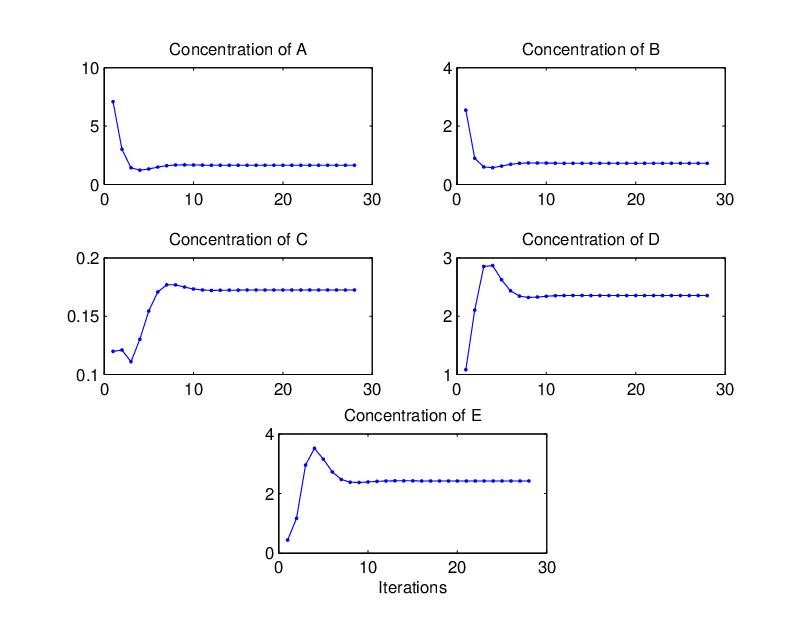
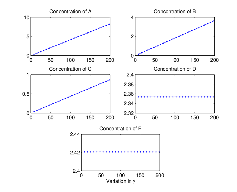
Figure 3 illustrates the change in steady state as a function of the total mass in the system, where total mass is defined as $\gamma=e^{T}(YDv^{\star}+YA^{T}\eta^{+}v^{\star}_{0})$ , as described in Theorem 1. The experiment shows that as the total mass increases, species $A$ , $B$ and $C$ adjust linearly to the additional mass, while species $D$ and $E$ stay at the same levels. This linear growth in species $A,B$ and $C$ can be explained analytically by the fact that the vector $\mathbf{1}$ lies in range of $Y^{T}$ .

3.3 Generating suitable networks

This section describes the sampling scheme used to generate random mass conserving chemical reaction networks with a prescribed number of terminal-linkage classes. The output of the method is a network with $n$ complexes, $m$ species, and $\ell$ strongly connected components, where $\ell$ is the desired number of terminal-linkage classes.

First, we iteratively generate Erdős-Réyni graphs¹¹ 1 An Erdős-Réyni graph is a directed unweighted graph. Each edge is included with probability $p$ and all edges are sampled iid. with $m$ nodes until we sample a graph with $\ell$ strongly connected components; call this graph $\hat{G}(\hat{V},\hat{E})$ . We give each edge in $\hat{E}$ a weight of an independent and uniformly distributed value in the range $(0,10]$ . These edge weights represent the reaction rates between complexes.

To generate the stoichiometry, we define a parameter $r$ as the maximum number of species in each complex. Each complex is constructed with a random sample of $q$ species, where $q$ is a random integer in $[1,r]$ . All samples are done uniformly and independently. Finally, we assign the multiplicity of each species in a complex with independent samples of the absolute value of a standard normal unit variance distribution. To ensure mass is conserved, we normalize the sum of the stoichiometry of the species that participate in a complex to one, so that $Y^{T}\mathbf{1}=\mathbf{1}$ and $A_{k}^{T}Y^{T}\mathbf{1}=\mathbf{0}$ .

3.4 Convergence of the Fixed Point Algorithm

This section illustrates the convergence of Algorithm 1 on large networks that consist of either a single terminal-linkage class or multiple terminal-linkage classes, i.e., weakly reversible networks.

Algorithm 1 produces sequences that, up to a small tolerance, satisfy (MA) at every iteration. Ideally, the infeasibility with respect to (FB) also monotonically decreases until convergence. Our extensive numerical experiments indicate that this is in fact the behavior for homogeneous networks that are weakly reversible.

Figure 4 displays the sequence of the infeasibilities $\|YA_{k}v_{k}\|_{\infty}$ at each iteration $k$ in Algorithm 1, for a network with a single terminal-linkage class, $50$ species and $500$ complexes, where at most $10$ species participate in each complex. Figure 5 displays the analogous sequence for a network of equal size and two terminal-linkage classes. We have observed this (apparently linear) convergence rate consistently over all generated networks, regardless of the number of terminal-linkage classes.

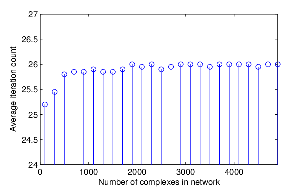
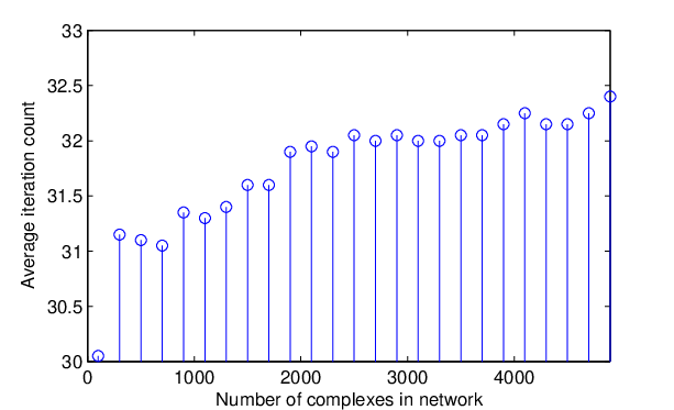
We have also investigated the number of iterations necessary for Algorithm 1 to converge on networks of different sizes, with either one or two terminal-linkage classes. Figures 6 and 7 display the mean number of iterations necessary for convergence on networks ranging from $100$ to $5000$ complexes, where each average is taken over $20$ instances per network size. Notably, the average number of iterations increases less than $10\%$ as the network size grows fifty-fold.

In future work, we plan to prove theoretical results on the existence of positive equilibria for chemical reaction networks with multiple terminal-linkage classes. However, our comprehensive numerical experiments seem to indicate that even for networks with more than one terminal-linkage class, there exists at least one positive fixed point of problem (3), and the iterates of Algorithm 1 converge to such a fixed point.

Finally, while conducting this work, we were made aware of related work by Deng et al. [2]. Their work extends that of Feinberg and Horn by proving that weak reversibility is a necessary and sufficient condition for existence of positive equilibria. While their proof is for closed systems (with $b=0$ ), it is not clear how to use the $0$ -complex in their extension to solve for any admissible $b$ , as mentioned in Section 1.1. More importantly, our proof is based on a less complicated convex optimization formulation, which gives a method to calculate numerical solutions using a fixed point algorithm.

Acknowledgment: We gratefully acknowledge Anne Shiu and her student for helpful discussions and directing us to [2].

References

[1] David F. Anderson. A proof of the global attractor conjecture in the single linkage class case. arXiv:1101.0761v3, 2011.
[2] Jian Deng, Martin Feinberg, Chris Jones, and Adrian Nachman. On the steady states of weakly reversible chemical reaction networks. (submitted), 2008.
[3] Martin Feinberg. Chemical reaction network structure and the stability of complex isothermal reactors I. The deficiency zero and deficiency one theorems. Chem. Eng. Sci., 42(10):2229–68, 1987.
[4] Martin Feinberg. Chemical reaction network structure and the stability of complex isothermal reactors II. Multiple steady states for networks of deficiency one. Chem. Eng. Sci., 43(1):1–25, 1988.
[5] R. M. T. Fleming, C. M. Maes, M. A. Saunders, Y. Ye, and B. Ø. Palsson. A variational principle for computing nonequilibrium fluxes and potentials in genome-scale biochemical networks. Journal of Theoretical Biology, 292:71–77, 2012.
[6] Jeremy Gunawardena. Chemical Reaction Network Theory for In-silico Biologists. Bauer Center For Genomics Research, Harvard University, Cambridge, MA, 2003.
[7] Fritz Horn. Necessary and sufficient conditions for complex balancing in chemical kinetics. Arch. Rational Mech. Anal., 49:172–186, 1972.
[8] Fritz Horn and Martin Feinberg. Dynamics of open chemical systems and the algebraic structure of the underlying reaction network. Chem. Eng. Sci., 29:775–787, 1974.
[9] Fritz Horn and Roy Jackson. General mass action kinetics. Archives of Rational Mech. Anal., 47:81–116, 1972.
[10] Jeffrey Orth, Ines Thiele, and Bernard Palsson. What is flux balance analysis? Nature Biotechnology, 28(3):245–248, 2010.
[11] Bernhard Palsson. Systems Biology: Properties of Reconstructed Networks. Cambridge University Press, 2006.
[12] John Ross. Thermodynamics and Fluctuations far from Equilibrium. Springer-Verlag, Berlin, Heidelberg, 2008.
[13] Michael Saunders. Primal-dual interior method for convex objectives. http://www.stanford.edu/group/SOL/software/pdco.html.