Gravity Dual Corrections to the Heavy Quark Potential at Finite-Temperature

Preprint: August 24, 2026

Hovhannes R. Grigoryan Yuri V. Kovchegov Affiliation: Department of Physics, The Ohio State University, Columbus, OH 43210, USA Affiliation: Email: grigoryan@physics.osu.edu Email: kovchegov.1@asc.ohio-state.edu Affiliation: E-mail addresses: ,

Abstract:

We apply gauge/gravity duality to compute $1/N^{2}_{c}$ corrections to the heavy quark potentials of a quark–anti-quark pair ( $Q\bar{Q}$ ) and of a quark–quark pair ( $QQ$ ) immersed into the strongly coupled ${\cal N}=4$ SYM plasma. On the gravity side these corrections come from the exchanges of supergravity modes between two string worldsheets stretching from the UV boundary of AdS space to the black hole horizon in the bulk and smeared over $S^{5}$ . We find that the contributions to the $Q\bar{Q}$ potential coming from the exchanges of all of the relevant modes (such as dilaton, massive scalar, 2-form field, and graviton) are all attractive, leading to an attractive net $Q\bar{Q}$ potential. We show that at large separations $r$ and/or high-temperature $T$ the potential is of Yukawa-type, dominated by the graviton exchange, in agreement with earlier findings. On the other hand, at small- $r\,T$ the $Q\bar{Q}$ potential scales as $\sim(1/r)\ln(1/r\,T)$ . In the case of $QQ$ potential the 2-form contribution changes sign and becomes repulsive: however, the net $QQ$ potential remains attractive. At large- $r\,T$ it is dominated by the graviton exchange, while at small- $r\,T$ the $QQ$ potential becomes Coulomb-like.

Keywords:

AdS/CFT, finite-temperature field theory, heavy quark potential

1 Introduction

Heavy quark potential in the vacuum of the ${\cal N}=4$ supersymmetric Yang-Mills (SYM) theory [1, 2] was one of the first results obtained using the Anti-de Sitter space/Conformal Field Theory (AdS/CFT) correspondence [3, 4, 5, 6, 7]. The first attempt to generalize the calculation [1, 2] to the case of the ${\cal N}=4$ SYM medium at finite temperature ( $T$ ) was made in [8, 9] shortly thereafter. The authors of [8, 9] identified two string configurations contributing to the finite-T heavy quark potential in the AdS/CFT framework, shown below in Fig. 2, and calculated their contributions. Defining the heavy quark potential as the free energy of the quark–anti-quark system immersed in the thermal bath, and assuming that the two string configuration from Fig. 2 contribute to the free energy on equal footing, the authors of [8, 9] obtained a potential which had a kink when plotted as a function of the quark–anti-quark separation $r$ . The kink (a derivative discontinuity) was due to a transition from the regime when one string configuration dominated the potential to the regime where another one was more important.

The kink feature of the result obtained in [8, 9] appears to be an artifact of the large- $N_{c}$ approximation, as was noted in [10, 11]. In [10, 11] it was argued that there are of the order of $N_{c}^{2}$ configurations with two straight strings (shown in the right panel of Fig. 2), such that the two configurations in Fig. 2 do not come in on equal footing, contrary to the assumption made in [8, 9]. Here $N_{c}$ is the number of D3 branes, and $N_{c}^{2}$ configurations may be interpreted as resulting from Chan-Paton indices of the two strings, each string having $N_{c}$ of indices (see also [12], where $N_{c}^{2}$ configurations emerge from the topological $Z_{N}\times Z_{N}$ symmetry of thermal SYM theory). This large number of string configurations enhances the terms which would be otherwise subleading. As was pointed out in [11], while the exchanges of supergravity fields between the straight strings shown in Fig. 3 are normally $N_{c}^{2}$ -suppressed, they become leading-order due to the fact that there are $N_{c}^{2}$ string configurations to enhance their contributions. The primary goal of [11] was determination of Debye mass, defined as the screening mass for chromo-electric modes in the plasma following [13]: therefore, for the heavy quark potential, the authors of [11] used the glueball masses calculated for QCD₃ from AdS/CFT correspondence in [14, 15], to obtain only the exponential form of the large- $r$ asymptotics of the contribution coming from the supergravity field exchanges to the heavy quark potential.

The question of the definition of the heavy quark potential at finite- $T$ in the context of AdS/CFT was raised in [16]. There it was pointed out that one can define two heavy quark potentials: color-singlet and color-adjoint [17, 18]. It was further conjectured in [16] that the hanging string configuration (left panel in Fig. 2) may correspond to the color-singlet potential, while the two-strings configuration (right panel in Fig. 2) may give the adjoint potential (which is zero in the large- $N_{c}$ limit). It was further suggested in [16] that the singlet potential at large- $r\,T$ , for which the solution corresponding to the hanging string configuration becomes complex, may be obtained by analytically continuing the solution into complex domain. Such analytic continuation led to an absorptive potential which had both real and imaginary parts, with the real part falling off as a power of $r$ at very large- $r$ , in some similarity to the weak-coupling perturbative results [19, 20, 21, 22, 23, 24, 25]. The issues associated with different definitions of the heavy quark potential are presented below in Sec. 2, where we present both definition of the finite- $T$ heavy quark potential, and discuss the pros and cons of using each of them.

The central goal of this paper is to find the full contribution to the heavy quark potential coming from the exchanges of supergravity fields between two straight strings oriented in opposite directions, as shown in Fig. 3 below. In the language of [16] this contribution would correspond to the color-adjoint potential. The calculation is presented in Sec. 3, and is carried out in Euclidean time, making it free of subtleties of the real-time formalism of thermal field theories. We concentrate on the case of the strings smeared over the $S^{5}$ , which correspond to Polyakov lines defined below in Eq. (17) averaged over the directions of their coupling to six scalars of ${\cal N}=4$ SYM. In this case the supergravity exchanges are limited to $k=0$ Kaluza-Klein (KK) modes. The contributions of all the relevant supergravity modes (dilaton, massive scalar, 2-form field and graviton) are calculated in detail in Sec. 3. We find that all the exchanges give attractive contributions to the $Q\bar{Q}$ potential. The net result for the $Q\bar{Q}$ potential in momentum space is shown in Fig. 13 (lower line). The potential turns out to be attractive at all values of $r\,T$ (which is the only relevant dimensionless parameter in the problem). The large- $r\,T$ asymptotics of the net $Q\bar{Q}$ potential is given by the exponential decay of Eq. (113), with the exponent determined by the first pole of the momentum ( $q$ )-space potential along the imaginary- $q$ axis (in agreement with [11]). The pole corresponds to the glueball mass in QCD₃ calculated in [14, 15]. We also find the residue of the pole (the factor in front of the exponential). The small- $r\,T$ asymptotics of the potential is rather peculiar, since it is not quite Coulomb-like, as can be seen from Eq. (114) below: the Coulomb $1/r$ term is multiplied by $\ln(1/r\,T)$ , generating a potential singularity in the $T\rightarrow 0$ limit. This singularity might be related to the instability of our non-BPS string configuration. We discuss how the quantum effects, such as string fluctuations, may come in to regulate this logarithmic divergence at very small- $r\,T$ .

Using the developed machinery, we also calculate the quark–quark $QQ$ potential in Sec. 4, for which there is no hanging (U-shaped) string configuration, and the only contribution comes from the exchanges shown in Fig. 14 between the two strings oriented in the same direction. The only difference between the $QQ$ potential and the adjoint contribution to the $Q\bar{Q}$ potential is in the sign of the NS 2-form contribution, which in the $QQ$ case becomes repulsive. The net $QQ$ potential is still attractive, and is plotted in momentum space in Fig. 13 (upper line). It is interesting to note that at short distances the $QQ$ potential becomes Coulomb-like, as shown in Eq. (136). The absence of the logarithmic singularity that we found earlier in the $Q\bar{Q}$ system can be related to the fact that the system of two parallel branes is (BPS) stable.

We summarize in Sec. 5 by suggesting that the 2-form exchange, which changes sign in going from $Q\bar{Q}$ to $QQ$ , may correspond to the chromo-electric modes in the gauge theory, while the exchanges of all other supergravity fields (the scalars and the graviton) may be interpreted as being mainly due to chromo-magnetic modes. Since both the $Q\bar{Q}$ and $QQ$ potentials are attractive we infer that at strong coupling magnetic modes are more important. We conclude by discussing the possibilities of improving on our calculation, including possibly making it more QCD-like.

2 Two definitions of the heavy quark potential at finite temperature

Here we will present possible interpretations of the observable we would like to calculate.

2.1 Singlet and octet potentials

Imagine immersing a very heavy quark and anti-quark into a static thermal medium of an $SU(N_{c})$ gauge theory. (For a nice pedagogical presentation of the topic, along with some weak-coupling calculations, we refer the reader to [18].) Working in the Euclidean time one defines the Polyakov loop operator at a spatial location $\vec{r}$ by

\displaystyle L({\vec{r}})\,=\,\text{P}\exp\left(i\,g\,\int\limits_{0}^{\beta}d\tau\,A_{0}({\vec{r}},\tau)\right)

(1)

with $\tau$ the Euclidean time, $A_{0}$ the temporal component of the gauge field, $\beta=1/T$ , and $T$ the temperature. Using Fierz identity one may write

\displaystyle\text{Tr}\,L^{\dagger}(0)\ \text{Tr}\,L({\vec{r}})\,=\,2\,\text{Tr}\left[t^{a}\,L^{\dagger}(0)\,t^{a}\,L({\vec{r}})\right]+\frac{1}{N_{c}}\,\text{Tr}\left[L^{\dagger}(0)\,L({\vec{r}})\right],

(2)

where $t^{a}$ are the generators of $SU(N_{c})$ in the fundamental representation, and $\vec{r}$ and $0$ are spatial locations of the quark and the anti-quark. One then defines the color-singlet heavy quark potential by

\displaystyle e^{-\beta\,V_{1}(r)}\,\equiv\,\frac{1}{N_{c}}\,\left\langle\text{Tr}\left[L^{\dagger}(0)\,L({\vec{r}})\right]\right\rangle_{c},

(3)

and the color-adjoint potential by

\displaystyle e^{-\beta\,V_{adj}(r)}\,\equiv\,\frac{2}{N_{c}^{2}-1}\,\left\langle\text{Tr}\left[t^{a}\,L^{\dagger}(0)\,t^{a}\,L({\vec{r}})\right]\right\rangle_{c}.

(4)

Here the angle brackets denote the expectation value of the operators in the thermal bath and the matrix elements are normalized to one for the case of no interaction. The distance between the quark and the anti-quark is $r=|{\vec{r}}|$ . The free energy of the quark–anti-quark pair in a thermal bath is given by

\displaystyle e^{-\beta\,F(r)}\,=\,\frac{1}{N_{c}^{2}}\,\left\langle\text{Tr}\,L^{\dagger}(0)\ \text{Tr}\,L({\vec{r}})\right\rangle_{c}.

(5)

The subscript $c$ in the above equations implies that we only keep the connected part of the correlator. This means that the contributions to the quark–anti-quark free energy and to the potentials due to self-interactions of the quarks are subtracted out. (The trivial disconnected part of the correlator due to the contribution without any (self-)interactions that gives $1$ in the perturbative expansion of the correlator is included on both sides of (5).)

Using the definitions (3), (4) and (5) in Eq. (2) we write [17, 18]

\displaystyle e^{-\beta\,F(r)}\,=\,\frac{1}{N_{c}^{2}}\,\left[e^{-\beta\,V_{1}(r)}+(N_{c}^{2}-1)\,e^{-\beta\,V_{adj}(r)}\right].

(6)

We see that the quark–anti-quark free energy consists of the singlet and adjoint contributions. One can show [18] that at weak coupling and in the large- $N_{c}$ limit the singlet potential $V_{1}(r)$ is of the order $g^{2}\,N_{c}$ with $g$ the gauge coupling, that is

\displaystyle V_{1}(r)\bigg|_{\lambda\ll 1,\,N_{c}\gg 1}\,\sim\,\lambda,

(7)

where $\lambda=g^{2}\,N_{c}$ is the ’t Hooft coupling. The singlet potential is also attractive at weak coupling [18], and maps onto the standard vacuum Coulomb potential at $T=0$ . The adjoint (octet) potential $V_{adj}(r)$ is repulsive at weak coupling [18], and is also subleading in the large- $N_{c}$ limit, such that

\displaystyle V_{adj}(r)\bigg|_{\lambda\ll 1,\,N_{c}\gg 1}\,\sim\,\frac{\lambda}{N_{c}^{2}}.

(8)

In the non-perturbative case, Eq. (3) is used in lattice QCD simulations to determine the singlet heavy quark potential at finite- $T$ (see e.g. [26]).

While the separation of the quark–anti-quark free energy into singlet and adjoint components appears to be possible in perturbative calculations order-by-order in the coupling [27, 28], it is less clear how to accomplish this decomposition in the general non-perturbative case. Indeed the definitions of $V_{1}(r)$ and $V_{adj}(r)$ in Eqs. (3) and (4) are not gauge-invariant. (The sum of the two contributions, and, therefore, the free energy, is gauge-invariant, as follows from Eq. (5).) We hence have a question of whether the singlet and adjoint potential are properly defined.

Refer to caption — Figure 1: Spatial Wilson loop described in the text.

One possible resolution of this problem is to define the color-singlet potential using the real (Minkowski) time formulation of thermal field theory. Define the temporal Wilson loop $W$ , which is a rectangle in the time– $\vec{r}$ plane, with the spatial sides connecting quark and anti-quark, and the temporal sides having length $\cal T$ , as depicted in Fig. 1. The singlet heavy quark potential can then be defined by¹¹ 1 Clearly this definition of the singlet potential is gauge-invariant, and is, in general, different from the definition in Eq. (3). However, the definition (9) of $V_{1}(r)$ does agree with that of Eq. (3) both in the lowest-order weak-coupling limit and in the strong-coupling AdS/CFT calculations.

\displaystyle V_{1}(r)\,=\,\lim_{{\cal T}\rightarrow\infty}\,\frac{i}{{\cal T}}\,\ln W.

(9)

After this definition of the singlet potential, and, after defining the quark–anti-quark free energy (in Euclidean time) with the help of Eq. (5), one may use Eq. (6) as the definition of the adjoint potential $V_{adj}(r)$ . Below, when calculating the adjoint potential, we will refer to the object defined by Eq. (6) with the help of Eqs. (9) and (5).

If one wants to calculate the Polyakov loop correlator (5) (with $L$ properly re-defined, as shown in Eq. (17) below) in the strongly-coupled ${\cal N}=4$ SYM theory using AdS/CFT correspondence, two distinct string configurations have to be considered, as shown in Fig. 2. The first AdS/CFT calculations of the finite- $T$ heavy quark potential, performed in [8, 9] following the zero-temperature calculation of [1, 2], found the contribution of the hanging string configuration from the left panel of Fig. 2. The leading-order contribution of the right panel in Fig. 2 is trivial, since, after subtracting the self-interactions of the quarks, which correspond to the actions of the two straight strings, we are left with zero answer for the renormalized action of this configuration, which is what one should expect in the non-interacting case. As we pointed out above there are of the order of $N_{c}^{2}$ configurations of straight strings. The setup appears to be similar to the decomposition of Eq. (6): just like in the gauge theory where one has one color-singlet configuration and $N_{c}^{2}-1$ color-adjoint configurations, there is one hanging string configuration and order- $N_{c}^{2}$ straight string configurations in Fig. 2. Moreover, the AdS/CFT result for the Polyakov loops correlator can be written as [16]

\displaystyle\frac{1}{N_{c}^{2}}\,\left\langle\text{Tr}\,L^{\dagger}(0)\ \text{Tr}\,L({\vec{r}})\right\rangle_{c}\propto\frac{e^{-S_{hanging}}+(N_{c}^{2}-1)\,e^{-S_{straight}}}{N_{c}^{2}}

(10)

with $S_{hanging}$ and $S_{straight}$ the actions of the hanging and straight string configurations, with the self-interactions removed by renormalization. (Indeed we only know that the coefficient in front of the second term on the right of Eq. (10) is of the order of $N_{c}^{2}$ and we do not have control over $-1$ , which we put there only to normalize the right-hand-side to one in the case of no interactions.) Comparing Eqs. (10) and (6) allowed the authors of [16] to suggest that the action of the hanging string configuration gives the singlet potential, while the action of the straight strings configuration gives the adjoint potential.

Since, as we have already noted, the decomposition of Eq. (6) is not gauge invariant, the suggestion of [16] still needs to be proven. However, let us use our real-time definition of the singlet potential from Eq. (9). For a Wilson loop from Fig. 1 with a very long temporal extent $\cal T$ , the AdS/CFT calculation, carried out in the Lorentzian-signature metric, would only contain the hanging string configuration. This is clear since the straight-strings configuration is impossible in Lorentzian-signature AdS₅: the orientation of the string should be the same throughout the single string world-sheet of this configuration, while orientations of the strings connecting to the quark and anti-quark are opposite, as shown in the right panel of Fig. 2, making this configuration impossible in real time. (In addition to that, in case of Lorentzian-signature black hole the straight-strings world-sheet would not be simply connected, indicating additional $1/N_{c}^{2}$ suppression.) Since the Nambu–Goto action of the static hanging string is independent of whether we work in Lorentzian or Euclidean signature metrics, the potential $V_{1}(r)$ defined by Eq. (9) is going to be the same as found in [8, 9]. Thus, using our definition of the singlet potential (9), we see that the hanging string configuration does indeed give a singlet potential identical to that in Eq. (3), yielding [8, 9]

\displaystyle V_{1}(r)\bigg|_{N_{c}\gg\lambda\gg 1}\,\sim\,\sqrt{\lambda}.

(11)

The fact that this potential is of the same order in $N_{c}$ as the weakly-coupled singlet potential in Eq. (7) indicates consistency of our conclusions with perturbative calculations.

Using Eq. (6), and remembering again that the hanging string configuration gives the singlet potential regardless of whether we work in real or imaginary time, we see that the straight strings configuration from Fig. 2 gives the adjoint potential. At the leading- $N_{c}^{2}$ order without any interactions between the strings the adjoint potential defined this way is zero. As was suggested in [11], a non-zero contribution to $S_{straight}$ comes from the interactions of the strings due to exchanges of supergravity fields, as shown in Fig. 3. Since the coupling of the supergravity fields to the string world-sheet is of the order of $1/N_{c}$ , the contribution to the two-strings action due to the exchanges shown in Fig. 3 is order- $1/N_{c}^{2}$ . Exchanges of supergravity fields between various string configurations have been considered before [29, 30, 31], yielding the interaction of the order of $\lambda/N_{c}^{2}$ . Identifying the diagram in Fig. 3 as the leading non-trivial contribution to the adjoint heavy quark potential, we conclude that at strong coupling

\displaystyle V_{adj}(r)\bigg|_{N_{c}\gg\lambda\gg 1}\,\sim\,\frac{\lambda}{N_{c}^{2}}.

(12)

Comparing this result to Eq. (8) we observe that, surprisingly, for the adjoint potential the power of ’t Hooft coupling $\lambda$ does not change in going from small to large $\lambda$ ! This is unlike the case of the singlet potential in which, just like in many other AdS/CFT results, the power of the coupling changes from $\lambda$ to $\sqrt{\lambda}$ as we increase it from very small to very large, as can be seen from Eqs. (7) and (11).

In the terminology of the two heavy quark potentials defined above, the goal of this paper is to calculate the contribution to the adjoint potential depicted in Fig. 2.

2.2 One unified potential

There exists an alternative to the singlet and adjoint potential decomposition.²² 2 We would like to thank Larry Yaffe for a discussion on this subject. One can simply define one unified heavy quark potential $V(r)$ as the free energy of the quark–anti-quark pair in the plasma, such that [32]

\displaystyle e^{-\beta\,V(r)}\,=\,\frac{1}{N_{c}^{2}}\,\left\langle\text{Tr}\,L^{\dagger}(0)\ \text{Tr}\,L({\vec{r}})\right\rangle_{c}.

(13)

The strength of this definition is that the heavy quark potential defined this way is manifestly gauge-invariant.

However, it appears difficult to find an intuitive physical interpretation for the single unified potential defined in Eq. (13). To see this, let us start with Eqs. (5) and (6), which, together with Eq. (13) give

\displaystyle e^{-\beta\,V(r)}\,=\,\frac{1}{N_{c}^{2}}\,\left[e^{-\beta\,V_{1}(r)}+(N_{c}^{2}-1)\,e^{-\beta\,V_{adj}(r)}\right].

(14)

Remembering from the previous Section that $V_{1}(r)\sim N_{c}^{0}$ and $V_{adj}(r)\sim 1/N_{c}^{2}$ (both at small and large coupling), we expand the right-hand-side of Eq. (14) in powers of $1/N_{c}^{2}$ to obtain [11]

\displaystyle e^{-\beta\,V(r)}\,=\,1+\frac{1}{N_{c}^{2}}\,\left[e^{-\beta\,V_{1}(r)}-1\right]-\beta\,V_{adj}(r)+O\left(\frac{1}{N_{c}^{4}}\right).

(15)

We see that the unified potential $V(r)$ has to be $N_{c}^{2}$ -suppressed and equal to

\displaystyle V(r)\,=\,\frac{1}{N_{c}^{2}}\,\frac{1}{\beta}\,\left[1-e^{-\beta\,V_{1}(r)}\right]+V_{adj}(r)+O\left(\frac{1}{N_{c}^{4}}\right).

(16)

It seems a bit counter-intuitive that the heavy quark potential at $T\neq 0$ should be $N_{c}^{2}$ -suppressed, while the $T=0$ potential is not. Also, in the $T\rightarrow 0$ limit, the singlet potential $V_{1}(r)$ maps smoothly onto the vacuum potential both at small [18] and large [1, 2] couplings: it is clear from Eq. (16) that the potential $V(r)$ instead goes to infinity in the $T\rightarrow 0$ limit. Moreover, at small quark–anti-quark separations $r$ , both in QCD and in ${\cal N}=4$ SYM theory, the singlet potential is $V_{1}(r)\sim-1/r$ (while $V_{adj}(r)\sim 1/r$ in QCD [18], and $V_{adj}(r)\sim-(1/r)\ln(1/r\,T)$ in ${\cal N}=4$ SYM at large- $\lambda$ , as we will show below). However, as one can infer from Eq. (16), the potential $V(r)$ diverges exponentially at small- $r$ as $-\exp(\text{const}\,\beta/r)$ , i.e., it becomes very strongly attractive: the physical origin of this behavior is not clear.

Despite the problems with its interpretation, the potential $V(r)$ is well-defined. As we have already mentioned, in our calculation below we will find the contribution of the exchanges of supergravity fields between the two straight strings pictured in Fig. 3. In the language of the unified potential $V(r)$ in Eq. (16), we will be constructing one of the contributions to this potential ( $V_{adj}(r)$ ) at order- $1/N_{c}^{2}$ , while the other contribution (coming from $V_{1}(r)$ ) was previously found in [8, 9].

3 The adjoint contribution to the $Q\bar{Q}$ potential

We want to find the contribution to the correlator of two Polyakov loops $\left\langle\text{Tr}\,L^{\dagger}(0)\ \text{Tr}\,L({\vec{r}})\right\rangle_{c}$ in ${\cal N}=4$ SYM theory at strong ’t Hooft coupling at order- $1/N_{c}^{2}$ . On the string theory or gravity side, these contribution will be coming from the interactions between the two straight strings in Fig. 3 . In ${\cal N}=4$ SYM theory the definition of the Polyakov loop operator suitable for AdS/CFT calculations is different from Eq. (1), and is given by [1, 29] (in Euclidean time)

\displaystyle L_{{\cal N}=4}({\vec{r}})\,=\,\text{P}\exp\left(i\,g\,\int\limits_{0}^{\beta}d\tau\,\left[A_{0}({\vec{r}},\tau)-i\,\theta^{I}({\vec{r}},\tau)\,X^{I}({\vec{r}},\tau)\right]\right),

(17)

where $X^{I}({\vec{r}},\tau)$ with $I=1,\ldots,6$ , are the six scalar fields of ${\cal N}=4$ SYM, and $\theta^{I}$ is a point on the unit five-sphere, which, for simplicity, will be taken to be independent of time. To make our results more QCD-like we will try to reduce their dependence on the scalar fields $X^{I}$ by averaging $L_{{\cal N}=4}$ over all $S^{5}$ angles $\theta^{I}$ .

At low energies type IIB string theory compactified on $AdS_{5}\times S^{5}$ contains a spectrum of supergravity modes. In the bosonic sector, the lightest modes are graviton $h_{MN}$ , dilaton $\phi$ , axion $C_{0}$ , Neveu–Schwarz (NS) $B_{MN}$ and Ramond–Ramond (RR) $C_{MN}$ 2-form fields ( $M,N=1,\ldots,5$ ), and RR 4-form field $C_{4}$ with a self-dual field strength. The spectrum also contains an infinite tower of massive scalars, $t^{k}$ ( $k\geq 0$ ) and $s^{k}$ ( $k\geq 2$ ) with $k$ the index of KK modes [33, 34, 35]. We are interested in those modes that couple to a string world-sheet (with the coupling that is least suppressed in $N_{c}$ ). The smearing of the string over the $S^{5}$ will effectively eliminate the coupling of the string world-sheet to modes that carry non-zero KK charge. In what follows, we will neglect the contribution of the fermionic sector to the interaction of the two string world-sheets, since it is $N_{c}^{2}$ -suppressed compared to that of the bosonic fields.

We want to find the quadratic fluctuations of those fields that couple to the string world-sheet as shown in Fig. 3 in the background of the AdS Schwarzschild black hole (AdSSBH) metric

\displaystyle ds^{2}

\displaystyle=\,g_{MN}\,dx^{M}\,dx^{N}\,=\,\frac{1}{z^{2}}\left[f(z)\,d\tau^{2}+dx^{i}dx^{i}+\frac{1}{f(z)}\,dz^{2}\right]\ ,\ \ \ \ f(z)=1-\frac{z^{4}}{z^{4}_{h}}\ ,

(18)

where $z\in(0,z_{h})$ is the direction along the extra fifth dimension, $x^{i}=(x^{1},x^{2},x^{3})$ are spacial coordinates, $\tau$ is the Euclidean time with period $\beta=\pi z_{h}$ , and $z_{h}$ determines the position of the black hole horizon, that is related to temperature as follows: $T=1/\beta=1/(\pi z_{h})$ .

To find the correlator of Polyakov loops at order- $1/N_{c}^{2}$ we will only need to consider exchanges of the fields that couple to string world-sheet at the tree level. Such fields are graviton, dilaton, massive scalars, and NS/RR two forms. The RR 2-form does not couple directly to a string world-sheet but it mixes with NS-NS 2-form, making it effectively massive [33, 15]. Notice that at the tree-level the axion only couples to the world-sheet fermions, which leads to a higher suppression in $N_{c}$ . Since we are interested in order- $1/N_{c}^{2}$ corrections, we will ignore the contribution to the correlator coming from the exchange of the axion.

As we argued above, the quantity we would like to calculate is

\displaystyle\frac{\left\langle\text{Tr}\,L^{\dagger}(0,{\vec{\theta}}^{\prime})\ \text{Tr}\,L({\vec{r}},{\vec{\theta}})\right\rangle}{\left\langle\text{Tr}\,L^{\dagger}(0,{\vec{\theta}}^{\prime})\right\rangle\,\left\langle\text{Tr}\,L({\vec{r}},{\vec{\theta}})\right\rangle}\Bigg|_{\text{adjoint}}\,=\,e^{-S_{straight}}\,=\,1-S_{straight}+O\left(\frac{1}{N_{c}^{4}}\right),

(19)

where we assume that the quark and anti-quark Polyakov line operators (17) are taken at fixed $S^{5}$ angles ${\vec{\theta}}$ and ${\vec{\theta}}^{\prime}$ correspondingly. Using the results of [29] we can write this contribution (somewhat schematically) in terms of the integrals over string world-sheets ${\cal A}$ and ${\cal A}^{\prime}$

\displaystyle\frac{\left\langle\text{Tr}\,L^{\dagger}(0,{\vec{\theta}}^{\prime})\ \text{Tr}\,L({\vec{r}},{\vec{\theta}})\right\rangle}{\left\langle\text{Tr}\,L^{\dagger}(0,{\vec{\theta}}^{\prime})\right\rangle\,\left\langle\text{Tr}\,L({\vec{r}},{\vec{\theta}})\right\rangle}\Bigg|_{\text{adjoint}}\,=\,\exp\left[\sum\limits_{k,m}Y_{m}^{(k)}(\theta)\,Y_{m}^{(k)}(\theta^{\prime})\,\int\frac{d{\cal A}}{2\,\pi\,\alpha^{\prime}}\,\frac{d{\cal A}^{\prime}}{2\,\pi\,\alpha^{\prime}}\,G_{k}(z,\tau;z^{\prime},\tau^{\prime})\right].

(20)

Here $G_{k}(z,\tau;z^{\prime},\tau^{\prime})$ is the sum of bulk-to-bulk propagators (multiplied by the appropriate vertex factors different for each field) for all the supergravity fields that couple to string world-sheets (parametrized by $z,\tau$ and $z^{\prime},\tau^{\prime}$ ), with the appropriate indices chosen for the graviton and 2-form contributions. The functions $Y_{m}^{(k)}(\theta)$ are spherical harmonics, $Y_{m}^{(k)}(\theta)\,=\,C_{I_{1}\ldots I_{k}}^{m}\,\theta_{I_{1}}\ldots\theta_{I_{k}}$ with $m$ labeling all harmonics corresponding to the state with the total angular momentum $J^{2}=k(k+4)$ and $C_{I_{1}\ldots I_{k}}^{m}$ a basis of symmetric traceless tensors such that $C_{I_{1}\ldots I_{k}}^{m_{1}}\,C^{I_{1}\ldots I_{k}\ m_{2}}=\delta^{m_{1}\,m_{2}}$ [36, 29]. As usual the slope parameter $\alpha^{\prime}=1/\sqrt{\lambda}$ .

Expanding Eq. (20) to the first non-trivial order, and averaging it along with Eq. (19) over $S^{5}$ angles $\theta$ and $\theta^{\prime}$ yields

\displaystyle\left\langle V_{adj}(r)\right\rangle_{\theta}\,=\,\frac{1}{\beta}\,\left\langle S_{straight}\right\rangle_{\theta}\,=\,\frac{1}{\beta}\,\int\frac{d{\cal A}}{2\,\pi\,\alpha^{\prime}}\,\frac{d{\cal A}^{\prime}}{2\,\pi\,\alpha^{\prime}}\,G_{0}(z,\tau;z^{\prime},\tau^{\prime})

(21)

since only $k=0$ KK mode survives the averaging and $Y_{0}^{0}=1$ in the conventions of [36, 29] that we have adopted. Below we will calculate $k=0$ KK mode contributions to the action $S_{straight}$ coming from the dilaton, massive scalar ( $t^{0}$ ), 2-form fields, and the graviton.

3.1 The Dilaton

3.1.1 Dilaton potential and the EOM

We begin with the simplest case of the dilaton exchange between the sting world-sheets pictured in Fig. 3. Writing the KK expansion for the dilaton field as $\phi=\sum_{k}\phi_{k}Y^{(k)}(\theta)$ , and only taking the lowest harmonic, the 10-dimensional dilaton action will be reduced to

\displaystyle S_{\phi}=\frac{N^{2}_{c}}{16\,\pi^{2}}\,\int d^{5}x\,\sqrt{g}~g^{MN}\,\partial_{M}\phi\,\partial_{N}\phi\ ,

(22)

where $\phi=\phi(x^{\mu},z)$ is the coefficient of the zeroth KK harmonic and $M,N=\mu,z$ with $\mu=0,\ldots,3$ . Notice, that the massless dilaton in the AdS bulk is dual to the glueball operator $\mathop{\rm Tr}F_{\mu\nu}^{2}$ in the boundary theory. The coupling of the dilaton to the string world-sheet is described by the action

\displaystyle S_{\phi-{\rm string}}=\frac{1}{2\pi\alpha^{\prime}}\int d^{2}\sigma~e^{\phi/2}\,\sqrt{\gamma}+\frac{1}{4\pi}\,\int d^{2}\sigma\,\sqrt{\gamma}\,R^{(2)}\,\phi\ ,

(23)

where $\gamma_{\alpha\beta}=g_{MN}\partial_{\alpha}x^{M}\partial_{\beta}x^{N}$ is the induced metric on the string world-sheet, and $R^{(2)}$ is the world-sheet curvature. In the large $N_{c}$ limit, when the AdS radius is large, $R^{(2)}$ will be subleading and can be ignored [29].

Expanding $e^{\phi/2}=1+\phi/2+\ldots$ and using $\alpha^{\prime}=1/\sqrt{\lambda}$ we see that the leading-order action of the dilaton coupled to two strings is

\displaystyle S_{{\rm dil}}\,=\,\frac{N^{2}_{c}}{16\,\pi^{2}}\,\int d^{5}x\,\sqrt{g}~g^{MN}\,\partial_{M}\phi\,\partial_{N}\phi+\frac{\sqrt{\lambda}}{4\pi}\,\int_{(1)}\,d^{2}\sigma\,\sqrt{\gamma}~\phi+\frac{\sqrt{\lambda}}{4\pi}\,\int_{(2)}\,d^{2}\sigma\,\sqrt{\gamma}~\phi\ ,

(24)

where $\int_{(i)}$ has a meaning of integration over the $i^{\rm th}$ string world-sheet, $i=1,2$ . The equations of motion (EOM) for the rescaled scalar field,

\displaystyle\bar{\phi}\,\equiv\,\frac{N^{2}_{c}}{2\,\pi\,\sqrt{\lambda}}\,\phi

(25)

can be written as

\displaystyle\frac{1}{\sqrt{g}}\,\partial_{M}\,\left[\sqrt{g}\,g^{MN}\,\partial_{N}\bar{\phi}_{i}\right]\,=\,\frac{\sqrt{\gamma}}{\sqrt{g}}\,\delta^{(3)}(\vec{x}-\vec{X}_{i})\ ,

(26)

where sub-index $i=1,2$ implies that we want to find the scalar field created by the string localized at spatial position $\vec{X}_{i}$ . Choosing the quark to be located at $\vec{X}_{1}=\vec{r}$ and the anti-quark at $\vec{X}_{2}=\vec{0}$ , the two strings world-sheets can be parametrized as

\displaystyle X_{1}^{M}=(\tau,{\vec{r}},z=\sigma),\ \ \ \ \ X_{2}^{M}=(\tau,{\vec{0}},z=z_{h}-\sigma)

(27)

with $\tau\in[0,\beta]$ and $\sigma\in[0,z_{h}]$ . Note that in Eq. (27) the string dual to the anti-quark ( $X_{2}$ ) is oriented opposite to that of the string dual to the quark ( $X_{1}$ ), as also shown in Fig. 3: this will be important for the analysis of the 2-form fields contribution.

Now, we are interested in evaluating the action (24) on the solution of the classical EOM (26). Taking into account that $\phi=\phi_{1}+\phi_{2}$ , and dropping the terms in the action that correspond to (anti-)quark self-energy contributions as they do not contribute to the connected Polyakov loop correlator in Eq. (19) that we want to find, we obtain

\displaystyle\overline{S}_{{\rm dil}}=\frac{\sqrt{\lambda}}{8\,\pi}\,\int_{(1)}d^{2}\sigma\sqrt{\gamma}~\phi_{2}+\frac{\sqrt{\lambda}}{8\,\pi}\,\int_{(2)}d^{2}\sigma\sqrt{\gamma}~\phi_{1}\ ,

(28)

where integration in each term is over one of the string world-sheets of the classical field $\phi$ created by the other string. Note that the two terms on the right-hand-side of Eq. (28) are equal. The integration over string world-sheet is

\displaystyle\int d^{2}\sigma\,=\,\int\limits_{0}^{\beta}d\tau\,\int\limits_{0}^{z_{h}}dz.

(29)

The determinant of the induced metric is $\gamma=\det\gamma_{\alpha\beta}=1/z^{4}$ for the strings parametrized as in Eq. (27) in the background metric (18). Using all this in Eq. (28), and noticing that in the static case considered here the solution of classical EOM (26) is going to be time-independent, we obtain the dilaton contribution to the potential

\displaystyle V_{adj}^{\phi}(r)\,=\,\frac{\lambda}{2\,N_{c}^{2}}\,\int\limits_{0}^{z_{h}}\frac{dz}{z^{2}}\,\bar{\phi}_{2}({\vec{r}},z).

(30)

As $\bar{\phi}_{2}$ is time-independent, we explicitly removed $\tau$ from its argument.

Since $g=\det g_{MN}=1/z^{10}$ the EOM (26) for $\bar{\phi}_{2}$ is

\displaystyle z^{3}\,\partial_{z}\left[\frac{f}{z^{3}}\,\partial_{z}\bar{\phi}_{2}\right]+{\vec{\nabla}}^{2}\,\bar{\phi}_{2}\,=\,z\,\delta^{(3)}(\vec{r}).

(31)

The equation is easier to tackle in momentum space. Writing

\displaystyle\bar{\phi}_{2}({\vec{r}},z)\,=\,\int\frac{d^{3}q}{(2\,\pi)^{3}}\,e^{i\,{\vec{q}}\cdot{\vec{r}}}\,\varphi({\vec{q}},z)

(32)

we recast Eq. (31) as

\displaystyle\left(1-\frac{z^{4}}{z^{4}_{h}}\right)\,\varphi_{zz}-\left(3+\frac{z^{4}}{z^{4}_{h}}\right)\,\frac{1}{z}\,\varphi_{z}-q^{2}\,\varphi=z

(33)

with $q^{2}={\vec{q}}^{\ 2}$ , $\varphi_{zz}=\partial_{z}^{2}\varphi$ , $\varphi_{z}=\partial_{z}\varphi$ . In solving Eq. (33) it is convenient to measure $z$ and $q$ in units of $z_{h}$ , such that, rescaling

\displaystyle\frac{z}{z_{h}}\,\rightarrow\,z,\ \ \ q\,z_{h}\,\rightarrow\,q,\ \ \ \frac{\varphi}{z_{h}^{3}}\,\rightarrow\,\varphi

(34)

to make them dimensionless, we get

\displaystyle\left(1-z^{4}\right)\,\varphi_{zz}-\left(3+z^{4}\right)\,\frac{1}{z}\,\varphi_{z}-q^{2}\,\varphi\,=\,z.

(35)

The potential in momentum space $V_{adj}(q)$ is defined by

\displaystyle V_{adj}(r)\,=\,\frac{1}{z_{h}}\,\int\frac{d^{3}q}{(2\,\pi)^{3}}\,e^{i\,{\vec{q}}\cdot{\vec{r}}}\,V_{adj}(q),

(36)

where we have switched to dimensionless ${\vec{r}}/z_{h}\,\rightarrow\,{\vec{r}}$ as well. The dimensionless momentum-space dilaton contribution to the potential is

\displaystyle V_{adj}^{\phi}(q)\,=\,\frac{\lambda}{2\,N_{c}^{2}}\,\int\limits_{0}^{1}\frac{dz}{z^{2}}\,\varphi(q,z).

(37)

(Note that the rescaled $\varphi$ in Eq. (37) is dimensionless, and so are the rescaled $z$ and $q$ .) Since Eq. (35) depends on $\vec{q}$ through $q^{2}$ , its solution $\varphi$ depends on the vector $\vec{q}$ through its length squared $q^{2}$ .

3.1.2 Solution of the dilaton EOM

Solution of the dilaton EOM (35) can be constructed as a series in the powers of $z$

\displaystyle\varphi\,=\,\sum_{n=0}^{\infty}\,\frac{b_{n}\,z^{2\,n+3}}{2\,n+3}+C^{\phi}(q^{2})\,\sum_{n=0}^{\infty}\,\frac{f_{n}\,z^{2\,n+4}}{2\,n+4}

(38)

with the recursion relations for the coefficients


	$\displaystyle b_{n}\,=\,\frac{q^{2}}{(2\,n-1)\,(2\,n+1)}\,b_{n-1}+b_{n-2},\ \ \ \ \ b_{0}=-1,\ \ b_{1}=-\frac{q^{2}}{3},$		(39a)

	$\displaystyle f_{n}\,=\,\frac{q^{2}}{2\,n\,(2\,n+2)}\,f_{n-1}+f_{n-2},\ \ \ \ \ f_{0}=1,\ \ f_{1}=\frac{q^{2}}{8}.$		(39b)

The first series in Eq. (38) is the solution of the inhomogeneous equation, while the second series is the solution of the homogeneous equation. Both series were constructed by requiring that $\varphi(z=0)=0$ : this is the condition of normalizability of the dilaton field. Clearly the potential in (37) would be infinite if this condition was not satisfied. The coefficient $C^{\phi}(q^{2})$ in Eq. (38) has to be fixed by the boundary condition at the horizon. To obtain this condition we follow the standard procedure and expand the AdSSBH metric (18) near horizon. Defining $\rho=2\sqrt{1-z}$ we obtain a flat near-horizon metric

\displaystyle ds^{2}\big|_{\rho\approx 0}\,\approx\,\rho^{2}d\tau^{2}+d\rho^{2}+d{\vec{x}}^{\ 2}.

(40)

In this new flat metric the function $\varphi(x,\rho)$ should have zero derivative at the origin, $\varphi_{\rho}(\rho=0)=0$ , otherwise $\varphi$ would have a discontinuous derivative at the origin.³³ 3 We thank Samir Mathur for pointing out this argument to us. This translates into

\displaystyle\left\{\sqrt{1-z}\,\varphi_{z}\right\}\big|_{z=1}\,=\,0

(41)

in $z$ -space. The condition (41) appears to be somewhat weak, as it only implies that $\varphi$ should be finite at the horizon. To see that the finiteness of $\varphi$ at the horizon uniquely determines the solution of Eq. (35) we can expand $\varphi$ in the powers of $1-z$ . In this near-horizon expansion case the series solving the inhomogeneous and homogeneous equations (35) are the same, such that the solution can be written as a single series

\displaystyle\varphi\,=\,\sum_{n=0}^{\infty}\,h_{n}\,(1-z)^{n}

(42)

with the recursion relations

	$\displaystyle h_{n}\,=\,$	$\displaystyle\frac{2\,(n-1)\,(5\,n-8)+q^{2}}{4\,n^{2}}\,h_{n-1}-\frac{2\,(n-2)\,(5\,n-12)+q^{2}}{4\,n^{2}}\,h_{n-2}$
		$\displaystyle+\frac{(n-3)\,(5\,n-16)}{4\,n^{2}}\,h_{n-3}-\frac{(n-4)^{2}}{4\,n^{2}}\,h_{n-4}+\frac{1}{4}\,\delta_{n1}-\frac{1}{8}\,\delta_{n2}+\frac{1}{36}\,\delta_{n3}$		(43)

between its coefficients. One can see that the value of $\varphi$ at the horizon $z=1$ , given by the coefficient $h_{0}$ , is assumed to be finite here. The coefficient $h_{0}$ alone determines the rest of the series (42), with the help of Eq. (43). The only remaining degree of freedom, $h_{0}$ , is fixed by the $\varphi(z=0)=0$ condition. This proves that finiteness of $\varphi$ at the horizon, along with the $\varphi(z=0)=0$ condition, are sufficient to uniquely define the solution of Eq. (35).

Analytic summation of the series (38) and/or (42) appears to be prohibitively complicated. Instead we construct the solution for $\varphi$ by summing the series (38) numerically. We numerically evaluate partial sums

\displaystyle\varphi(q,z,N)\,=\,\sum_{n=0}^{N}\,\frac{b_{n}\,z^{2\,n+3}}{2\,n+3}+C^{\phi}(q^{2},N)\,\sum_{n=0}^{N}\,\frac{f_{n}\,z^{2\,n+4}}{2\,n+4}

(44)

constructing sequential approximations $\varphi(q,z,N)$ of the exact solution $\varphi(q,z)=\lim\limits_{N\rightarrow\infty}\varphi(q,z,N)$ . To determine the coefficients $C^{\phi}(q^{2},N)$ we need to require that $\varphi(q,z,N)$ is finite at the horizon: to insure this without specifying the (unknown) value of $\varphi(q,z,N)$ at the horizon we impose Neumann boundary conditions on $\varphi(q,z,N)$ at $z=1$ . Indeed the exact solution of Eq. (35) does not have to satisfy Neumann boundary conditions at the horizon: however, imposing this condition on partial sums $\varphi(q,z,N)$ makes them finite at the horizon, such that, since the solution which is finite at the horizon is unique, as $N$ increases the partial sums would converge onto this one exact solution for $\varphi(q,z)$ , with the part of the interval $z\in(0,1)$ affected by the Neumann boundary condition rapidly shrinking. Since Eq. (35) is a second-order differential equation, it has two solutions: one that is finite at the horizon, and one that is infinite at the horizon. Therefore any boundary condition forcing $\varphi(q,z,N)$ to be finite at $z=1$ would map these partial sums onto the solution finite at the horizon in the $N\rightarrow\infty$ limit. For instance, Dirichlet boundary condition at $z=1$ would also work. However, Neumann boundary conditions appear to give the fastest numerical convergence to the exact solution.

Demanding that $\partial_{z}\varphi(q,z,N)\big|_{z=1}=0$ yields

\displaystyle C^{\phi}(q^{2},N)\,=\,-\frac{\sum_{n=0}^{N}\,b_{n}}{\sum_{n=0}^{N}\,f_{n}}.

(45)

Using Eq. (45) in Eq. (44) we construct a series of numerical approximations to the solution of Eq. (35). Three approximate solutions are plotted in Fig. 4 for different values of $N$ . One can see that, as the order of the partial sum $N$ increases, the solutions tend to converge to the unified limiting curve, deviating from it only in the rapidly shrinking region near $z=1$ to satisfy Neumann boundary condition.

Since we are interested in the dilaton contribution to the heavy quark potential $V_{adj}^{\phi}(q)$ we use Eq. (38) in Eq. (37) to obtain

\displaystyle V_{adj}^{\phi}(q)\,=\,\frac{\lambda}{2\,N_{c}^{2}}\,\left[\sum_{n=0}^{\infty}\,\frac{b_{n}}{(2\,n+2)\,(2\,n+3)}+C^{\phi}(q^{2})\,\sum_{n=0}^{\infty}\,\frac{f_{n}}{(2\,n+3)\,(2\,n+4)}\right].

(46)

The potential is also evaluated by numerical calculation of the partial sums. Dilaton contribution $V_{adj}^{\phi}(q)$ to the heavy quark potential is plotted in momentum space in Fig. 5. The potential is finite at $q=0$ which indicates screening of the quark–anti-quark interactions by the thermal ${\cal N}=4$ SYM medium. Since the potential is monotonically increasing and negative, one should expect that in coordinate space the contribution of the dilaton will be attractive.

3.1.3 Asymptotics of the dilaton contribution

While it is hard to perform a reliable numerical Fourier transform of the potential from Fig. 5 into coordinate space, we can use our numerical results to understand its asymptotics at large and small values of the dimensionless parameter $r$ , or, equivalently, of the parameter $r\,T$ if we go back to the dimensionful $r$ not measured in the units of $z_{h}$ .

Let us begin with the case of large- $r\,T$ , which can be achieved by either increasing the quark–anti-quark separation $r$ or by increasing the temperature $T$ . Noting that the momentum space potential is a function of $q^{2}$ we can integrate Eq. (36) over the angles, obtaining

\displaystyle V_{adj}(r)\,=\,\frac{-i}{(2\,\pi)^{2}}\,\frac{1}{r\,z_{h}}\,\int\limits_{-\infty}^{\infty}dq\ q\,e^{i\,q\,r}\,{\tilde{V}}_{adj}(q^{2}).

(47)

The $q$ -integral can be done by closing the contour in the upper half-plane and picking up contributions of all the singularities there. It turns out that the singularities of the dilaton potential $V_{adj}^{\phi}(q)$ (along with the similar potentials for other supergravity fields that we will analyze below) are only limited to poles along the imaginary- $q$ axis. As originally suggested in [11], the positions of the poles correspond to the glueball masses for QCD₃ calculated in [14, 37, 15, 38, 39, 40] and references therein. The potential $V_{adj}^{\phi}(q)$ is plotted in units of $\lambda/(2\,N_{c}^{2})$ along the positive imaginary- $q$ axis in Fig. 6, illustrating this point. Note that the potential is real along both the real and the imaginary axes in the complex $q$ -plane.

Denoting the positions of the poles on the positive imaginary- $q$ axis by $i\,m_{n}$ with $n=1,2,\ldots$ (such that $m_{1}<m_{2}<\ldots$ ) we write (see also [30, 37])⁴⁴ 4 In Eq. (48) we assume that the poles are order one: we have explicitly verified this only for the first pole for each supergravity particle analyzed.

\displaystyle V_{adj}(r)\,=\,\frac{1}{2\,\pi\,r\,z_{h}}\,\sum_{n=1}^{\infty}i\,m_{n}\,e^{-m_{n}\,r}\,\lim_{q\,\rightarrow\,i\,m_{n}}\left[(q-i\,m_{n})\,V_{adj}(q^{2})\right].

(48)

The large- $r$ behavior is determined by the first pole $m_{1}$ .

For the case of the dilaton, according to our numerical solution the leading pole is at $m_{1}^{\phi}=3.4041\pm 0.0001$ (for $N=3\times 10^{5}$ iterations), in agreement with [14, 15]. The residue of the pole is $i\,(0.12\pm 0.01)$ , such that the large- $r$ asymptotics of the dilaton contribution to the potential is

\displaystyle V_{adj}^{\phi}(r)\bigg|_{r\,T\gg 1}\,\approx\,-\frac{\lambda}{2\,N_{c}^{2}}\,\frac{0.41\pm 0.04}{2\,\pi\,r}\,e^{-3.4041\,\pi\,r\,T},

(49)

where we have inserted $z_{h}=1/(\pi\,T)$ back into the expression. We obtain a screened Yukawa-type attractive potential falling off exponentially with the distance $r$ .

Now we consider the case of small- $r$ , which, inserting $z_{h}$ back, means small $r\,T$ , a regime which can be interpreted as resulting from either the short separations $r$ or low temperatures $T$ . Due to the Fourier transform (36), low- $r$ corresponds to large- $q$ . In the large- $q$ limit, and for $z\gg 1/q$ , we can neglect the terms on the left-hand-side of Eq. (35) containing $z$ -derivatives compared to the term with $q^{2}$ . This yields

\displaystyle\varphi\big|_{q\,z\gg 1}\,\approx\,-\frac{z}{q^{2}}.

(50)

Since, as follows from the series solution (38), the function $\varphi$ goes to zero as $z^{3}$ when $z\rightarrow 0$ , we can argue that most of the support of the integrand $\varphi/z^{2}$ in Eq. (37) comes from larger $z$ , and hence, for large- $q$ , the condition $q\,z\gg 1$ is satisfied over most of the $z$ -range contributing to the potential. Using Eq. (50) in Eq. (37) and inserting a UV cutoff of $1/q$ in it, we obtain (with the leading logarithmic accuracy)

\displaystyle V_{adj}^{\phi}(q)\bigg|_{q\gg 1}\,\approx\,-\frac{\lambda}{2\,N_{c}^{2}}\,\frac{1}{q^{2}}\,\ln q.

(51)

Fourier-transforming this back into coordinate space with the help of Eq. (36), and inserting $z_{h}$ back in to make $r$ dimensionful yields (again with the leading logarithmic accuracy)

\displaystyle V_{adj}^{\phi}(r)\bigg|_{r\,T\ll 1}\,\approx\,-\frac{\lambda}{2\,N_{c}^{2}}\,\frac{1}{4\,\pi\,r}\,\ln\frac{1}{r\,T}.

(52)

The potential in (52) is attractive, but is not quite Coulomb-like, due to the extra logarithmic factor. This factor is somewhat worrisome, as it makes the potential infinite in the $T\rightarrow 0$ limit. This, however, might not be viewed as a problem on the gauge theory side, since it is not clear how to define the adjoint potential at $T=0$ in a gauge-invariant way: therefore, the divergence takes place in the limit when the quantity we are calculating is not defined. On the string theory side it appears that, in absence of the black hole, the interaction between two string world-sheets would be infinite: the situation is analogous to the instability of the parallel D-brane–anti-D-brane configuration. One may also argue that at small separations $r$ higher-order string corrections may come in and modify the result, possibly regulating the divergence: we will discuss this possibility after calculating the contributions of all other supergravity fields.

3.2 Massive Scalars

3.2.1 The potential and EOM

In addition to the dilaton, compactification on $S^{5}$ leads to additional scalar modes that come from the KK modes of the trace of the metric and from the 4-form field perturbations over $S^{5}$ , that is, from $h^{\alpha}_{\alpha}$ and $a_{\alpha\beta\gamma\delta}$ correspondingly, where indices take values on $S^{5}$ [33, 36, 29, 34, 35]. The KK modes of $h^{\alpha}_{\alpha}$ and $a_{\alpha\beta\gamma\delta}$ mix in the EOM, but at the quadratic order the action can be diagonalized by the scalar modes $s^{k}$ (with $k\geq 2$ ) and $t^{k}$ (with $k\geq 0$ ) [33, 36, 29, 34, 35]. The modes $s^{k}$ for $k=2,3$ are tachyonic, while all other $s^{k}$ and all $t^{k}$ modes are massive: we will refer to all modes $t^{k}$ and $s^{k}$ as massive scalars. Since we are interested in the modes which survive averaging over $S^{5}$ , i.e., in $k=0$ KK modes, we only need to study the contribution of $t^{0}$ to the string interaction. The action for the $t^{k}$ modes can be found in [34, 35]. The coupling of $t^{k}$ to the string world-sheet follows from the coupling of the graviton to the string. Writing the 5d metric fluctuations for $k=0$ KK mode in terms of fields diagonalizing EOM as [35]

\displaystyle\delta g_{MN}^{0}\,=\,h_{MN}^{0}-\frac{40}{3}\,g_{MN}\,t^{0}+\frac{4}{3}\,\nabla_{M}\,\nabla_{N}\,t^{0}

(53)

with $\nabla_{M}$ the covariant derivative we can determine the coupling of $t^{0}$ to the string world-sheet from the coupling of $\delta g_{MN}^{0}$ to the string. One can readily show that the coupling of the $\nabla_{M}\,\nabla_{N}\,t^{0}$ term to the world-sheet of our straight strings (27) is zero if $\partial_{z}t^{0}(z=0)=0$ , with the latter condition satisfied by the solution of the classical EOM for $t^{0}$ . Dropping the derivative term in Eq. (53) we get (using the same notation as in Eq. (24))

\displaystyle S_{t^{0}}\,=\,\frac{80}{3}\,\frac{N^{2}_{c}}{\pi^{2}}\,\int d^{5}x\,\sqrt{g}\,\left[g^{MN}\,\partial_{M}t^{0}\,\partial_{N}t^{0}+32(t^{0})^{2}\right]+\frac{20}{3}\,\frac{\sqrt{\lambda}}{\pi}\,\int\limits_{(1)}\,\frac{d\tau\,dz}{z^{2}}\ t^{0}+\frac{20}{3}\,\frac{\sqrt{\lambda}}{\pi}\,\int\limits_{(2)}\,\frac{d\tau\,dz}{z^{2}}\,t^{0}.

(54)

Rescaling the $t^{0}$ field

\displaystyle\bar{t}^{\ 0}\,\equiv\,\frac{8\,N^{2}_{c}}{\pi\,\sqrt{\lambda}}\,t^{0}

(55)

we write the equation of motion for the field produced by the string at ${\vec{X}}_{2}={\vec{0}}$ :

\displaystyle\frac{1}{\sqrt{g}}\,\partial_{M}\,\left[\sqrt{g}\,g^{MN}\,\partial_{N}\bar{t}^{\ 0}\right]-32\,\bar{t}^{\ 0}\,=\,z^{3}\,\delta^{(3)}(\vec{x})\ .

(56)

The action evaluated at the classical solution is

\displaystyle{\overline{S}}_{t^{0}}\,=\,\frac{5}{6}\,\frac{\lambda}{N_{c}^{2}}\,\int\limits_{0}^{\beta}d\tau\,\int\limits_{0}^{z_{h}}\frac{dz}{z^{2}}\ \bar{t}^{\ 0}({\vec{r}},z)

(57)

giving the contribution to the heavy quark potential

\displaystyle V^{t^{0}}_{adj}(r)\,=\,\frac{5}{6}\,\frac{\lambda}{N_{c}^{2}}\,\int\limits_{0}^{z_{h}}\frac{dz}{z^{2}}\,\bar{t}^{\ 0}({\vec{r}},z).

(58)

Just like with the dilaton, in order to solve Eq. (56) we go to momentum space

\displaystyle\bar{t}^{0}({\vec{r}},z)\,=\,\int\frac{d^{3}q}{(2\,\pi)^{3}}\,e^{i\,{\vec{q}}\cdot{\vec{r}}}\,{\gothfamily t}^{0}({\vec{q}},z),

(59)

where, in units of $z_{h}$ (34), the EOM becomes

\displaystyle\left(1-z^{4}\right)\,{\gothfamily t}^{0}_{zz}-\left(3+z^{4}\right)\,\frac{1}{z}\ {\gothfamily t}^{0}_{z}-q^{2}\,{\gothfamily t}^{0}\,-\frac{32}{z^{2}}\,{\gothfamily t}^{0}\,=\,z.

(60)

Just like with the dilaton we require that ${\gothfamily t}^{0}(z=0)=0$ and ${\gothfamily t}^{0}(z=1)$ is finite. The contribution of $t^{0}$ to the momentum-space potential is then (in the same $z_{h}=1$ units)

\displaystyle V_{adj}^{t^{0}}(q)\,=\,\frac{5}{6}\,\frac{\lambda}{N_{c}^{2}}\,\int\limits_{0}^{1}\frac{dz}{z^{2}}\ {\gothfamily t}^{0}(q,z).

(61)

The coordinate-space potential can be obtained from Eq. (36).

3.2.2 Solution of the EOM for $t^{0}$

The series solution for Eq. (60) is

\displaystyle{\gothfamily t}^{0}\,=\,\sum_{n=0}^{\infty}\,c_{n}\,z^{2\,n+3}+C^{t^{0}}(q^{2})\,\sum_{n=0}^{\infty}\,g_{n}\,z^{2\,n+8}

(62)

with the recursion relations for the coefficients


	$\displaystyle c_{n}\,=\,\frac{q^{2}}{(2\,n-5)\,(2\,n+7)}\,c_{n-1}+\frac{(2\,n-1)^{2}}{(2\,n-5)\,(2\,n+7)}\,c_{n-2},\ \ \ \ \ c_{0}=-\frac{1}{35},\ \ c_{1}=\frac{q^{2}}{945},$		(63a)

	$\displaystyle g_{n}\,=\,\frac{q^{2}}{4\,n\,(n+6)}\,g_{n-1}+\frac{(n+2)^{2}}{n\,(n+6)}\,g_{n-2},\ \ \ \ \ g_{0}=1,\ \ g_{1}=\frac{q^{2}}{28}.$		(63b)

Again we sum the series (62) numerically, imposing the Neumann boundary conditions at the horizon. These yield

\displaystyle C^{t^{0}}(q^{2},N)\,=\,-\frac{\sum_{n=0}^{N}\,c_{n}\,(2\,n+3)}{\sum_{n=0}^{N}\,g_{n}\,2\,(n+4)}.

(64)

Substituting Eq. (62) into Eq. (61) we obtain the contribution of the scalar $t^{0}$ to the momentum-space heavy quark potential

\displaystyle V_{adj}^{t^{0}}(q)\,=\,\frac{5}{6}\,\frac{\lambda}{N_{c}^{2}}\,\left[\sum_{n=0}^{\infty}\,\frac{c_{n}}{2\,(n+1)}+C^{t^{0}}(q^{2})\,\sum_{n=0}^{\infty}\,\frac{g_{n}}{2\,n+7}\right].

(65)

The potential $V_{adj}^{t^{0}}(q)$ is plotted in Fig. 7 in units of $\lambda/(2N_{c}^{2})$ . It looks similar to the dilaton contribution to the potential plotted in Fig. 5 and also appears to be attractive.

3.2.3 Asymptotics of the massive scalar contribution

Just like for the dilaton, the singularities of the potential ${\tilde{V}}_{adj}^{t^{0}}(q)$ are poles along the imaginary- $q$ axis. The potential $V_{adj}^{t^{0}}(q)$ along the positive imaginary- $q$ axis is plotted in Fig. 8.

The large- $r$ asymptotics is given by the leading pole, which was found to be at $m_{1}^{t^{0}}=7.410\pm 0.001$ (for $N=10^{6}$ iterations), in minor disagreement with [15], possibly due to differences in implementation of the numerical simulations. The residue of the pole is $i\,(0.04\pm 0.01)$ , giving the large- $r$ asymptotics of the $t^{0}$ contribution to the heavy quark potential

\displaystyle V_{adj}^{t^{0}}(r)\bigg|_{r\,T\gg 1}\,\approx\,-\frac{5}{6}\,\frac{\lambda}{N_{c}^{2}}\,\frac{0.30\pm 0.08}{2\,\pi\,r}\,\,e^{-7.410\,\pi\,r\,T}

(66)

with $z_{h}=1/(\pi\,T)$ inserted back such that $r$ has units of distance. Again, this is an attractive screened Yukawa-type potential, with the screening mass larger than that for the dilaton. Hence the dilaton contribution dominates over that of $t^{0}$ at large- $r\,T$ .

We have also investigated the contribution of the tachyonic scalar $s^{2}\equiv s^{k=2}$ to the interaction between the string world-sheets. Since this is a $k=2$ KK mode, it does not contribute to the potential (21) averaged over $S^{5}$ positions of both strings that we want to calculate. In the effort to translate the physical meaning of the $s^{2}$ contribution into the QCD language, and identifying the $SU(4)$ $R$ -symmetry group of ${\cal N}=4$ SYM with the flavor group on QCD, one may argue that $s^{2}$ -exchange would correspond to some flavor-changing interaction between the quarks. Our motivation for studying $s^{2}$ lies in the fact it is a tachyon, and it is precisely the $s^{2}$ contribution which dominates the large- $r$ asymptotics of the interactions of two strings in the empty AdS₅ space (zero-temperature case in the gauge theory), as was shown in [29], giving a potential between two rectangular Wilson loops (two “mesons”) that falls of as $1/r^{4}$ at large- $r$ . The $s^{2}$ -exchange in the AdSSBH background leads to an attractive potential, but with a small screening mass $m_{1}^{s^{2}}\approx 1.373\pm 0.001$ (for $N=10^{5}$ iterations), such that

\displaystyle V_{adj}^{s^{2}}(r)\bigg|_{r\,T\gg 1}\,\propto\,-\frac{\lambda}{N_{c}^{2}}\,\frac{1}{r}\,\,e^{-1.373\,\pi\,r\,T}.

(67)

Clearly, if we allow for exchanges of higher KK modes, the $s^{2}$ contribution would dominate over that of the dilaton and $t^{0}$ at large- $r\,T$ . We would like to point out in advance that the screening masses for the 2-form field and the graviton ( $k=0$ term only) would also be larger than $m_{1}^{s^{2}}\approx 1.373$ . As the screening mass appears to increase with $k$ , one may conjecture that the $s^{2}$ contribution (67) would dominate over all other supergravity modes exchanges at large- $r\,T$ . Since our main analysis here is limited to $k=0$ case when quarks do not carry $R$ -charge, we will not have the $s^{2}$ contribution in the net potential.

At small- $r$ /large- $q$ the approximate solution of Eq. (60) is

\displaystyle{\gothfamily t}^{0}\big|_{q\,z\gg 1}\,\approx\,-\frac{z}{q^{2}},

(68)

giving the coordinate-space potential

\displaystyle V_{adj}^{t^{0}}(r)\bigg|_{r\,T\ll 1}\,\approx\,-\frac{5}{6}\,\frac{\lambda}{N_{c}^{2}}\,\frac{1}{4\,\pi\,r}\,\ln\frac{1}{r\,T},

(69)

where again we have reinstated the temperature $T$ explicitly.

3.3 Two-Form Fields

3.3.1 The potential and EOM

The effective action for the $k=0$ KK mode of the NS 2-form along with its coupling to the string world-sheet can be written as (after integrating out the contribution of the RR 2-form)

	$\displaystyle S_{B}=$	$\displaystyle\frac{1}{24\,\kappa^{2}_{5}}\,\int d^{5}x\sqrt{g}~H_{MNR}\,H^{MNR}+\frac{2}{\kappa^{2}_{5}}\,\int d^{5}x\sqrt{g}~B_{MN}B^{MN}$
		$\displaystyle+\frac{\xi}{4\pi\alpha^{\prime}}\,\epsilon^{ab}\,\int\limits_{(1)}d^{2}\sigma~B_{MN}\,\partial_{a}X^{M}\,\partial_{b}X^{N}+\frac{\xi}{4\pi\alpha^{\prime}}\,\epsilon^{ab}\,\int\limits_{(2)}d^{2}\sigma~B_{MN}\,\partial_{a}X^{M}\,\partial_{b}X^{N}\ ,$		(70)

where indices $a,b=0,1$ run over string world-sheets, $\epsilon^{ab}=-\epsilon^{ba}$ with $\epsilon^{01}=1$ , and $\kappa_{5}^{2}=4\pi^{2}/N^{2}_{c}$ . As usual

\displaystyle H_{MNR}\,=\,\partial_{M}\,B_{NR}+\partial_{N}\,B_{RM}+\partial_{R}\,B_{MN}.

(71)

The coefficient $\xi$ is equal to $1$ when both indices $M,N$ of $B_{MN}$ in the same term are spatial, i.e., when $M,N=\mu,\nu=1,\ldots,4$ , and $\xi=i$ when either $M$ or $N$ is $0$ . This extra factor of $i$ arises due to the transition to Euclidean-signature space with $B_{0\mu}^{\text{Minkowskian}}=i\,B_{0\mu}^{\text{Euclidean}}$ , where $\mu=1,\ldots,4$ now.

The second term on the right of Eq. (70) describes the effective mass of the 2-form that is generated via the Chern–Simons type of mixing with the RR 2-form $C_{MN}$ [33, 15]. To understand why there should be a mass term, notice that, in the absence of the string sources, the 2-forms $B_{MN}$ and $C_{MN}$ can be combined into one complex 2-form field $A_{MN}=B_{MN}+i\,C_{MN}$ [33, 15]. The field equation for $A_{MN}$ can be factorized into two first order differential equations, and each can be iterated leading to a second order equation of the form $Max\,A_{MN}-m^{2}\,A_{MN}=0$ , where $Max$ is a second order Maxwell differential operator for 2-forms defined by $Max\,B_{MN}=\nabla^{R}\,H_{MNR}$ (for more details see [15]). For $k=0$ KK modes that have no dependence on $S^{5}$ coordinates, one equation has $m^{2}=16$ , and the other one has $m=0$ . It can be shown that the massless equation has only pure gauge solutions, which can be ignored (see [33]), leaving us with the massive equation for the combined field $A_{MN}$ . Taking real and imaginary parts of this equation (working for the moment in the Lorentzian-signature metric where both $B_{MN}$ and $C_{MN}$ are real) we would get separate differential equation for $B_{MN}$ and $C_{MN}$ , namely $Max\,B_{MN}-16\,B_{MN}=0$ and $Max\,C_{MN}-16\ C_{MN}=0$ . Since only the NS 2-form field $B_{MN}$ couples to string world-sheets, we are interested in the resulting action for it that gives this massive EOM, which is given by the first two terms on the right of (70).

Using the string parametrization (27) in the action (70) simplifies it to

	$\displaystyle S_{B}=$	$\displaystyle\frac{N_{c}^{2}}{96\,\pi^{2}}\,\int d^{5}x\sqrt{g}~H_{MNR}\,H^{MNR}+\frac{N_{c}^{2}}{2\,\pi^{2}}\,\int d^{5}x\sqrt{g}~B_{MN}B^{MN}$
		$\displaystyle+\frac{i\,\sqrt{\lambda}}{2\,\pi}\,\int\limits_{(1)}d\tau\,dz\,B_{0z}(\tau,{\vec{r}},z)-\frac{i\,\sqrt{\lambda}}{2\,\pi}\,\int\limits_{(2)}d\tau\,dz\,B_{0z}(\tau,{\vec{0}},z),$		(72)

with the action along the classical solution

\displaystyle{\overline{S}}_{B}=\frac{i\,\sqrt{\lambda}}{2\,\pi}\,\int\limits_{0}^{\beta}d\tau\,\int\limits_{0}^{z_{h}}dz\,B_{0z}(\tau,{\vec{r}},z).

(73)

To find the classical field $B_{MN}(\tau,{\vec{r}},z)$ due to the string $X_{2}$ we define the rescaled 2-form field

\displaystyle\bar{B}_{MN}\,\equiv\,i\,\frac{N_{c}^{2}}{4\,\pi\,\sqrt{\lambda}}\,B_{MN}.

(74)

We need to find the classical field $\bar{B}_{MN}$ satisfying the EOM which follow from Eq. (70)

\displaystyle\frac{1}{\sqrt{g}}\,g_{MM^{\prime}}\,g_{NN^{\prime}}\,\partial_{R}\,\left[\sqrt{g}\,g^{M^{\prime}P}\,g^{N^{\prime}Q}\,g^{RS}\,\bar{H}_{PQS}\right]-16\,\bar{B}_{MN}=\frac{1}{\sqrt{g}}\,\delta^{(3)}(\vec{x})\,\left(g_{M0}\,g_{Nz}-g_{N0}\,g_{Mz}\right).

(75)

The solution of this equation, along with Eq. (73), would give us the contribution of the 2-form field to the adjoint $Q\bar{Q}$ potential

\displaystyle V_{adj}^{B}(r)\,=\,\frac{2\,\lambda}{N_{c}^{2}}\,\int\limits_{0}^{z_{h}}dz\,\bar{B}_{0z}(r,z).

(76)

To find $\bar{B}_{0z}$ we need to solve the EOM (75) to find the field of the string $X_{2}$ . In the static case we consider, and due to rotational $O(3)$ symmetry around the string in the $R^{3}$ -space spanned by $x^{1},x^{2},x^{3}$ , the solution should depend on $r$ and $z$ only, $\bar{B}_{MN}=\bar{B}_{MN}(r,z)$ . Working in spherical coordinates $r,\theta,\phi$ in $R^{3}$ we notice that EOM for $\bar{B}_{MN}$ components with either (or both) $M$ or $N$ equal $\theta$ or $\phi$ decouple, and since there is no source for those components we can put them all to zero. This leaves us with $\bar{B}_{0z}$ , $\bar{B}_{0r}$ , and $\bar{B}_{rz}$ . The $r\,z$ component of Eq. (75) requires that $\bar{B}_{rz}=0$ , leaving us with $\bar{B}_{0z}$ and $\bar{B}_{0r}$ only.

The EOM for components $\bar{B}_{0z}$ and $\bar{B}_{0r}$ are mixed with each other. The $0\,z$ and $0\,r$ components of Eq. (75) yield (keeping in mind that the fields depend only on $(r,z)$ )


$\displaystyle(0\,z)\hskip 28.45274pt$	$\displaystyle\frac{z^{2}}{r^{2}}\,\partial_{r}\left[r^{2}\left(\partial_{r}\,\bar{B}_{0z}-\partial_{z}\,\bar{B}_{0r}\right)\right]-16\,\bar{B}_{0z}=z\,\delta^{3}({\vec{r}})\ ,$	(77a)
$\displaystyle(0\,r)\hskip 28.45274pt$	$\displaystyle z\,f(z)\,\partial_{z}\left[z\left(\partial_{r}\,\bar{B}_{0z}-\partial_{z}\,\bar{B}_{0r}\right)\right]+16\,\bar{B}_{0r}=0\ .$	(77b)

Defining $\Lambda(r,z)$ by $\partial_{r}\,\Lambda=\bar{B}_{0r}$ we can shift the 2-form field

\displaystyle\tilde{B}_{0z}\,=\,\bar{B}_{0z}-\partial_{z}\,\Lambda

(78)

and use the new field $\tilde{B}_{0z}$ to simplify Eqs. (77) to


		$\displaystyle\frac{z^{2}}{r^{2}}\,\partial_{r}\left[r^{2}\partial_{r}\,\tilde{B}_{0z}\right]-16\,\left(\tilde{B}_{0z}+\partial_{z}\,\Lambda\right)=z\,\delta^{3}({\vec{r}})\ ,$		(79a)
		$\displaystyle z\,f(z)\,\partial_{z}\left[z\,\tilde{B}_{0z}\right]+16\,\Lambda=0\ .$		(79b)

Fourier-transforming the 2-form field

\displaystyle\tilde{B}_{0z}({\vec{r}},z)\,=\,\int\frac{d^{3}q}{(2\,\pi)^{3}}\,e^{i\,{\vec{q}}\cdot{\vec{r}}}\ {\cal B}_{0z}({\vec{q}},z)

(80)

and eliminating $\Lambda$ from Eqs. (79) yields

\displaystyle z^{2}\,(1-z^{4})\,{\cal B}^{\prime\prime}_{0z}+z\,(3-7\,z^{4})\,{\cal B}^{\prime}_{0z}-(15+5\,z^{4}+q^{2}\,z^{2})\,{\cal B}_{0z}=z\ .

(81)

Here the prime denotes the partial derivative with respect to $z$ . We have also switched to the units of $z_{h}$ (see Eq. (34)) in Eq. (81) with ${\cal B}_{0z}/z_{h}\rightarrow{\cal B}_{0z}$ . The boundary conditions for ${\cal B}_{0z}$ are the same as before: ${\cal B}_{0z}(z=0)=0$ and ${\cal B}_{0z}(z=1)$ should be finite.

Note that Eq. (79b) insures that $\Lambda(z=0)=\Lambda(z=z_{h})=0$ . Together with Eq. (78) these conditions allow one to replace $\bar{B}_{0z}$ in Eq. (76) with $\tilde{B}_{0z}$ without changing the value of the integral. In momentum space the contribution of the 2-form field to the adjoint $Q\bar{Q}$ potential (with the Fourier transform defined by Eq. (36)) is

\displaystyle V_{adj}^{B}(q)\,=\,\frac{2\,\lambda}{N_{c}^{2}}\,\int\limits_{0}^{1}dz\,{\cal B}_{0z}(q,z)

(82)

with $z$ and $q$ now taken in the units of $z_{h}$ .

3.3.2 Solution of the 2-form EOM

The series solution of Eq. (81) is slightly more involved than that for the dilaton and $t^{0}$ and is given by

\displaystyle{\cal B}_{0z}\,=\,\sum_{n=0}^{\infty}\,d_{n}\,z^{2\,n+1}+\sum_{n=1}^{\infty}l_{n}\,z^{2\,n+1}\,\ln z+C^{B}(q^{2})\,\sum_{n=0}^{\infty}\,e_{n}\,z^{2\,n+3}

(83)

with the recursion relations


	$\displaystyle d_{n}\,=\,\frac{q^{2}}{4\,(n-1)\,(n+3)}\,d_{n-1}+\frac{n+1}{n+3}\,d_{n-2}-\frac{n+1}{(n-1)\,(n+3)}\,l_{n}+\frac{n}{(n-1)\,(n+3)}\,l_{n-2},$
	$\displaystyle d_{0}=-\frac{1}{12},\ \ d_{1}=0,$		(84a)

	$\displaystyle l_{n}\,=\,\frac{q^{2}}{4\,(n-1)\,(n+2)}\,l_{n-1}+\frac{n+1}{n+3}\,l_{n-2},\ \ \ \ \ l_{0}=0,\ \ l_{1}=-\frac{q^{2}}{96},$		(84b)

	$\displaystyle e_{n}\,=\,\frac{q^{2}}{4\,n\,(n+4)}\,e_{n-1}+\frac{n+2}{n+4}\,e_{n-2},\ \ \ \ \ e_{-1}=0,\ \ e_{0}=1.$		(84c)

Neumann boundary conditions for the partial sums of the series give

\displaystyle C^{B}(q^{2},N)\,=\,-\frac{\sum_{n=0}^{N}\,d_{n}\,(2\,n+1)+\sum_{n=1}^{N}\,l_{n}}{\sum_{n=0}^{N}\,e_{n}\,(2\,n+3)}.

(85)

Plugging Eq. (83) into Eq. (82) we obtain a series representation of the contribution of the 2-form field to the heavy quark potential in momentum space

\displaystyle V_{adj}^{B}(q)\,=\,\frac{2\,\lambda}{N_{c}^{2}}\,\left[\sum_{n=0}^{\infty}\,\frac{d_{n}}{2\,n+2}-\sum_{n=1}^{\infty}\frac{l_{n}}{4\,(n+1)^{2}}+C^{B}(q^{2})\,\sum_{n=0}^{\infty}\,\frac{e_{n}}{2\,n+4}\right].

(86)

Our evaluation of this potential by numerically summing up the series is plotted in Fig. 9 in units of $\lambda/(2\,N_{c}^{2})$ . Just like the dilaton and $t^{0}$ contributions, the 2-form potential in Fig. 9 appears to be attractive.

3.3.3 Asymptotics of the 2-form contribution

As before the 2-form contribution $V_{adj}^{B}(q)$ only has poles along the imaginary- $q$ axis. The plot of $V_{adj}^{B}(q)$ along the positive Im $q$ -axis is shown in Fig. 10.

The leading pole of $V_{adj}^{B}(q)$ is found to be at $m_{1}^{B}=5.1086\pm 0.0001$ (for $N=8\times 10^{5}$ iterations), in agreement with [15]. The residue of this pole is $i\,(0.051\pm 0.003)$ , such that the large- $r\,T$ asymptotics of the 2-form contribution to the coordinate-space potential is

\displaystyle V_{adj}^{B}(r)\bigg|_{r\,T\gg 1}\,\approx\,-\frac{2\,\lambda}{N_{c}^{2}}\,\frac{0.26\pm 0.02}{2\,\pi\,r}\,e^{-5.1086\,\pi\,r\,T}.

(87)

Again this is an attractive potential.

At small- $r\,T$ /large- $q$ the asymptotic solution of Eq. (81) is

\displaystyle{\cal B}_{0z}\big|_{q\,z\gg 1}\,\approx\,-\frac{1}{q^{2}\,z},

(88)

which, when used in Eqs. (82) and (36) yields

\displaystyle V_{adj}^{B}(r)\bigg|_{r\,T\ll 1}\,\approx\,-\frac{2\,\lambda}{N_{c}^{2}}\,\frac{1}{4\,\pi\,r}\,\ln\frac{1}{r\,T},

(89)

which is also attractive.

3.4 The Graviton

3.4.1 The potential and Einstein equations

We want to find quadratic fluctuations in the metric, $g_{MN}+h_{MN}$ , induced in the presence of a straight string stretching from the UV boundary all the way down to the horizon. The most general form of the static metric with the $SO(3)$ rotational symmetry takes the form

\displaystyle ds^{2}=\frac{f(z)}{z^{2}}\left[1+h(r,z)\right]d\tau^{2}+\frac{1+A(r,z)}{z^{2}}\left[dr^{2}+r^{2}d\Omega_{2}^{2}\right]+\frac{1+B(r,z)}{z^{2}\,f(z)}\,dz^{2}\ .

(90)

It can be shown that there are consistent (non-singular) diffeomorphism transformations that can lead to the above metric.

Since the coupling of the string world-sheet to graviton is

\displaystyle S_{h-str}=\frac{1}{4\pi\alpha^{\prime}}\,\int d^{2}\sigma~\sqrt{\gamma}\,\gamma^{ab}\,h_{MN}\,\partial_{a}X^{M}\,\partial_{b}X^{N}

(91)

it follows that the 5-dimensional energy-momentum (EM) tensor of the string at ${\vec{X}}_{2}=0$ in the bulk is

\displaystyle J^{MN}=\frac{1}{2\pi\alpha^{\prime}}\,\frac{\sqrt{\gamma}}{\sqrt{g}}\,\gamma^{ab}\,\delta^{(3)}(\vec{x})\,\partial_{a}X^{M}\,\partial_{b}X^{N}

(92)

(see [41, 42, 43] for similar calculations). The non-vanishing components of the EM tensor are

\displaystyle J^{0}_{0}=J^{z}_{z}=\frac{z^{3}}{2\,\pi\,\alpha^{\prime}}\,\delta^{(3)}(\vec{x})\ .

(93)

Therefore, in the presence of the string source, the Einstein equations can be written as

\displaystyle{\cal G}^{M}_{N}\,=\,\left(6+\kappa_{5}^{2}\,J^{0}_{0}\right)\,\delta^{M}_{N}\ ,

(94)

where ${\cal G}^{M}_{N}$ is the Einstein tensor, $6$ is coming from the cosmological constant term, and $\kappa_{5}^{2}=4\,\pi^{2}/N_{c}^{2}$ . As usual we will work in units where $z_{h}=1$ and $R_{\rm AdS}=1$ . Linearized Einstein equations (94) for the metric (90) are presented and simplified in Appendix A, using momentum-space metric components

	$\displaystyle\bar{A}(r,z)\,=\,\int\frac{d^{3}q}{(2\,\pi)^{3}}$	$\displaystyle\ e^{i\,{\vec{q}}\cdot{\vec{r}}}\ {\cal A}(q,z),\ \ \ \bar{B}(r,z)\,=\,\int\frac{d^{3}q}{(2\,\pi)^{3}}\,e^{i\,{\vec{q}}\cdot{\vec{r}}}\ {\cal B}(q,z),$
		$\displaystyle\bar{h}(r,z)\,=\,\int\frac{d^{3}q}{(2\,\pi)^{3}}\,e^{i\,{\vec{q}}\cdot{\vec{r}}}\ {\gothfamily h}(q,z)$		(95)

for the rescaled fields

\displaystyle\bar{A}({\vec{r}},z)\,\equiv\,\frac{2\pi\alpha^{\prime}}{\kappa^{2}_{5}}\,A,\ \ \ \bar{B}({\vec{r}},z)\,\equiv\,\frac{2\pi\alpha^{\prime}}{\kappa^{2}_{5}}\,B,\ \ \ \bar{h}({\vec{r}},z)\,\equiv\,\frac{2\pi\alpha^{\prime}}{\kappa^{2}_{5}}\,h.

(96)

As argued in Appendix A, solving Einstein equations with additional gauge freedom left in the metric (90) allows one to set

\displaystyle\bar{A}+\bar{B}+\bar{h}\,=\,0.

(97)

After lengthy but straightforward calculations presented in Appendix A, the equation for $\bar{A}$ (at the leading order in perturbations) can be brought to the following form:

	$\displaystyle z\,(1-z^{4})\,(3-3z^{4}-q^{2}\,z^{2})\,{\cal A}_{z\,z}$	$\displaystyle-\left[3\,(1-z^{4})^{2}-q^{2}\,z^{2}\,(3+z^{4})\right]\,{\cal A}_{z}$
		$\displaystyle-q^{2}\,z\,\left[1-q^{2}\,z^{2}+3\,z^{4}\right]\,{\cal A}\,=\,\frac{4}{3}\,q^{2}z^{4}\ .$		(98)

Again the boundary conditions are ${\cal A}(q,z=0)=0$ and ${\cal A}(q,z=1)$ should be finite.

Similar to the previous cases, the full graviton action evaluated on the classical solution of Eq. (98) is

\displaystyle\bar{S}_{h}=\frac{1}{4\pi\alpha^{\prime}}\int\limits_{(1)}d^{2}\sigma~\sqrt{\gamma}\gamma^{ab}h_{MN}\partial_{a}X^{M}\partial_{b}X^{N}=-\frac{\beta\,\lambda}{2\,N^{2}_{c}}\,\int\limits^{1}_{0}\,\frac{dz}{z^{2}}\,\bar{A}(r,z)\ ,

(99)

such that the graviton contribution to the adjoint heavy quark potential is

\displaystyle V_{adj}^{G}(r)\,=\,-\frac{\lambda}{2\,N^{2}_{c}}\,\int\limits^{1}_{0}\,\frac{dz}{z^{2}}\,\bar{A}(r,z)

(100)

in coordinate space, translating into

\displaystyle V_{adj}^{G}(q)\,=\,-\frac{\lambda}{2\,N^{2}_{c}}\,\int\limits^{1}_{0}\,\frac{dz}{z^{2}}\,{\cal A}(q,z)

(101)

in momentum space.

3.4.2 Solution of Einstein equations

The series solution of Eq. (98) is

\displaystyle{\cal A}\,=\,\sum_{n=0}^{\infty}\,p_{n}\,z^{2\,n+5}+C^{G}(q^{2})\,\sum_{n=0}^{\infty}\,s_{n}\,z^{2\,n+2}

(102)

with the recursion relations


$\displaystyle p_{n}\,=\,$	$\displaystyle\frac{2\,(2\,n^{2}+2\,n-1)}{3\,(2\,n+3)\,(2\,n+5)}\,q^{2}\,p_{n-1}-\frac{6-24\,n^{2}+q^{4}}{3\,(2\,n+3)\,(2\,n+5)}\,p_{n-2}$
	$\displaystyle-\frac{2\,(2\,n^{2}-2\,n-1)}{3\,(2\,n+3)\,(2\,n+5)}\,q^{2}\,p_{n-3}-\frac{(2\,n-3)\,(2\,n-5)}{(2\,n+3)\,(2\,n+5)}\,p_{n-4},$
	$\displaystyle p_{0}=\frac{4\,q^{2}}{135},\ p_{-1}=p_{-2}=p_{-3}=0,$	(103a)
$\displaystyle s_{n}\,=\,$	$\displaystyle\frac{4\,n^{2}-8\,n+1}{12\,n\,(n+1)}\,q^{2}\,s_{n-1}+\frac{48-72\,n+24\,n^{2}-q^{4}}{12\,n\,(n+1)}\,s_{n-2}$
	$\displaystyle-\frac{13-16\,n+4\,n^{2}}{12\,n\,(n+1)}\,q^{2}\,s_{n-3}-\frac{(n-3)\,(n-4)}{n\,(n+1)}\,s_{n-4},$
	$\displaystyle s_{0}=1,\ s_{-1}=s_{-2}=s_{-3}=0.$	(103b)

Neumann boundary conditions imposed on partial sums of the series (102) yield

\displaystyle C^{G}(q^{2},N)\,=\,-\frac{\sum_{n=0}^{N}\,p_{n}\,(2\,n+5)}{\sum_{n=0}^{N}\,s_{n}\,(2\,n+2)}.

(104)

Finally, the series representation for the potential is obtained by using Eq. (102) in Eq. (101), which results in

\displaystyle V_{adj}^{G}(q)\,=\,-\frac{\lambda}{2\,N^{2}_{c}}\,\left[\sum_{n=0}^{\infty}\,\frac{p_{n}}{2\,(n+2)}+C^{G}(q^{2})\,\sum_{n=0}^{\infty}\,\frac{s_{n}}{2\,n+1}\right].

(105)

The numerical evaluation of the series is plotted in Fig. 11. The graviton naturally gives an attractive potential.

The $q$ -range of the plot in Fig. 11 is limited by the convergence of the series in Eq. (105) both from above and from below, unlike the previous supergravity fields for which the convergence problems only appeared at large- $q$ . At small (but non-zero) real $q$ the numerical evaluation of the partial sums of the series in Eq. (105) appears to diverge, though the singularity moves towards $q=0$ as one increases the number of terms in the sums. One may then suspect a non-analyticity at $q=0$ in $V_{adj}^{G}(q)$ . On the other hand one has to remember that in arriving at Eq. (98) we have made a substitution (A6), which is potentially singular at $q=0$ : the peculiar behavior of the numerics may be attributed to this potentially dangerous operation. To test whether this convergence issue is an artifact of the numerics or a genuine singularity of $V_{adj}^{G}(q)$ at $q=0$ one may search for the solution of Eq. (98) as a power-series in $q^{2}$ with the coefficient being some functions of $z$ . A straightforward calculation yields

\displaystyle{\cal A}(q,z)\,=\,\frac{z^{2}}{3}+O(q^{2}),

(106)

where, in order to fix the coefficient of the leading term one has to require finiteness of ${\cal A}(q,z=1)$ at the order- $q^{2}$ . Substituting Eq. (106) into Eq. (101) gives

\displaystyle V_{adj}^{G}(q=0)\,=\,-\frac{\lambda}{6\,N^{2}_{c}}.

(107)

We see that the graviton contribution to the heavy quark potential is finite at $q=0$ . Moreover, the $q^{2}$ series in Eq. (106) can be easily continued, demonstrating that $V_{adj}^{G}(q)$ is analytic at $q=0$ . Therefore the divergence described above is a numerical artifact and not a real physical divergence.

3.4.3 Asymptotics of the graviton contribution

The graviton contribution $V_{adj}^{G}(q)$ only has poles along the imaginary- $q$ axis. The plot of $V_{adj}^{G}(q)$ along this axis is shown in Fig. 12.

The leading pole of $V_{adj}^{G}(q)$ is at $m_{1}^{G}=2.33\pm 0.01$ (for $N=3000$ iterations), also in agreement with [14, 15], though with significantly lower precision, due to the complicated structure of the recurrence relations (103) for the series coefficients. The residue of the leading pole is $i\,(0.37\pm 0.01)$ , giving the following large- $r\,T$ asymptotics of the graviton contribution to the coordinate-space potential

\displaystyle V_{adj}^{G}(r)\bigg|_{r\,T\gg 1}\,\approx\,-\frac{\lambda}{2\,N_{c}^{2}}\,\frac{0.86\pm 0.03}{2\,\pi\,r}\,e^{-2.33\,\pi\,r\,T}.

(108)

This is also an attractive-potential contribution.

At small- $r\,T$ /large- $q$ the asymptotic solution of Eq. (98) is

\displaystyle{\cal A}\big|_{q\,z\gg 1}\,\approx\,\frac{4}{3}\,\frac{z}{q^{2}},

(109)

which, when used in Eq. (101) yields

\displaystyle V_{adj}^{G}(r)\bigg|_{r\,T\ll 1}\,\approx\,-\frac{2}{3}\,\frac{\lambda}{N_{c}^{2}}\,\frac{1}{4\,\pi\,r}\,\ln\frac{1}{r\,T},

(110)

which is, yet again, an attractive potential.

3.5 The Net Result

The net contribution of all supergravity fields to the $Q\bar{Q}$ potential at the order- $\lambda/N_{c}^{2}$ is given by adding together Eqs. (37), (61), (82), and (101), which yields

	$\displaystyle V_{adj}^{Q\bar{Q}}(q)\,$	$\displaystyle=\,V_{adj}^{\phi}(q)+V_{adj}^{t^{0}}(q)+V_{adj}^{B}(q)+{\tilde{V}}_{adj}^{G}(q)$
		$\displaystyle=\,\frac{\lambda}{2\,N_{c}^{2}}\,\int\limits_{0}^{1}\,\frac{dz}{z^{2}}\,\left[\varphi(q,z)+\frac{5}{3}\,{\gothfamily t}^{0}(q,z)+4\,z^{2}\,{\cal B}_{0z}(q,z)-{\cal A}(q,z)\right].$		(111)

The corresponding coordinate-space potential $V_{adj}^{Q\bar{Q}}(r)$ ,

\displaystyle V_{adj}^{Q\bar{Q}}(r)\,=\,V_{adj}^{\phi}(r)+V_{adj}^{t^{0}}(r)+V_{adj}^{B}(r)+V_{adj}^{G}(r),

(112)

can be obtained from Eq. (111) using Eq. (36). The total potential $V_{adj}(q)$ is plotted in Fig. 13 (lower line) in momentum space (along with the quark-quark potential to be discussed later in Sec. 4). Since all the four contributions to this potential were attractive, the resulting potential is indeed attractive. This is in contrast to the adjoint potential in perturbation

theory, which was found to be repulsive (see e.g. [18]). As observed before, the adjoint potential (or the adjoint contribution to the unified total potential, as discussed in Sec. 2.2) is of order- $\lambda/N_{c}^{2}$ both at weak and at strong couplings. We therefore conjecture that the difference between the strong- and weak-coupling regimes is in the sign of the interaction, making the repulsive weak-coupling potential attractive at strong coupling.

The large- $r\,T$ asymptotics of the net potential $V_{adj}^{Q\bar{Q}}(r)$ is given by the mode with the lightest screening mass, which, as follows from the above calculations (and from earlier works [14, 15]) is the graviton, such that

\displaystyle V_{adj}^{Q\bar{Q}}(r)\bigg|_{r\,T\gg 1}\,\approx\,V_{adj}^{G}(r)\bigg|_{r\,T\gg 1}\,\approx\,-\frac{\lambda}{2\,N_{c}^{2}}\,\frac{0.86\pm 0.03}{2\,\pi\,r}\,e^{-2.33\,\pi\,r\,T},

(113)

with the exponent in agreement with [11]. As we discussed above, if higher KK modes were allowed, than the large- $r\,T$ scaling would be dominated by the $s^{2}$ field, and would be given by Eq. (67).

At small- $r\,T$ , adding the contributions from Eqs. (52), (69), (89), and (110) yields

\displaystyle V_{adj}^{Q\bar{Q}}(r)\bigg|_{r\,T\ll 1}\,\approx\,-4\,\frac{\lambda}{N_{c}^{2}}\,\frac{1}{4\,\pi\,r}\,\ln\frac{1}{r\,T}.

(114)

Let us now return to the question of what happens to the potential $V_{adj}^{Q\bar{Q}}(r)$ as $r\,T\rightarrow 0$ . As follows from, say, Eq. (111), the potential is obtained by integrating the contribution of various supergravity fields over the string world-sheet ( $dz/z^{2}$ ). Our setup of static straight stings exchanging supergravity fields is valid only if the fields are weak. In coordinate space in the small- $r\,T$ limit the fields are parametrically of the order

\displaystyle\frac{\lambda}{N_{c}^{2}}\,\frac{z}{r}

(115)

as follows from Fourier-transforming e.g. Eq. (50) (we include the coupling to the other string as well). The applicability region of the weak-field approximation is then defined by

\displaystyle\frac{\lambda}{N_{c}^{2}}\,\frac{z}{r}\ll 1,

(116)

which means that

\displaystyle z\ll r\,\frac{N_{c}^{2}}{\lambda}.

(117)

Therefore, assuming that corrections to our setup, coming presumably from string fluctuations, would regularize the divergence in the $z$ integral at large- $z$ (see e.g. [44] for similar phenomena), and putting $z_{h}=1/(\pi\,T)$ back into the expression explicitly, we see that the $z$ -integral in Eq. (111) is cut off by min $\left\{z_{h},r\,N_{c}^{2}/\lambda\right\}$ in the IR, such that

\displaystyle V_{adj}^{Q\bar{Q}}(r)\bigg|_{r\,T\ll 1}\,\approx\,-4\,\frac{\lambda}{N_{c}^{2}}\,\frac{1}{4\,\pi\,r}\,\ln\left(\frac{1}{r}\,\text{min}\,\left\{z_{h},r\,\frac{N_{c}^{2}}{\lambda}\right\}\right),

(118)

again with the logarithmic accuracy. Therefore we expect

\displaystyle V_{adj}^{Q\bar{Q}}(r)\bigg|_{r\,T\ll\lambda/N_{c}^{2}}\,\approx\,-4\,\frac{\lambda}{N_{c}^{2}}\,\frac{1}{4\,\pi\,r}\,\ln\left(\frac{N_{c}^{2}}{\lambda}\right),

(119)

which is finite in the $r\,T\rightarrow 0$ limit.

4 The $QQ$ potential

We can use the results of the above calculation to find the potential between two heavy quarks immersed in the finite- $T$ ${\cal N}=4$ SYM medium. While the decomposition into the two potentials corresponding to color group representations $\bar{N_{c}}$ and $N_{c}^{2}-N_{c}$ is possible along the lines of Eq. (6), as we will see momentarily both potentials obtained this way would correspond to the same string configuration in AdS space, and, therefore, would be equal to each other. Hence we define the $QQ$ potential simply as

\displaystyle e^{-\beta\,V^{QQ}(r)}\,=\,\frac{1}{N_{c}^{2}}\,\left\langle\text{Tr}\,L(0)\ \text{Tr}\,L({\vec{r}})\right\rangle_{c}

(120)

in analogy to Eq. (13).

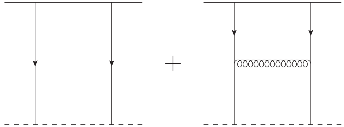
To calculate $V^{QQ}(r)$ using AdS/CFT we notice that now both strings attached to the quarks have to have the same orientation. Therefore the hanging string configuration from the left panel of Fig. 2 is now impossible, and the potential is given by the straight-strings configuration shown in Fig. 14. Just as for the $Q\bar{Q}$ system, the left panel in Fig. 14 gives zero contribution to the potential after renormalization and subtraction of self-interactions. We are left with the right panel in Fig. 14. Note that now both strings are oriented in the same direction, and can be parametrized as (cf. Eq. (27))

\displaystyle X_{1}^{M}=(\tau,{\vec{r}},z=\sigma),\ \ \ \ \ X_{2}^{M}=(\tau,{\vec{0}},z=\sigma).

(121)

The effect of this difference is only felt by the 2-form field coupling to the string $X_{2}$ , which changes its sign, as follows from Eq. (70). Hence the action of the configuration in the right panel of Fig. 14 differs from that in Fig. 3 by the sign of the 2-form contribution. We therefore write for the momentum-space $QQ$ potential

	$\displaystyle V^{QQ}(q)\,$	$\displaystyle=\,V_{adj}^{\phi}(q)+V_{adj}^{t^{0}}(q)-V_{adj}^{B}(q)+{\tilde{V}}_{adj}^{G}(q)$
		$\displaystyle=\,\frac{\lambda}{2\,N_{c}^{2}}\,\int\limits_{0}^{1}\,\frac{dz}{z^{2}}\,\left[\varphi(q,z)+\frac{5}{3}\,{\gothfamily t}^{0}(q,z)-4\,z^{2}\,{\cal B}_{0z}(q,z)-{\cal A}(q,z)\right]$		(122)

and for the coordinate-space potential

\displaystyle V^{QQ}(r)\,=\,V_{adj}^{\phi}(r)+V_{adj}^{t^{0}}(r)-V_{adj}^{B}(r)+V_{adj}^{G}(r).

(123)

The right-hand-sides of Eqs. (122) and (123) contain terms given by the results of the above calculations of the contributions to the $Q\bar{Q}$ potential. The $QQ$ potential from Eq. (122) can be evaluated numerically using the above techniques and is plotted in Fig. 13 (upper line). It appears to be attractive, though somewhat weaker than the $Q\bar{Q}$ potential.

The large- $r\,T$ behavior of $V^{QQ}(r)$ is dominated by the graviton exchange, just like in the $Q\bar{Q}$ case:

\displaystyle V^{QQ}(r)\bigg|_{r\,T\gg 1}\,\approx\,V_{adj}^{G}(r)\bigg|_{r\,T\gg 1}\,\approx\,-\frac{\lambda}{2\,N_{c}^{2}}\,\frac{0.86\pm 0.03}{2\,\pi\,r}\,e^{-2.33\,\pi\,r\,T}.

(124)

The small- $r\,T$ limit is less straightforward to find. First of all, using Eqs. (52), (69), (89), and (110) in Eq. (123) yields

\displaystyle V^{QQ}(r)\bigg|_{r\,T\ll 1}\,=\,0\ \ \ \text{(in the leading--logarithmic approximation)}.

(125)

This result can be interpreted as follows. The large- $q$ asymptotics of the supergravity fields given by Eqs. (50), (68), (88), and Eq. (109), that we used in deriving the potential asymptotics in Eqs. (52), (69), (89), and (110) in Eq. (123) comes from the part of the EOM for those fields that is independent of the curvature of AdS₅. Hence this part of the string-string interactions is the same as in the flat space. In the flat space, however, we know that the interaction between the parallel strings oriented in the same direction should vanish since this would be a BPS system. In a way the zero of Eq. (125) provides a cross-check that we have properly accounted for all the relevant supergravity modes.

The zero on Eq. (125) only implies that the leading–logarithm terms containing $(1/r)\ln(1/r\,T)$ , which gave rise to the small- $r\,T$ potential (114) in the $Q\bar{Q}$ case, cancel among each other in the $QQ$ case. This does not imply that the $QQ$ potential actually goes to zero as $r\,T\rightarrow 0$ . To determine the correct $r\,T\rightarrow 0$ asymptotics of the $QQ$ potential we have to solve the EOM for the four relevant supergravity fields ( $\phi$ , $t^{0}$ , $B_{MN}$ , $h_{MN}$ ) at $T=0$ and integrate

\displaystyle V^{QQ}_{T=0}(q)\,=\,\frac{\lambda}{2\,N_{c}^{2}}\,\int\limits_{0}^{\infty}\,\frac{dz}{z^{2}}\,\left[\varphi_{T=0}(q,z)+\frac{5}{3}\,{\gothfamily t}^{0}_{T=0}(q,z)-4\,z^{2}\,{\cal B}_{0z}^{T=0}(q,z)-{\cal A}_{T=0}(q,z)\right].

(126)

Putting $z_{h}\rightarrow\infty$ in the dilaton EOM (33) yields

\displaystyle\varphi_{zz}-\frac{3}{z}\,\varphi_{z}-q^{2}\,\varphi=z,

(127)

with the solution

\displaystyle\varphi_{T=0}(q,z)\,=\,-z^{3}\,\left\{\frac{1}{3}+\frac{\pi}{2\,q\,z}\,\left[L_{2}(q\,z)-I_{2}(q\,z)\right]\right\}.

(128)

In arriving at Eq. (128) we have required that $\varphi(q,z=0)=0$ and that $\varphi$ does not diverge more than linearly in $z$ as $z\rightarrow\infty$ (see Eq. (50)). In Eq. (128), $L_{2}$ is the modified Struve function and $I_{2}$ is the modified Bessel function. Due to the linear divergence at large- $z$ , the contribution of $\varphi$ from Eq. (128) to the $QQ$ potential (126) is infinite: since we know that this infinity would cancel with contributions from other fields, we have to add those other contributions first before integrating the result over $z$ .

For the massive scalar $t^{0}$ the $T=0$ EOM in momentum-space is

\displaystyle{\gothfamily t}^{0}_{zz}-\frac{3}{z}\ {\gothfamily t}^{0}_{z}-q^{2}\,{\gothfamily t}^{0}\,-\frac{32}{z^{2}}\,{\gothfamily t}^{0}\,=\,z.

(129)

Imposing the boundary condition ${\gothfamily t}^{0}(q,z=0)=0$ and requiring that ${\gothfamily t}^{0}$ is no more than linearly divergent in $z$ as $z\rightarrow\infty$ (see Eq. (68)) we obtain the solution of Eq. (129)

\displaystyle{\gothfamily t}^{0}_{T=0}(q,z)\,=\,-\frac{z^{3}}{35}\ F\left(1;-\frac{3}{2},\frac{9}{2};\frac{q^{2}\,z^{2}}{4}\right)+\frac{\pi}{2\,q}\,z^{2}\,I_{6}(q\,z).

(130)

Here $F$ is the generalized hypergeometric function.

The zero-temperature EOM of motion for the 2-form field is

\displaystyle z^{2}\,{\cal B}^{\prime\prime}_{0z}+3\,z\,{\cal B}^{\prime}_{0z}-(15+q^{2}\,z^{2})\,{\cal B}_{0z}=z\ .

(131)

The series solution of this equation can be straightforwardly constructed (again imposing the same boundary conditions as for the scalars, with the exception that the 2-form field actually goes to zero as $z\rightarrow\infty$ , as follows from Eq. (88)). The summation of the series is more involved, but can be accomplished yielding

	$\displaystyle q\,{\cal B}_{0z}^{T=0}(q,z)\,=\,-\frac{2\,\pi\,i}{q\,z}\,I_{4}(q\,z)+\frac{1}{4\,q^{2}\,z^{2}}\,\bigg\{2\,\pi$	$\displaystyle\left[(8+q^{2}\,z^{2})\,I_{1}(q\,z)-4\,q\,z\,\left(1+2\,I_{2}(q\,z)\right)\right]\,Y_{4}(-i\,q\,z)$
		$\displaystyle+\pi\,q^{3}\,z^{3}\ G^{3\,0}_{2\,4}\left(-\frac{i\,q\,z}{2},\frac{1}{2}\bigg\|\begin{array}[]{cccc}&-\frac{5}{2},&0&\\ -2,&-1,&2,&-\frac{5}{2}\end{array}\right)\bigg\}$

where $G$ is the generalized Meijer $G$ -function. Despite several terms containing an $i$ on the right-hand-side, Eq. (4) gives a real-valued 2-form field.

Finally, the Einstein equations at $T=0$ , reduced to a single equation for ${\cal A}$ , read

\displaystyle z\,(3-q^{2}\,z^{2})\,{\cal A}_{z\,z}-3\,\left(1\,-q^{2}\,z^{2}\right)\,{\cal A}_{z}-q^{2}\,z\,\left[1-q^{2}\,z^{2}\right]\,{\cal A}\,=\,\frac{4}{3}\,q^{2}z^{4}\ .

(134)

This equation can be solved by series expansion similar to how it was done in the non-zero temperature case. However, the series can only be summed numerically. Instead we simply solve Eq. (134) numerically, requiring that ${\cal A}(q,z=0)=0$ and that ${\cal A}$ maps onto the asymptotics of Eq. (109) at large- $q\,z$ .

Numerical evaluation of the resulting $QQ$ potential at $T=0$ by the integration over $z$ of the sum of all four contributions following Eq. (126) yields

\displaystyle V^{QQ}_{T=0}(q)\,=\,(-0.7\pm 0.1)\,\frac{\lambda}{N_{c}^{2}}\frac{1}{q^{2}}.

(135)

The corresponding coordinate-space potential is

\displaystyle V^{QQ}(r)\bigg|_{r\,T\ll 1}\,=\,(-0.7\pm 0.1)\,\frac{\lambda}{N_{c}^{2}}\frac{1}{4\,\pi\,r}.

(136)

We see that the net $QQ$ potential at small- $r\,T$ is attractive. We also observe that it is finite in the $T\rightarrow 0$ limit, unlike the $Q\bar{Q}$ potential of Eq. (114), and does not require string–fluctuation corrections to remain finite in this limit.

5 Summary and outlook

We computed the adjoint quark–anti-quark potential, as well as the quark–quark potential in a SYM plasma. Both potentials are of order- $\lambda/N_{c}^{2}$ , and both are attractive. For comparison, notice that at weak coupling both potentials are also of order- $\lambda/N_{c}^{2}$ . Moreover, the adjoint $Q\bar{Q}$ potential is repulsive at weak coupling, and so is the the $QQ$ potential with the quarks in the $N_{c}^{2}-N_{c}$ representation. On the other hand, the $QQ$ potential in the $\bar{N}_{c}$ representation is attractive at weak coupling. It appears that all the potentials, regardless of whether they are repulsive or attractive, become attractive at large ’t Hooft coupling.

To interpret this result we use the suggestion of [13] that the electric modes can be singled out non-perturbatively by identifying the $CT$ -odd interaction channel. The quantum numbers of the supergravity fields contributing to the potentials calculated above can be found in [15] (see also [11] for a table of the quantum numbers of the relevant fields excluding $t^{0}$ ). We see that the dilaton, graviton, and $t^{0}$ are $CT$ -even, while $B_{0z}$ is $CT$ -odd. We can thus identify the 2-form contribution as corresponding to chromo-electric modes in the gauge theory. The remaining dilaton, massive scalar and the graviton may correspond to either magnetic modes, or to even numbers of electric mode exchanges. The latter are probably not very important in the mix, since the chromo-electric (2-form) contribution by itself is smaller than the sum of all other contributions: hence it is likely that the scalars and the dilaton correspond mainly to the chromo-magnetic modes on the boundary. The chromo-electric (2-form) contribution changes sign in going from $Q\bar{Q}$ to $QQ$ , which seems natural for the chromo-electric modes. In the perturbative weak-coupling limit, when the potentials are calculated at lowest order by two-gluon exchanges between Polyakov loops [18], the interaction is entirely due to chromo-electric modes. However, even at weak coupling it appears that the chromo-magnetic modes are less screened than the chromo-electric ones, though they do not couple directly to the heavy quark and anti-quark, and their contribution is suppressed by extra powers of the coupling coming from the loop diagrams needed to couple them to the quarks [45, 13]. It seems that our above results suggest that at strong coupling the magnetic modes dominate over electric modes in the $Q\bar{Q}$ and $QQ$ potentials, making both of them attractive. The fact the the leading pole for the graviton is smaller than the leading pole for the 2-form field can be interpreted as magnetic modes being less screened even in the strong coupling limit. Small-coupling suppression of the magnetic contribution’s coupling to the static heavy quarks by higher orders of the coupling is no longer an issue at strong coupling. Thus it seems natural that magnetic modes dominate at strong coupling (since they are screened less than electric modes and couple to quarks similarly) making both potentials attractive.

For the adjoint $Q\bar{Q}$ potential (and for the $QQ$ potential in the $N_{c}^{2}-N_{c}$ representation) we thus conjecture that in transition from weak to strong coupling the potential, while remaining of order- $\lambda/N_{c}^{2}$ , would change its sign. There should be no change of sign for the $QQ$ potential in the $\bar{N}_{c}$ representation.

In [11] the Debye screening mass was identified as the leading pole in the $CT$ -odd channel. Of all the $CT$ -odd supergravity particles, the one with the lowest location of the pole on imaginary axis is the axion [15], the EOM and, therefore, poles for which are the same as for the dilaton considered above. The authors of [15] have therefore identified $m_{D}=3.4041\,\pi\,T$ as the Debye mass of ${\cal N}=4$ SYM plasma. However, it may seem a little peculiar that the axion does not couple to the string world-sheet at the leading (tree-level) order: how can electric modes in gauge theory not couple to a static heavy quark? It is possible (though seems a little hard to determine precisely) that the single axion can still couple to the string through some higher-order diagrams, with the axion-string coupling suppressed by additional powers of $1/N_{c}^{2}$ . If that was the case, the $CT$ -odd part of the $Q\bar{Q}$ potential at large- $rT$ would be proportional to

\displaystyle\frac{\lambda}{N_{c}^{2}}\,e^{-5.1085\,\pi\,r\,T}+O\left(\frac{1}{N_{c}^{6}}\right)\,e^{-3.4041\,\pi\,r\,T}.

(137)

Indeed at very large distances, parametrically defined by $r\,T\gg\ln N_{c}^{2}$ , the axion would dominate, with its mass being the correct Debye mass. It appears that more work is needed in order to determine the degree of suppression of a single-axion coupling to the string world-sheet and to eliminate the possibility of this coupling being zero. If the coupling is in fact zero, the leading pole of the 2-form field at $5.1085\,\pi\,T$ would be the correct Debye mass. We leave this for future work.

Other possible future improvements of our result may include performing similar calculations of the $Q\bar{Q}$ and $QQ$ potential in more QCD-like geometries [46, 47, 48, 49, 50, 51, 52, 53, 54, 55, 56, 57]. Indeed the positions of the poles and the corresponding residues would be modified by the new geometries, along with other calculational details. One may even include finite quark masses (which are infinite in our present calculation) by inserting a probe D7-brane wrapped over $S^{5}$ along the lines of [58] and having the strings dual to the quarks end on this D7 brane. After performing a more QCD-like calculations, one may hope to be able to perform a meaningful comparison of the results to the lattice QCD data [26, 27].

Acknowledgments.

The authors are grateful to Dick Furnstahl, Samir Mathur, Jorge Noronha, Misha Stephanov, Chung-I Tan, Diana Vaman, and Larry Yaffe for very informative discussions. We would like to especially thank Dick Furnstahl for the help with the numerical solution, and Samir Mathur and Chung-I Tan for discussions of their work [15]. This research is sponsored in part by the U.S. Department of Energy under Grant No. DE-SC0004286.

Appendix A Solution of Einstein equations with a straight string as a source

Linearized Einstein equations (94) for the metric (90) read


$\displaystyle(t\,t)\hskip 28.45274pt$	$\displaystyle 8\,{\cal B}+z\,(1+z^{4})\,(3{\cal A}_{z}-{\cal B}_{z})+2\,z\,(2+z^{4})\,{\gothfamily h}_{z}-z^{2}\,(1-z^{4})\,{\gothfamily h}_{z\,z}+q^{2}\,z^{2}\,{\gothfamily h}\,=\,-\frac{2}{3}\,z^{3}$	(A1a)
$\displaystyle(r\,r)\hskip 28.45274pt$	$\displaystyle 8\,{\cal B}+z\left[2\,(3-z^{4})\,{\cal A}_{z}-(1-z^{4})\,{\cal B}_{z}+(1-z^{4})\,{\gothfamily h}_{z}-z\,(1-z^{4})\,{\cal A}_{z\,z}+z\,q^{2}\,{\cal A}\right.$
	$\displaystyle\hskip 142.26378pt\left.-z\,r\,\partial_{r}^{2}\,({\cal A}+{\cal B}+{\gothfamily h})\right]\,=\,\frac{4}{3}\,z^{3}$	(A1b)
$\displaystyle(\theta\,\theta)\hskip 28.45274pt$	$\displaystyle 8\,{\cal B}+z\left[2\,(3-z^{4})\,{\cal A}_{z}-(1-z^{4})\,{\cal B}_{z}+(1-z^{4})\,{\gothfamily h}_{z}-z\,(1-z^{4})\,{\cal A}_{z\,z}+z\,q^{2}\,{\cal A}\right.$
	$\displaystyle\hskip 142.26378pt\left.-z\,\partial_{r}\,({\cal A}+{\cal B}+{\gothfamily h})\right]\,=\,\frac{4}{3}\,z^{3}$	(A1c)
$\displaystyle(z\,z)\hskip 28.45274pt$	$\displaystyle 8\,{\cal B}+z\left[3\,(1+z^{4})\,{\cal A}_{z}-2\,(2-z^{4})\,{\cal B}_{z}+(1+5\,z^{4})\,{\gothfamily h}_{z}-3\,z\,(1-z^{4})\,{\cal A}_{z\,z}-z\,(1-z^{4})\,{\gothfamily h}_{z\,z}\right.$
	$\displaystyle\hskip 142.26378pt\left.+\,z\,q^{2}\,{\cal B}\,\right]\,=\,-\frac{2}{3}\,z^{3}$	(A1d)

where we have omitted the $\phi\,\phi$ and $r\,z$ components, which follow from the equations given above. As usual ${\cal A}_{z}=\partial_{z}{\cal A}$ and ${\cal A}_{z\,z}=\partial_{z}^{2}{\cal A}$ .

Note that it appears difficult to perform Fourier transform on the $r\,r$ and $\theta\,\theta$ components, since, for our $\theta$ - and $\phi$ -independent metric in spherical coordinates not all $r$ -derivatives in those equations lead to powers of $q$ in an obvious way. That is why we have, perhaps a bit sloppily, left some powers of $r$ and $\partial_{r}$ in those two equations: these object should be understood now as some operators in $q$ -space. Subtracting $r\,r$ and $\theta\,\theta$ equations from each other, and transforming the result back into coordinate space, we get

\displaystyle-r\,\partial_{r}^{2}\,(\bar{A}+\bar{B}+\bar{h})+\partial_{r}\,(\bar{A}+\bar{B}+\bar{h})\,=\,0

(A2)

which implies that

\displaystyle\bar{A}+\bar{B}+\bar{h}\,=\,\rho_{1}(z)\,r^{2}+\rho_{2}(z)

(A3)

with $\rho_{1}(z)$ and $\rho_{2}(z)$ some arbitrary functions of $z$ . On the physical grounds one may require that the metric should fall off with increasing $r$ at large- $r$ : this would put $\rho_{1}$ and $\rho_{2}$ to zero. Alternatively one can show that, employing the residual diffeomorphism invariance left in the metric ansatz (90) one can eliminate $\rho_{1}(z)$ and $\rho_{2}(z)$ , obtaining Eq. (97), which in momentum space leads to

\displaystyle{\cal A}+{\cal B}+{\gothfamily h}\,=\,0.

(A4)

Using Eq. (A4) to eliminate ${\gothfamily h}$ from Eqs. (A1), and subtracting $z\,z$ equation from $t\,t$ , we write


$\displaystyle(t\,t)-(z\,z)\hskip 28.45274pt$	$\displaystyle-3\,(1-z^{4})\,{\cal A}_{z}+3\,z\,(1-z^{4})\,{\cal A}_{z\,z}-z\,q^{2}\,{\cal A}-2\,z\,q^{2}\,{\cal B}\,=\,0$	(A5a)
$\displaystyle(r\,r)\hskip 28.45274pt$	$\displaystyle 8\,{\cal B}+z\left[(5-z^{4})\,{\cal A}_{z}-2\,(1-z^{4})\,{\cal B}_{z}-z\,(1-z^{4})\,{\cal A}_{z\,z}+z\,q^{2}\,{\cal A}\right]\,=\,\frac{4}{3}\,z^{3},$	(A5b)

which is now written entirely in momentum space. Solving Eq. (A5a) for ${\cal B}$ yields

\displaystyle{\cal B}\,=\,-\frac{1}{2\,z\,q^{2}}\,\left[3\,(1-z^{4})\,({\cal A}_{z}-z\,{\cal A}_{z\,z})+z\,q^{2}\,{\cal A}\right].

(A6)

Substituting Eq. (A6) into Eq. (A5b) yields a 3rd-order differential equation for ${\cal A}$ . Solving this equation to express ${\cal A}_{z\,z\,z}$ in terms of lower-order derivatives of ${\cal A}$ , we can use the result, along with Eqs. (A4) and (A6), in, say, Eq. (A1a) to obtain Eq. (98) in the text (after some considerable algebra).

References

[1] J. M. Maldacena, Wilson loops in large N field theories, Phys. Rev. Lett. 80 (1998) 4859–4862, [hep-th/9803002].
[2] S.-J. Rey and J.-T. Yee, Macroscopic strings as heavy quarks in large N gauge theory and anti-de Sitter supergravity, Eur. Phys. J. C22 (2001) 379–394, [hep-th/9803001].
[3] J. M. Maldacena, The large N limit of superconformal field theories and supergravity, Adv. Theor. Math. Phys. 2 (1998) 231–252, [hep-th/9711200].
[4] S. S. Gubser, I. R. Klebanov, and A. M. Polyakov, Gauge theory correlators from non-critical string theory, Phys. Lett. B428 (1998) 105–114, [hep-th/9802109].
[5] E. Witten, Anti-de sitter space and holography, Adv. Theor. Math. Phys. 2 (1998) 253–291, [hep-th/9802150].
[6] E. Witten, Anti-de Sitter space, thermal phase transition, and confinement in gauge theories, Adv. Theor. Math. Phys. 2 (1998) 505–532, [hep-th/9803131].
[7] O. Aharony, S. S. Gubser, J. M. Maldacena, H. Ooguri, and Y. Oz, Large N field theories, string theory and gravity, Phys. Rept. 323 (2000) 183–386, [hep-th/9905111].
[8] S.-J. Rey, S. Theisen, and J.-T. Yee, Wilson-Polyakov loop at finite temperature in large N gauge theory and anti-de Sitter supergravity, Nucl. Phys. B527 (1998) 171–186, [hep-th/9803135].
[9] A. Brandhuber, N. Itzhaki, J. Sonnenschein, and S. Yankielowicz, Wilson loops in the large N limit at finite temperature, Phys. Lett. B434 (1998) 36–40, [hep-th/9803137].
[10] D. J. Gross and H. Ooguri, Aspects of large N gauge theory dynamics as seen by string theory, Phys. Rev. D58 (1998) 106002, [hep-th/9805129].
[11] D. Bak, A. Karch, and L. G. Yaffe, Debye screening in strongly coupled N=4 supersymmetric Yang-Mills plasma, JHEP 08 (2007) 049, [arXiv:0705.0994].
[12] O. Aharony and E. Witten, Anti-de Sitter space and the center of the gauge group, JHEP 11 (1998) 018, [hep-th/9807205].
[13] P. B. Arnold and L. G. Yaffe, The NonAbelian Debye screening length beyond leading order, Phys. Rev. D52 (1995) 7208–7219, [hep-ph/9508280].
[14] C. Csaki, H. Ooguri, Y. Oz, and J. Terning, Glueball mass spectrum from supergravity, JHEP 01 (1999) 017, [hep-th/9806021].
[15] R. C. Brower, S. D. Mathur, and C.-I. Tan, Glueball Spectrum for QCD from AdS Supergravity Duality, Nucl. Phys. B587 (2000) 249–276, [hep-th/0003115].
[16] J. L. Albacete, Y. V. Kovchegov, and A. Taliotis, Heavy Quark Potential at Finite Temperature in AdS/CFT Revisited, Phys. Rev. D78 (2008) 115007, [arXiv:0807.4747].
[17] L. D. McLerran and B. Svetitsky, Quark Liberation at High Temperature: A Monte Carlo Study of SU(2) Gauge Theory, Phys. Rev. D24 (1981) 450.
[18] S. Nadkarni, Nonabelian Debye Screening. 1. The Color Averaged Potential, Phys. Rev. D33 (1986) 3738.
[19] C. Gale and J. I. Kapusta, MODIFICATION OF DEBYE SCREENING IN GLUON PLASMA, Phys. Lett. B198 (1987) 89–91.
[20] M. Laine, O. Philipsen, P. Romatschke, and M. Tassler, Real-time static potential in hot QCD, JHEP 03 (2007) 054, [hep-ph/0611300].
[21] N. Brambilla, J. Ghiglieri, A. Vairo, and P. Petreczky, Static quark-antiquark pairs at finite temperature, Phys. Rev. D78 (2008) 014017, [arXiv:0804.0993].
[22] Y. Burnier, M. Laine, and M. Vepsalainen, Dimensionally regularized Polyakov loop correlators in hot QCD, JHEP 01 (2010) 054, [arXiv:0911.3480].
[23] R. Baier and O. K. Kalashnikov, The NonAbelian screening potential beyond the leading order, Phys. Lett. B328 (1994) 450–456, [hep-ph/9402361].
[24] S. Peigne and S. M. H. Wong, NonDebye screening in high temperature QCD, Phys. Lett. B346 (1995) 322–328, [hep-ph/9406276].
[25] A. Taliotis, $q{\bar{q}}$ Potential at Finite T and Weak Coupling in ${\cal N}=4$ , arXiv:1011.6618.
[26] A. Bazavov, P. Petreczky, and A. Velytsky, Quarkonium at Finite Temperature, arXiv:0904.1748.
[27] P. Petreczky, Heavy quark potentials and quarkonia binding, Eur. Phys. J. C43 (2005) 51–57, [hep-lat/0502008].
[28] N. Brambilla, J. Ghiglieri, P. Petreczky, and A. Vairo, Polyakov loop and correlator of Polyakov loops at next-to- next-to-leading order, Phys. Rev. D82 (2010) 074019, [arXiv:1007.5172].
[29] D. E. Berenstein, R. Corrado, W. Fischler, and J. M. Maldacena, The operator product expansion for Wilson loops and surfaces in the large N limit, Phys. Rev. D59 (1999) 105023, [hep-th/9809188].
[30] U. H. Danielsson, E. Keski-Vakkuri, and M. Kruczenski, Vacua, Propagators, and Holographic Probes in AdS/CFT, JHEP 01 (1999) 002, [hep-th/9812007].
[31] R. A. Janik and R. B. Peschanski, High energy scattering and the AdS/CFT correspondence, Nucl. Phys. B565 (2000) 193–209, [hep-th/9907177].
[32] L. D. McLerran and B. Svetitsky, A Monte Carlo Study of SU(2) Yang-Mills Theory at Finite Temperature, Phys. Lett. B98 (1981) 195.
[33] H. J. Kim, L. J. Romans, and P. van Nieuwenhuizen, The Mass Spectrum of Chiral N=2 D=10 Supergravity on S**5, Phys. Rev. D32 (1985) 389.
[34] G. Arutyunov and S. Frolov, Some cubic couplings in type IIB supergravity on AdS(5) x S(5) and three-point functions in SYM(4) at large N, Phys. Rev. D61 (2000) 064009, [hep-th/9907085].
[35] G. Arutyunov and S. Frolov, Scalar quartic couplings in type IIB supergravity on AdS(5) x S(5), Nucl. Phys. B579 (2000) 117–176, [hep-th/9912210].
[36] S. Lee, S. Minwalla, M. Rangamani, and N. Seiberg, Three-point functions of chiral operators in D = 4, N = 4 SYM at large N, Adv. Theor. Math. Phys. 2 (1998) 697–718, [hep-th/9806074].
[37] M. Zyskin, A note on the glueball mass spectrum, Phys. Lett. B439 (1998) 373–381, [hep-th/9806128].
[38] R. C. Brower, S. D. Mathur, and C.-I. Tan, Discrete spectrum of the graviton in the AdS(5) black hole background, Nucl. Phys. B574 (2000) 219–244, [hep-th/9908196].
[39] N. R. Constable and R. C. Myers, Spin-two glueballs, positive energy theorems and the AdS/CFT correspondence, JHEP 10 (1999) 037, [hep-th/9908175].
[40] R. de Mello Koch, A. Jevicki, M. Mihailescu, and J. P. Nunes, Evaluation Of Glueball Masses From Supergravity, Phys. Rev. D58 (1998) 105009, [hep-th/9806125].
[41] J. J. Friess, S. S. Gubser, G. Michalogiorgakis, and S. S. Pufu, The stress tensor of a quark moving through N = 4 thermal plasma, Phys. Rev. D75 (2007) 106003, [hep-th/0607022].
[42] S. Lin and E. Shuryak, Stress Tensor of Static Dipoles in strongly coupled $\cal{N}$ =4 Gauge Theory, Phys. Rev. D76 (2007) 085014, [arXiv:0707.3135].
[43] P. M. Chesler and L. G. Yaffe, The stress-energy tensor of a quark moving through a strongly-coupled N=4 supersymmetric Yang-Mills plasma: comparing hydrodynamics and AdS/CFT, arXiv:0712.0050.
[44] J. K. Erickson, G. W. Semenoff, R. J. Szabo, and K. Zarembo, Static potential in N = 4 supersymmetric Yang-Mills theory, Phys. Rev. D61 (2000) 105006, [hep-th/9911088].
[45] E. Braaten and A. Nieto, Asymptotic behavior of the correlator for Polyakov loops, Phys. Rev. Lett. 74 (1995) 3530–3533, [hep-ph/9410218].
[46] J. Polchinski and M. J. Strassler, Hard scattering and gauge / string duality, Phys. Rev. Lett. 88 (2002) 031601, [hep-th/0109174].
[47] H. Boschi-Filho and N. R. F. Braga, Gauge/string duality and scalar glueball mass ratios, JHEP 05 (2003) 009, [hep-th/0212207].
[48] J. Erlich, E. Katz, D. T. Son, and M. A. Stephanov, QCD and a Holographic Model of Hadrons, Phys. Rev. Lett. 95 (2005) 261602, [hep-ph/0501128].
[49] L. Da Rold and A. Pomarol, Chiral symmetry breaking from five dimensional spaces, Nucl. Phys. B721 (2005) 79–97, [hep-ph/0501218].
[50] H. Boschi-Filho, N. R. F. Braga, and H. L. Carrion, Glueball Regge trajectories from gauge/string duality and the Pomeron, Phys. Rev. D73 (2006) 047901, [hep-th/0507063].
[51] H. R. Grigoryan and A. V. Radyushkin, Form Factors and Wave Functions of Vector Mesons in Holographic QCD, Phys. Lett. B650 (2007) 421–427, [hep-ph/0703069].
[52] A. Karch, E. Katz, D. T. Son, and M. A. Stephanov, Linear Confinement and AdS/QCD, Phys. Rev. D74 (2006) 015005, [hep-ph/0602229].
[53] A. Karch, E. Katz, D. T. Son, and M. A. Stephanov, On the sign of the dilaton in the soft wall models, arXiv:1012.4813.
[54] H. R. Grigoryan and A. V. Radyushkin, Structure of Vector Mesons in Holographic Model with Linear Confinement, Phys. Rev. D76 (2007) 095007, [arXiv:0706.1543].
[55] O. Andreev and V. I. Zakharov, On Heavy-Quark Free Energies, Entropies, Polyakov Loop, and AdS/QCD, JHEP 04 (2007) 100, [hep-ph/0611304].
[56] O. Andreev, Renormalized Polyakov Loop in the Deconfined Phase of SU(N) Gauge Theory and Gauge/String Duality, Phys. Rev. Lett. 102 (2009) 212001, [arXiv:0903.4375].
[57] S. He, M. Huang, and Q.-S. Yan, Logarithmic correction in the deformed ${\rm AdS}_{5}$ model to produce the heavy quark potential and QCD beta function, Phys. Rev. D83 (2011) 045034, [arXiv:1004.1880].
[58] A. Karch and E. Katz, Adding flavor to AdS/CFT, JHEP 06 (2002) 043, [hep-th/0205236].

Gravity Dual Corrections to the Heavy Quark Potential at Finite-Temperature

Abstract:

Keywords:

1 Introduction

2 Two definitions of the heavy quark potential at finite temperature

2.1 Singlet and octet potentials

2.2 One unified potential

3 The adjoint contribution to the Q​Q¯Q\bar{Q} potential

3.1 The Dilaton

3.1.1 Dilaton potential and the EOM

3.1.2 Solution of the dilaton EOM

3.1.3 Asymptotics of the dilaton contribution

3.2 Massive Scalars

3.2.1 The potential and EOM

3.2.2 Solution of the EOM for t0t^{0}

3.2.3 Asymptotics of the massive scalar contribution

3.3 Two-Form Fields

3.3.1 The potential and EOM

3.3.2 Solution of the 2-form EOM

3.3.3 Asymptotics of the 2-form contribution

3.4 The Graviton

3.4.1 The potential and Einstein equations

3.4.2 Solution of Einstein equations

3.4.3 Asymptotics of the graviton contribution

3.5 The Net Result

4 The Q​QQQ potential

5 Summary and outlook

Acknowledgments.

Appendix A Solution of Einstein equations with a straight string as a source

References

3 The adjoint contribution to the $Q\bar{Q}$ potential

3.2.2 Solution of the EOM for $t^{0}$

4 The $QQ$ potential