跳到论文正文
W Papers独立论文阅读器 arXiv:1105.2282 论文正文 计算阅读时间 · 0%
引用这篇论文根据当前论文元数据生成,正式投稿前建议核对。


License: arXiv.org perpetual non-exclusive license
arXiv:1105.2282v2 [quant-ph] 21 Nov 2011

Average output entropy for quantum channels

Christopher King    David K. Moser1: Department of Mathematics2: Department of PhysicsNortheastern UniversityBoston MA 02115
Abstract

We study the regularized average Renyi output entropy S¯rreg\overline{S}_{r}^{\mathrm{reg}} of quantum channels. This quantity gives information about the average noisiness of the channel output arising from a typical, highly entangled input state in the limit of infinite dimensions. We find a closed expression for βrreg\beta_{r}^{\mathrm{reg}}, a quantity which we conjecture to be equal to S¯rreg\overline{S}_{r}^{\mathrm{reg}}. We find an explicit form for βrreg\beta_{r}^{\mathrm{reg}} for some entanglement-breaking channels, and also for the qubit depolarizing channel Δλ\Delta_{\lambda} as a function of the parameter λ\lambda. We prove equality of the two quantities in some cases, in particular we conclude that for Δλ\Delta_{\lambda} both are non-analytic functions of the variable λ\lambda.

1 Introduction

The noisiness of a quantum channel is closely related to its ability to transfer information, and is reflected in the values of the various channel capacities. Much work has been done on understanding the capacities, for example [1] provides a recent survey. These capacities are sometimes difficult to analyze directly, for example the Holevo capacity is computed using multiple output states. Accordingly other more mathematically tractable quantities have been used to measure the amount of noise introduced by the channel. One example is the minimal output Renyi entropy [2] of a channel 𝒜{\cal A}, defined for r≥1r\geq 1:

Sr,min​(𝒜)=min|ϕ⟩⁡11−r​log​Tr​(𝒜⁡(|ϕ⟩​⟨ϕ|))rS_{r,\min}(\mathcal{A})=\min_{|\phi\rangle}\,\frac{1}{1-r}\,\log\mathrm{Tr\,}\left(\mathcal{A}(|\phi\rangle\langle\phi|)\right)^{r}

At r=1r=1 this yields the minimal output von Neumann entropy, which has a close connection to the classical capacity of the channel [3]. The entropies for r>1r>1 also provide useful properties of the channel, and in some cases are easier to analyze and compute. The famous additivity conjecture concerns the regularized version of this quantity, which is defined as

Sr,minreg​(𝒜)=limn→∞1n​Sr,min​(𝒜⊗n)S_{r,\min}^{\mathrm{reg}}(\mathcal{A})=\lim_{n\rightarrow\infty}\,\frac{1}{n}\,S_{r,\min}(\mathcal{A}^{\otimes n})

(the existence of the limit is an easy consequence of the sub-additivity bound 𝒮r,min​(𝒜⊗ℬ)≤𝒮r,min​(𝒜)+𝒮r,min​(ℬ){\cal S}_{r,\min}({\cal A}\otimes{\cal B})\leq{\cal S}_{r,\min}({\cal A})+{\cal S}_{r,\min}({\cal B})). While the inequality Sr,minreg​(𝒜)≤Sr,min​(𝒜)S_{r,\min}^{\mathrm{reg}}(\mathcal{A})\leq S_{r,\min}(\mathcal{A}) is always true, it was an open question for several years whether equality holds. It is now known that equality does not hold in general [4, 5], so this raises the interesting question of determining Sr,minreg​(𝒜)S_{r,\min}^{\mathrm{reg}}(\mathcal{A}). Except for those channels where additivity does hold, the value of this regularized quantity is unknown. For channels with non-additive Holevo capacity the classical capacity is also defined by such a regularized quantity, so it is an important problem to find new ways to calculate these regularized limits. In a sense we follow a strategy opposite to the random channel methods used to disprove the additivity conjecture; our high-dimensional channels are products of fixed channels, and thus are constructed explicitly.

In the hopes of finding some new insights into these regularized channel properties we consider a related quantity which also measures the noisiness of the channel, namely the average output Renyi entropy. This measures the entropy of the channel output for typical input states, rather than the smallest value which is used to compute the minimal output entropy. For a finite-dimensional channel this is defined for all r≥1r\geq 1 by

S¯r​(𝒜)=𝔼⁡[11−r​log⁡Tr​(𝒜⁡(|ϕ⟩​⟨ϕ|))r]\overline{S}_{r}(\mathcal{A})=\mathrm{\mathbb{E}}\left[\frac{1}{1-r}\,\log\mathrm{Tr\,}\left(\mathcal{A}(|\phi\rangle\langle\phi|)\right)^{r}\right]

where the expectation is computed using the uniform probability measure on the set of input pure states. We also consider the related quantity

βr​(𝒜)=11−r​log⁡𝔼⁡[Tr​(𝒜⁡(|ϕ⟩​⟨ϕ|))r]\beta_{r}(\mathcal{A})=\,\frac{1}{1-r}\,\log\mathrm{\mathbb{E}}\left[\mathrm{Tr\,}\left(\mathcal{A}(|\phi\rangle\langle\phi|)\right)^{r}\right]

Note that by Jensen’s inequality

S¯r​(𝒜)≥βr​(𝒜).\overline{S}_{r}(\mathcal{A})\geq\beta_{r}(\mathcal{A})\,. (1)

These quantities can be computed (at least numerically) for any given channel. In operational terms, they describe the long-run average output Renyi entropy of the channel for a sequence of random pure input states. Loosely speaking, they measure the average noisiness of an output state from the channel.

As with the minimal Renyi entropy, we also consider the regularized versions of these quantities. However unlike the minimal Renyi entropy, the existence of these regularized limits is not obvious, so we define them conservatively using the lim inf\liminf:

S¯rreg​(𝒜)\displaystyle\overline{S}_{r}^{\mathrm{reg}}(\mathcal{A}) =lim infn→∞1n​S¯r​(𝒜⊗n)\displaystyle=\liminf_{n\rightarrow\infty}\,\frac{1}{n}\,\overline{S}_{r}(\mathcal{A}^{\otimes n}) (2)
βrreg​(𝒜)\displaystyle\beta_{r}^{\mathrm{reg}}(\mathcal{A}) =lim infn→∞1n​βr​(𝒜⊗n)\displaystyle=\liminf_{n\rightarrow\infty}\,\frac{1}{n}\,\beta_{r}(\mathcal{A}^{\otimes n})

We conjecture that the two quantities in (2) are equal, however we do not yet have a proof of this for a general channel. For the specific channels we look at in more detail the quantity βrreg​(𝒜)\beta_{r}^{{\rm reg}}({\cal A}) is given by the expression above with lim inf\liminf replaced by lim\lim. But from the closed expression for βrreg​(𝒜)\beta_{r}^{\mathrm{reg}}(\mathcal{A}) presented below there is a possibility for more complex limiting behavior.

For one special class of channels we can compute a simple formula for βrreg​(𝒜)\beta_{r}^{\mathrm{reg}}(\mathcal{A}) for integer values of rr. These are a subset of the entanglement breaking (E-B) channels [6, 7], which can be written in the form 𝒜⁡(ρ)=∑kσk​Tr​(Xk​ρ){\cal A}(\rho)=\sum_{k}\sigma_{k}\mathrm{Tr\,}(X_{k}\rho) – for some states σk{\sigma_{k}} and with XkX_{k} a POVM – meeting the additional condition Tr⁡(∏i=1rσki)≥0\mathrm{Tr}\left(\prod_{i=1}^{r}\sigma_{k_{i}}\right)\geq 0. For r=2r=2 this includes all the E-B channels. For higher rr a particular class of E-B channels that fulfill the condition are the QC channels as defined by Holevo [8], where σk=|k⟩​⟨k|\sigma_{k}=|k\rangle\langle k| are pure states formed by an orthonormal basis. For unital E-B channels which satisfy the condition on the σk\sigma_{k} we can prove even more, namely that S¯rreg​(𝒜)\overline{S}_{r}^{\mathrm{reg}}(\mathcal{A})=βrreg​(𝒜)\beta_{r}^{\mathrm{reg}}(\mathcal{A}) = log⁡d\log d.

We consider only finite-dimensional channels with equal input and output dimensions, and we define the dimension of the channel to be this common value. The identity matrix is denoted by 𝟙\mathbbm{1}.

Theorem 1 (proof in 2.5).
  • (a)

    Let r≥2r\geq 2 be an integer, and 𝒜⁡(ρ)=∑σk​Tr​(Xk​ρ)\mathcal{A}(\rho)=\sum\sigma_{k}\mathrm{Tr}\left(X_{k}\rho\right) an entanglement breaking channel satisfying the condition Tr⁡(∏i=1rσki)≥0\mathrm{Tr}\left(\prod_{i=1}^{r}\sigma_{k_{i}}\right)\geq 0 for all choices of {ki}\{k_{i}\}. Then

    βrreg​(𝒜)=limn→∞1n​βr​(𝒜⊗n)=11−r​log⁡Tr⁡(𝒜​(𝟙/d)r).\beta_{r}^{\mathrm{reg}}(\mathcal{A})=\lim_{n\to\infty}\frac{1}{n}\beta_{r}(\mathcal{A}^{\otimes n})=\frac{1}{1-r}\log\mathrm{Tr\,}({\cal A}(\mathbbm{1}/d)^{r})\,.
  • (b)

    Let 𝒜{\cal A} be a d-dimensional unital entanglement-breaking channel, 𝒜⁡(𝟙)=𝟙\mathcal{A}(\mathbbm{1})=\mathbbm{1}, satisfying the condition Tr⁡(∏i=1mσki)\mathrm{Tr}\left(\prod_{i=1}^{m}\sigma_{k_{i}}\right) for all integer m≥2m\geq 2. Then for all real r≥1r\geq 1

    S¯rreg​(𝒜)=βrreg​(𝒜)=log⁡d.\overline{S}_{r}^{\mathrm{reg}}(\mathcal{A})=\beta_{r}^{\mathrm{reg}}(\mathcal{A})=\log d\,.

We also derive an explicit expression for βrreg​(𝒜)\beta_{r}^{\mathrm{reg}}(\mathcal{A}) in the general case. The statement of this result requires some additional notation. First recall the definition of the Choi-Jamiolkowski representation [9] of a channel, namely

C​h​o​i​(𝒜)=∑x,y𝒜⁡(|x⟩​⟨y|)⊗|x⟩​⟨y|Choi({\cal A})=\sum_{x,y}{\cal A}(|x\rangle\langle y|)\otimes|x\rangle\langle y|

where |x⟩|x\rangle and |y⟩|y\rangle are orthonormal bases of pure input states. Also let S​y​m​(r)Sym(r) denote the symmetric group on rr letters. Then every element α∈S​y​m​(r)\alpha\in Sym(r) defines a permutation operator on (ℂd)⊗r(\mathbb{C}^{d})^{\otimes r} by ℛ(α)(v1⊗⋯⊗vr)=vα⁡(1)⊗⋯⊗vα⁡(r){\cal R}(\alpha)(v_{1}\otimes\cdots\otimes v_{r})=v_{\alpha(1)}\otimes\cdots\otimes v_{\alpha(r)}.

Definition 2.

Let 𝒜{\cal A} be a channel. For all α∈S​y​m​(r)\alpha\in Sym(r) define

𝒬𝒜,r​(α)=Tr⁡[C​h​o​i​(𝒜)⊗r​(ℛ⁡(123​…​r)⊗ℛ⁡(α))].\mathcal{Q}_{{\cal A},\,r}(\alpha)=\mathrm{Tr\,}\left[Choi({\cal A})^{\otimes r}({\cal R}(123\dots r)\otimes{\cal R}(\alpha))\right]\,. (3)

Furthermore, for some channels βrreg\beta_{r}^{\mathrm{reg}} is a simple limit. One such class are the entrywise positive maps defined studied in [10].

Definition 3.

A channel 𝒜\mathcal{A} is called entrywise positive if there exist a bases for input and output space such that ⟨s|𝒜⁡(|x⟩​⟨y|)|t⟩≥0\langle s|\mathcal{A}(|x\rangle\langle y|)|t\rangle\geq 0 for all x,y,s,tx,y,s,t.

It is clear that this definition is equivalent to C​h​o​i​(𝒜)Choi(\mathcal{A}) being entrywise positive.

Theorem 4 (proof in 2.4).
  • (a)

    Let r≥2r\geq 2 be an integer and let 𝒬max=maxα∈S​y​m​(r)⁡|𝒬𝒜,r​(α)|\mathcal{Q}_{\max}=\max_{\alpha\in Sym(r)}|\mathcal{Q}_{{\cal A},\,r}(\alpha)|. Then

    βrreg​(𝒜)=r​log⁡d−log⁡𝒬maxr−1.\beta_{r}^{\mathrm{reg}}(\mathcal{A})=\frac{r\log d-\log\mathcal{Q}_{\max}}{r-1}\,.
  • (b)

    Let r≥2r\geq 2 be an integer. If the maximum 𝒬max\mathcal{Q}_{\mathrm{max}} is attained for a unique α\alpha then the lim inf\liminf in βrreg\beta_{r}^{\mathrm{reg}} can be replaced with a regular limit:

    βrreg​(𝒜)=limn→∞1n​βr​(𝒜⊗n).\beta_{r}^{\mathrm{reg}}(\mathcal{A})=\lim_{n\to\infty}\frac{1}{n}\beta_{r}(\mathcal{A}^{\otimes n})\,.
  • (c)

    If the channel 𝒜\mathcal{A} is entrywise positive then for all integer r≥2r\geq 2

    βrreg​(𝒜)=limn→∞1n​βr​(𝒜⊗n).\beta_{r}^{\mathrm{reg}}(\mathcal{A})=\lim_{n\to\infty}\frac{1}{n}\beta_{r}(\mathcal{A}^{\otimes n})\,.

The evaluation of 𝒬max\mathcal{Q}_{\max} seems to be a difficult problem in general for large values of rr. However for two special permutations the quantity 𝒬𝒜,r​(α)\mathcal{Q}_{{\cal A},\,r}(\alpha) can be evaluated easily, namely the identity permutation and the full cycle:

𝒬𝒜,r​(i​d)\displaystyle\mathcal{Q}_{{\cal A},\,r}(id) =\displaystyle= Tr​𝒜​(𝟙)r,𝒬𝒜,r​(123​…​r)=Tr⁡(C​h​o​i​(𝒜)r).\displaystyle\mathrm{Tr\,}{\cal A}(\mathbbm{1})^{r},\quad\quad\mathcal{Q}_{{\cal A},\,r}(123\dots r)=\mathrm{Tr\,}(Choi({\cal A})^{r})\,.

Thus for r=2r=2 the result can be stated more explicitly as follows.

Corollary 5.

Let 𝒜{\cal A} be a dd-dimensional channel, then

β2reg​(𝒜)=2​log⁡d−log⁡max⁡[Tr​𝒜​(𝟙)2,Tr⁡(C​h​o​i​(𝒜)2)]\beta_{2}^{\mathrm{reg}}(\mathcal{A})=2\log d-\log\max[\mathrm{Tr\,}{\cal A}(\mathbbm{1})^{2},\mathrm{Tr\,}(Choi({\cal A})^{2})]

To make further progress we now focus on one of the simplest cases, namely the qubit depolarizing channel Δλ\Delta_{\lambda} [11], where we are able to prove a number of additional results. In particular using concentration of measure arguments [12, 13] we compute the regularized quantity S¯rreg​(Δλ)\overline{S}_{r}^{\mathrm{reg}}(\Delta_{\lambda}) – which we call regularized output entropy in the remainder of the paper – for integer values of rr, and for a range of values of λ\lambda. One interesting consequence is that this quantity is a non-analytic function of the depolarizing parameter λ\lambda. Recall the definition of this channel:

Δλ​(ρ)=λ​ρ+1−λ2​𝟙\Delta_{\lambda}(\rho)=\lambda\rho+\frac{1-\lambda}{2}\mathbbm{1}

The channel is completely positive for −1/3≤λ≤1-1/3\leq\lambda\leq 1 and is entanglement breaking for −1/3≤λ≤1/3-1/3\leq\lambda\leq 1/3.

Theorem 6 (proof in 2.6.2).
  • (a)

    For all r∈ℕr\in\mathbb{N}, r≥2r\geq 2, and λ∈[0,1]\lambda\in[0,1],

    βrreg​(Δλ)\displaystyle\beta_{r}^{\mathrm{reg}}(\Delta_{\lambda}) =limn→∞1n​βr​(Δλ⊗n)=min⁡{1,2​r−log⁡[(1+3​λ)r+3​(1−λ)r]r−1}\displaystyle=\lim_{n\rightarrow\infty}\,\frac{1}{n}\,\beta_{r}(\Delta_{\lambda}^{\otimes n})=\min\left\{1,\frac{2r-\log\left[(1+3\lambda)^{r}+3(1-\lambda)^{r}\right]}{r-1}\right\}

    in particular

    β2reg​(Δλ)\displaystyle\beta_{2}^{\mathrm{reg}}(\Delta_{\lambda}) ={1λ≤1/32−log⁡(1+3​λ2)λ>1/3,\displaystyle=\begin{cases}1&\lambda\leq 1/\sqrt{3}\\ 2-\log(1+3\lambda^{2})&\lambda>1/\sqrt{3}\end{cases}\,,
    β∞reg​(Δλ)\displaystyle\beta_{\infty}^{\mathrm{reg}}(\Delta_{\lambda}) ={1λ≤1/32−log⁡(1+3​λ)λ>1/3,\displaystyle=\begin{cases}1&\lambda\leq 1/3\\ 2-\log(1+3\lambda)&\lambda>1/3\end{cases}\,,

    where β∞reg​(Δλ)=limr→∞βrreg​(Δλ)\beta_{\infty}^{\mathrm{reg}}(\Delta_{\lambda})=\lim_{r\to\infty}\,\beta_{r}^{\mathrm{reg}}(\Delta_{\lambda}).

  • (b)

    For all r∈ℕr\in\mathbb{N}, r≥2r\geq 2, and λ∈Jr\lambda\in J_{r},

    S¯rreg​(Δλ)=βrreg​(Δλ),\overline{S}_{r}^{\mathrm{reg}}(\Delta_{\lambda})=\beta_{r}^{\mathrm{reg}}(\Delta_{\lambda})\,,

    where Jr=[0,cr]∪[dr,1]⊂[0,1]J_{r}=[0,c_{r}]\cup[d_{r},1]\subset[0,1] for some 0<cr<dr<10<c_{r}<d_{r}<1 (see Table 1 in 2.6.2).

From the explicit form given in (a) it is clear that βrreg​(Δλ)\beta_{r}^{\mathrm{reg}}(\Delta_{\lambda}) does not have a continuous first derivative for some λr∈[1/3,1/3]\lambda_{r}\in[1/3,1/\sqrt{3}], in particular it is non-analytic. Because S¯rreg​(Δλ)\overline{S}_{r}^{\mathrm{reg}}(\Delta_{\lambda}) is defined as the lim inf\liminf of a series upper bounded by 1 it is well defined for all 0≤λ≤10\leq\lambda\leq 1. Furthermore we know from (b) that it is equal to 1 for some range λ∈[0,cr]\lambda\in[0,c_{r}] but at λ=1\lambda=1 its value is 0. Therefore S¯rreg​(Δλ)\overline{S}_{r}^{\mathrm{reg}}(\Delta_{\lambda}) has least one non-analytic point somewhere in the range λ∈[cr,dr]\lambda\in[c_{r},d_{r}].

It is tempting to associate this non-analyticity with a transition between distinct phases of the model, but the operational meaning of this is unclear at the moment. We conjecture that the quantities S¯rreg​(Δλ)\overline{S}_{r}^{\mathrm{reg}}(\Delta_{\lambda}) and βrreg​(Δλ)\beta_{r}^{\mathrm{reg}}(\Delta_{\lambda}) are in fact equal for all λ\lambda, and for all r≥1r\geq 1. It is noteworthy that the channel Δλ\Delta_{\lambda} is entanglement-breaking at and below the value λ=1/3\lambda=1/3.

Counterexamples to the additivity conjecture have been found so far by using randomization techniques [14, 15, 16, 5]. This has led to an understanding of the behavior of a typical high-dimensional channel, at least insofar as it affects the minimal output Renyi entropy, by proving the generic existence of channels all of whose output states have high entropy. Here we look from a different point of view, by considering the properties of a typical output state for a product of many copies of a channel. Open questions remain, for example the amount of entanglement in a typical output state. We note that the questions addressed here have a different flavor from arguments based on locality, since here the system is fully entangled across all copies.

2 Main result

2.1 Notation

We work with a general channel 𝒜\mathcal{A} and its tensor product 𝒞=𝒜⊗n\mathcal{C}=\mathcal{A}^{\otimes n}. The dimension of 𝒜\mathcal{A} is

d=dim𝒜d=\dim\mathcal{A}\,

To achieve the results for S¯rreg\overline{S}_{r}^{\mathrm{reg}} and βrreg\beta_{r}^{\mathrm{reg}} in Theorems 1, 4 and 6 we first find a closed expression for the average moments for integer r≥2r\geq 2

Mr​(𝒞)=𝔼⁡[Tr⁡(𝒞​(|ϕ⟩​⟨ϕ|)r)],M_{r}(\mathcal{C})=\mathrm{\mathbb{E}}\left[\mathrm{Tr}\left(\mathcal{C}(|\phi\rangle\langle\phi|)^{r}\right)\right]\,, (4)

where averaging is over random pure input states |ϕ⟩=U​|0⟩|\phi\rangle=U|0\rangle with UU distributed according to the Haar measure on S​U​(dn)SU(d^{n}). We then use the relation

βrreg​(𝒜)=lim infn→∞1n⁡(1−r)​log⁡Mr​(𝒜⊗n)\beta_{r}^{\mathrm{reg}}(\mathcal{A})=\liminf_{n\to\infty}\frac{1}{n(1-r)}\log M_{r}(\mathcal{A}^{\otimes n})

2.2 Evaluating trace moments

We rewrite the trace moment (4) by inserting four complete sums that run over the entire input space

𝔼⁡[Tr⁡(𝒞​(|ϕ⟩​⟨ϕ|)r)]\displaystyle\mathrm{\mathbb{E}}\left[\mathrm{Tr}\left(\mathcal{C}(|\phi\rangle\langle\phi|)^{r}\right)\right]
=𝔼⁡[Tr​(∑a,b,x,y|a⟩​⟨a|𝒞⁡(|x⟩​⟨x|ϕ⟩​⟨ϕ|y⟩​⟨y|)|b⟩​⟨b|)r]\displaystyle=\mathbb{E}\Bigg[\mathrm{Tr\,}\bigg(\sum_{a,b,x,y}|a\rangle\langle a|\mathcal{C}\left(\vphantom{\sum}|x\rangle\left\langle x\middle|\phi\right\rangle\left\langle\phi\middle|y\right\rangle\langle y|\right)|b\rangle\langle b|\bigg)^{r}\Bigg]
=𝔼⁡[∑{ai,xi,yi}i=1​…​r∏i=1r𝒞ai​xi​yi​ai+1​⟨xi|ϕ⟩​⟨ϕ|yi⟩]\displaystyle=\mathbb{E}\Bigg[\sum_{\begin{subarray}{c}\{a_{i},x_{i},y_{i}\}\\ i=1\dots r\end{subarray}}\prod_{i=1}^{r}\mathcal{C}_{a_{i}x_{i}y_{i}a_{i+1}}\left\langle x_{i}\middle|\phi\right\rangle\left\langle\phi\middle|y_{i}\right\rangle\Bigg]
=∑{ai,xi,yi}i=1​…​r∏i=1r𝒞ai​xi​yi​ai+1​𝔼​[∏j=1r⟨xj|ϕ⟩​⟨ϕ|yj⟩]\displaystyle=\sum_{\begin{subarray}{c}\{a_{i},x_{i},y_{i}\}\\ i=1\dots r\end{subarray}}\prod_{i=1}^{r}\mathcal{C}_{a_{i}x_{i}y_{i}a_{i+1}}\mathbb{E}\bigg[\prod_{j=1}^{r}\left\langle x_{j}\middle|\phi\right\rangle\left\langle\phi\middle|y_{j}\right\rangle\bigg] (5)

with the identification ar+1≡a1a_{r+1}\equiv a_{1}, and with

𝒞a​x​y​b=⟨a|𝒞⁡(|x⟩​⟨y|)|b⟩\mathcal{C}_{axyb}=\langle a|\mathcal{C}(|x\rangle\langle y|)|b\rangle

the matrix elements of the channel. The expectation value in (5)

𝔼⁡[∏j=1r⟨xj|ϕ⟩​⟨ϕ|yj⟩]=𝔼⁡[∏j=1r⟨xj|U⁡|0⟩​⟨0|​U∗|yj⟩]\mathbb{E}\bigg[\prod_{j=1}^{r}\left\langle x_{j}\middle|\phi\right\rangle\left\langle\phi\middle|y_{j}\right\rangle\bigg]=\mathbb{E}\bigg[\prod_{j=1}^{r}\langle x_{j}|U|0\rangle\langle 0|U^{*}|y_{j}\rangle\bigg] (6)

of products of matrix elements of unitaries distributed according to the Haar measure may be calculated using Weingarten calculus [17]. The Weingarten function Wg:ℕ×S​y​m​(r)→ℝ\mathrm{Wg}:\mathbb{N}\times Sym(r)\to\mathbb{R} maps pairs of dimension kk and elements of the symmetric group S​y​m​(r)Sym(r) into the reals. The general expression is

𝔼⁡[Ui1​j1​…​Uir​jr​Ui1′​j1′¯​…​Uir′​jr′¯]\displaystyle\mathrm{\mathbb{E}}\left[U_{i_{1}j_{1}}\dots U_{i_{r}j_{r}}\overline{U_{i_{1}^{\prime}j_{1}^{\prime}}}\dots\overline{U_{i_{r}^{\prime}j_{r}^{\prime}}}\right]
=∑α,β∈S​y​m​(r)δiα⁡(1)​i1′​…​δiα⁡(r)​ir′​δjβ⁡(1)​j1′​…​δjβ⁡(r)​jr′​Wg​(k,β−1​α).\displaystyle=\sum_{\alpha,\beta\in Sym(r)}\delta_{i_{\alpha(1)}i_{1}^{\prime}}\dots\delta_{i_{\alpha(r)}i_{r}^{\prime}}\delta_{j_{\beta(1)}j_{1}^{\prime}}\dots\delta_{j_{\beta(r)}j_{r}^{\prime}}\mathrm{Wg}\left(k,\beta^{-1}\alpha\right)\,.

Thus (6) simplifies to

𝔼⁡[∏j=1r⟨xj|U|0⟩​⟨0|U∗|yj⟩]\displaystyle\mathbb{E}\bigg[\prod_{j=1}^{r}\langle x_{j}|U|0\rangle\langle 0|U^{*}|y_{j}\rangle\bigg] =∑α,β∈S​y​m​(r)δxα⁡(1)​y1​…​δxα⁡(r)​yr​Wg​(k,β​α−1)\displaystyle=\sum_{\alpha,\beta\in Sym(r)}\delta_{x_{\alpha(1)}y_{1}}\dots\delta_{x_{\alpha(r)}y_{r}}\mathrm{Wg}\left(k,\beta\alpha^{-1}\right) (7)
=∑α∈S​y​m​(r)δxα⁡(1)​y1​…​δxα⁡(r)​yr​Ck,r\displaystyle=\sum_{\alpha\in Sym(r)}\delta_{x_{\alpha(1)}y_{1}}\dots\delta_{x_{\alpha(r)}y_{r}}C_{k,\,r} (8)

where kk is the input dimension for 𝒞{\cal C}, and in the last step the Weingarten function is summed over all permutations γ=β​α−1\gamma=\beta\alpha^{-1}. This sum can be evaluated explicitly, as was shown for example in [18]:

Ck,r=∑γ∈S​y​m​(r)Wg⁡(k,γ)=∏j=0r−11k+j.C_{k,\,r}=\sum_{\gamma\in Sym(r)}\mathrm{Wg}\left(k,\gamma\right)=\prod_{j=0}^{r-1}\frac{1}{k+j}\,. (9)

We plug the evaluated expectation value (8) in our original expression (5) and get

∑{ai,xi,yi}i=1​…​r\displaystyle\sum_{\begin{subarray}{c}\{a_{i},x_{i},y_{i}\}\\ i=1\dots r\end{subarray}} (∏i=1r𝒞ai​xi​yi​ai+1⋅∑α∈S​y​m​(r)∏j=1rδxα⁡(j)​yj⋅Ck,r)\displaystyle\bigg(\prod_{i=1}^{r}\mathcal{C}_{a_{i}x_{i}y_{i}a_{i+1}}\cdot\sum_{\alpha\in Sym(r)}\prod_{j=1}^{r}\delta_{x_{\alpha(j)}y_{j}}\cdot C_{k,\,r}\bigg)
=Ck,r​∑{ai,xi}i=1​…​r∑α∈S​y​m​(r)∏i=1r𝒞ai​xi​xα⁡(i)​ai+1.\displaystyle=C_{k,\,r}\sum_{\begin{subarray}{c}\{a_{i},x_{i}\}\\ i=1\dots r\end{subarray}}\sum_{\alpha\in Sym(r)}\prod_{i=1}^{r}\mathcal{C}_{a_{i}x_{i}x_{\alpha(i)}a_{i+1}}\,. (10)

Now define

𝒬𝒞,r​(α)=∑{ai,xi}i=1​…​r∏i=1r𝒞ai​xi​xα⁡(i)​ai+1=∑{xi}i=1​…​rTr​∏i=1r𝒞xi​xα⁡(i),\mathcal{Q}_{\mathcal{C},\,r}(\alpha)=\sum_{\begin{subarray}{c}\{a_{i},x_{i}\}\\ i=1\dots r\end{subarray}}\prod_{i=1}^{r}\mathcal{C}_{a_{i}x_{i}x_{\alpha(i)}a_{i+1}}=\sum_{\begin{subarray}{c}\{x_{i}\}\\ i=1\dots r\end{subarray}}\mathrm{Tr\,}\prod_{i=1}^{r}\mathcal{C}_{x_{i}x_{\alpha(i)}}\,, (11)

where the matrices 𝒞x​y\mathcal{C}_{xy} have entries (𝒞x​y)a​b=𝒞a​x​y​b(\mathcal{C}_{xy})_{ab}=\mathcal{C}_{axyb} or more simply 𝒞x​y=𝒞⁡(|x⟩​⟨y|)\mathcal{C}_{xy}=\mathcal{C}(|x\rangle\langle y|). If it is clear from context we may omit one or both subscripts 𝒬⁡(α)=𝒬𝒞​(α)=𝒬𝒞,r​(α)\mathcal{Q}(\alpha)=\mathcal{Q}_{\mathcal{C}}(\alpha)=\mathcal{Q}_{\mathcal{C},\,r}(\alpha). These are the terms we will analyze to a great length in the rest of the work.

The 𝒬\mathcal{Q} defined in this way is identical to the one from Definition 2. This can be seen from the following calculation

Tr⁡(C​h​o​i​(𝒞)⊗r​(ℛ⁡(123​…​r)⊗ℛ⁡(α)))\displaystyle\mathrm{Tr}\left(Choi(\mathcal{C})^{\otimes r}({\cal R}(123\dots r)\otimes{\cal R}(\alpha))\right)
=\displaystyle= ∑{a,x}⟨a1,x1|⊗⋯⊗⟨ar,xr|Choi(𝒞)⊗r|a2,xα⁡(1)⟩⊗⋯⊗|a1,xα⁡(r)⟩\displaystyle\sum_{\{a,x\}}\langle a_{1},x_{1}|\otimes\cdots\otimes\langle a_{r},x_{r}|Choi(\mathcal{C})^{\otimes r}|a_{2},x_{\alpha(1)}\rangle\otimes\cdots\otimes|a_{1},x_{\alpha(r)}\rangle
=\displaystyle= ∑{a,x}⟨a1|𝒞(|x1⟩⟨xα⁡(1)|)|a2⟩⟨a2|𝒞(|x2⟩⟨xα⁡(2)|)|a3⟩⋯\displaystyle\sum_{\{a,x\}}\langle a_{1}|\mathcal{C}(|x_{1}\rangle\langle x_{\alpha(1)}|)|a_{2}\rangle\langle a_{2}|\mathcal{C}(|x_{2}\rangle\langle x_{\alpha(2)}|)|a_{3}\rangle\cdots
=\displaystyle= ∑{ai,xi}i=1​…​r∏i=1r𝒞ai​xi​xα⁡(i)​ai+1\displaystyle\sum_{\begin{subarray}{c}\{a_{i},x_{i}\}\\ i=1\dots r\end{subarray}}\prod_{i=1}^{r}\mathcal{C}_{a_{i}x_{i}x_{\alpha(i)}a_{i+1}}
=\displaystyle= 𝒬𝒞,r​(α).\displaystyle\mathcal{Q}_{\mathcal{C},\,r}(\alpha)\,.

In terms of the 𝒬𝒞\mathcal{Q}_{\mathcal{C}} we get our final working expression for the average moments

Mr​(𝒞)=Ck,r​∑α∈S​y​m​(r)𝒬𝒞​(α).M_{r}({\cal C})=C_{k,\,r}\sum_{\alpha\in Sym(r)}\mathcal{Q}_{\mathcal{C}}(\alpha)\,.

In general 𝒬𝒞​(α)\mathcal{Q}_{\mathcal{C}}(\alpha) could have complex values. However in some cases it can be shown to be real. In particular for the depolarizing channel it follows directly from 𝒞a​x​y​b≥0\mathcal{C}_{axyb}\geq 0 that 𝒬𝒞​(α)\mathcal{Q}_{\mathcal{C}}(\alpha) is positive.

2.3 Product channels

In the case where 𝒞\mathcal{C} is a tensor product 𝒞=𝒟⊗ℰ\mathcal{C}=\mathcal{D}\otimes\mathcal{E} we work in the product base |x⟩=|x′​x′′⟩|x\rangle=|x^{\prime}x^{\prime\prime}\rangle. Now the tensor and channel application are interchangeable

𝒟⊗ℰx​y\displaystyle\mathcal{D}\otimes\mathcal{E}_{xy} =𝒟⊗ℰ⁡(|x′​x′′⟩​⟨y′​y′′|)\displaystyle=\mathcal{D}\otimes\mathcal{E}(|x^{\prime}x^{\prime\prime}\rangle\langle y^{\prime}y^{\prime\prime}|)
=𝒟⁡(|x′⟩​⟨y′|)⊗ℰ⁡(|x′′⟩​⟨y′′|)\displaystyle=\mathcal{D}(|x^{\prime}\rangle\langle y^{\prime}|)\otimes\mathcal{E}(|x^{\prime\prime}\rangle\langle y^{\prime\prime}|)
=𝒟x′​y′⊗ℰx′′​y′′.\displaystyle=\mathcal{D}_{x^{\prime}y^{\prime}}\otimes\mathcal{E}_{x^{\prime\prime}y^{\prime\prime}}\,.

And therefore, the 𝒬𝒟⊗ℰ​(α)\mathcal{Q}_{\mathcal{D}\otimes\mathcal{E}}(\alpha) factors

𝒬𝒟⊗ℰ​(α)\displaystyle\mathcal{Q}_{\mathcal{D}\otimes\mathcal{E}}(\alpha) =∑{xi}i=1​…​rTr​∏i=1r𝒟⊗ℰxi​xα⁡(i)\displaystyle=\sum_{\begin{subarray}{c}\{x_{i}\}\\ i=1\dots r\end{subarray}}\mathrm{Tr\,}\prod_{i=1}^{r}\mathcal{D}\otimes\mathcal{E}_{x_{i}x_{\alpha(i)}}
=∑{xi′,xi′′}i=1​…​rTr​∏i=1r𝒟xi′​xα⁡(i)′⊗ℰxi′′​xα⁡(i)′′\displaystyle=\sum_{\begin{subarray}{c}\{x_{i}^{\prime},x_{i}^{\prime\prime}\}\\ i=1\dots r\end{subarray}}\mathrm{Tr\,}\prod_{i=1}^{r}\mathcal{D}_{x_{i}^{\prime}x_{\alpha(i)}^{\prime}}\otimes\mathcal{E}_{x_{i}^{\prime\prime}x_{\alpha(i)}^{\prime\prime}}
=∑{xi′}i=1​…​rTr​∏i=1r𝒟xi′​xα⁡(i)′​∑{xi′′}i=1​…​rTr​∏i=1rℰxi′′​xα⁡(i)′′\displaystyle=\sum_{\begin{subarray}{c}\{x_{i}^{\prime}\}\\ i=1\dots r\end{subarray}}\mathrm{Tr\,}\prod_{i=1}^{r}\mathcal{D}_{x_{i}^{\prime}x_{\alpha(i)}^{\prime}}\sum_{\begin{subarray}{c}\{x_{i}^{\prime\prime}\}\\ i=1\dots r\end{subarray}}\mathrm{Tr\,}\prod_{i=1}^{r}\mathcal{E}_{x_{i}^{\prime\prime}x_{\alpha(i)}^{\prime\prime}}
=𝒬𝒟​(α)​𝒬ℰ​(α).\displaystyle=\mathcal{Q}_{\mathcal{D}}(\alpha)\mathcal{Q}_{\mathcal{E}}(\alpha)\,. (12)

2.4 Average moments of 𝒜⊗n\mathcal{A}^{\otimes n}

If we set 𝒞=𝒜⊗n\mathcal{C}=\mathcal{A}^{\otimes n} the average moment factors as above, the dimension is k=dnk=d^{n} and according to (12) we get

Mr​(𝒜⊗n)=Cdn,r​∑α∈S​y​m​(r)𝒬𝒜,r​(α)n.M_{r}(\mathcal{A}^{\otimes n})=C_{d^{n},\,r}\sum_{\alpha\in Sym(r)}\mathcal{Q}_{\mathcal{A},\,r}(\alpha)^{n}\,. (13)

When the meaning is clear from the context we suppress the index in 𝒬𝒜\mathcal{Q}_{\mathcal{A}} . The limiting behavior of this sum is relatively simple and determines the quantity βrreg​(𝒜)\beta_{r}^{\mathrm{reg}}(\mathcal{A}) as described in the following theorem.

Theorem 4.
  • (a)

    Let r≥2r\geq 2 be an integer and let 𝒬max=maxα∈S​y​m​(r)⁡|𝒬𝒜,r​(α)|\mathcal{Q}_{\max}=\max_{\alpha\in Sym(r)}|\mathcal{Q}_{{\cal A},\,r}(\alpha)|. Then

    βrreg​(𝒜)=r​log⁡d−log⁡𝒬maxr−1.\beta_{r}^{\mathrm{reg}}(\mathcal{A})=\frac{r\log d-\log\mathcal{Q}_{\max}}{r-1}\,.
  • (b)

    Let r≥2r\geq 2 be an integer. If the maximum 𝒬max\mathcal{Q}_{\mathrm{max}} is attained for a unique α\alpha then the lim inf\liminf in βrreg\beta_{r}^{\mathrm{reg}} can be replaced with a regular limit:

    βrreg​(𝒜)=limn→∞1n​βr​(𝒜⊗n).\beta_{r}^{\mathrm{reg}}(\mathcal{A})=\lim_{n\to\infty}\frac{1}{n}\beta_{r}(\mathcal{A}^{\otimes n})\,.
  • (c)

    If the channel 𝒜\mathcal{A} is entrywise positive then for all integer r≥2r\geq 2

    βrreg​(𝒜)=limn→∞1n​βr​(𝒜⊗n).\beta_{r}^{\mathrm{reg}}(\mathcal{A})=\lim_{n\to\infty}\frac{1}{n}\beta_{r}(\mathcal{A}^{\otimes n})\,.
Proof.

(a) From the definition of (2) and (13) we have

βrreg​(𝒜)\displaystyle\beta_{r}^{\mathrm{reg}}(\mathcal{A}) =lim infn→∞1n⁡(1−r)​log⁡Mr​(𝒜⊗n)\displaystyle=\liminf_{n\to\infty}\frac{1}{n(1-r)}\log M_{r}(\mathcal{A}^{\otimes n})
=lim infn→∞1n⁡(1−r)​log⁡[Cdn,r​∑α𝒬​(α)n]\displaystyle=\liminf_{n\to\infty}\frac{1}{n(1-r)}\log\biggl[C_{d^{n},\,r}\sum_{\alpha}\mathcal{Q}(\alpha)^{n}\biggr]

Note that

Cdn,r​∑α𝒬​(α)n\displaystyle C_{d^{n},\,r}\sum_{\alpha}\mathcal{Q}(\alpha)^{n} =|Cdn,r​∑α𝒬​(α)n|\displaystyle=\biggl|C_{d^{n},\,r}\sum_{\alpha}\mathcal{Q}(\alpha)^{n}\biggr|
≤Cdn,r​∑α|𝒬⁡(α)|n\displaystyle\leq C_{d^{n},\,r}\sum_{\alpha}|\mathcal{Q}(\alpha)|^{n}
≤d−n​r​∑α𝒬maxn\displaystyle\leq d^{-nr}\sum_{\alpha}\mathcal{Q}_{\mathrm{max}}^{n}
=r!​d−n​r​𝒬maxn\displaystyle=r!\,d^{-nr}\mathcal{Q}_{\mathrm{max}}^{n}

Since Mr​(𝒜⊗n)≤1M_{r}(\mathcal{A}^{\otimes n})\leq 1 we have

βrreg​(𝒜)\displaystyle\beta_{r}^{\mathrm{reg}}(\mathcal{A}) =1r−1​lim infn→∞1n​log⁡[Cdn,r​∑α𝒬​(α)n]−1\displaystyle=\frac{1}{r-1}\liminf_{n\to\infty}\frac{1}{n}\log\biggl[C_{d^{n},\,r}\sum_{\alpha}\mathcal{Q}(\alpha)^{n}\biggr]^{-1}
≥1r−1​lim infn→∞1n​log⁡(r!​d−n​r​𝒬maxn)−1\displaystyle\geq\frac{1}{r-1}\liminf_{n\to\infty}\frac{1}{n}\log\left(r!\,d^{-nr}\mathcal{Q}_{\mathrm{max}}^{n}\right)^{-1}
=1r−1​log⁡(dr​𝒬max−1)\displaystyle=\frac{1}{r-1}\log\left(d^{r}\mathcal{Q}_{\mathrm{max}}^{-1}\right)
=r​log⁡d−log⁡𝒬maxr−1.\displaystyle=\frac{r\log d-\log\mathcal{Q}_{\mathrm{max}}}{r-1}\,.

In order to prove equality, we will use the existence of a subsequence {nj}\{n_{j}\} such that

limj→∞1nj​(1−r)​log⁡[Cdnj,r​∑α𝒬​(α)nj]≤r​log⁡d−log⁡𝒬maxr−1.\lim_{j\to\infty}\frac{1}{n_{j}(1-r)}\log\biggl[C_{d^{n_{j}},\,r}\sum_{\alpha}\mathcal{Q}(\alpha)^{n_{j}}\biggr]\leq\frac{r\log d-\log\mathcal{Q}_{\mathrm{max}}}{r-1}\,. (14)

To this end, let {α1,…,αN}\{\alpha_{1},\dots,\alpha_{N}\} be the maximizers satisfying |𝒬⁡(αi)|=𝒬max|\mathcal{Q}(\alpha_{i})|=\mathcal{Q}_{\mathrm{max}}, so that 𝒬⁡(αi)=𝒬max​e2​π​i​γi\mathcal{Q}(\alpha_{i})=\mathcal{Q}_{\mathrm{max}}e^{2\pi i\gamma_{i}} for some γi∈[0,1)\gamma_{i}\in[0,1). It is a basic result from simultaneous Diophantine approximations (using the Dirichlet box principle) that for any ϵ>0\epsilon>0 there is an increasing sequence of positive integers njn_{j} such that maxi⁡{nj​γi}<ϵ\max_{i}\{n_{j}\gamma_{i}\}<\epsilon for all jj, where {x}\{x\} denotes the distance to the closest integer. Choose ϵ=1/6\epsilon=1/6, then we have

|∑i=1N𝒬​(αi)nj|\displaystyle\bigg|\sum_{i=1}^{N}\mathcal{Q}(\alpha_{i})^{n_{j}}\bigg| =𝒬maxnj​|∑i=1Ne2​π​i​nj​γi|\displaystyle=\mathcal{Q}_{\max}^{n_{j}}\bigg|\sum_{i=1}^{N}e^{2\pi in_{j}\gamma_{i}}\bigg|
≥𝒬maxnj⋅N2.\displaystyle\geq\mathcal{Q}_{\max}^{n_{j}}\cdot\frac{N}{2}\,. (15)

Furthermore, there is Θ<1\Theta<1 such that

|𝒬⁡(α′)|≤𝒬max⋅Θ|\mathcal{Q}(\alpha^{\prime})|\leq\mathcal{Q}_{\mathrm{max}}\cdot\Theta

for all α′\alpha^{\prime} which are not maximizers. Thus

Cdnj,r​∑α𝒬​(α)nj\displaystyle C_{d^{n_{j}},\,r}\sum_{\alpha}\mathcal{Q}(\alpha)^{n_{j}} =Cdnj,r​|∑α𝒬​(α)nj|\displaystyle=C_{d^{n_{j}},\,r}\biggl|\sum_{\alpha}\mathcal{Q}(\alpha)^{n_{j}}\biggr|
≥Cdnj,r​𝒬maxnj⋅N2−Cdnj,r​|∑α′𝒬​(α′)nj|\displaystyle\geq C_{d^{n_{j}},\,r}\mathcal{Q}_{\mathrm{max}}^{n_{j}}\cdot\frac{N}{2}-C_{d^{n_{j}},\,r}\biggl|\sum_{\alpha^{\prime}}\mathcal{Q}(\alpha^{\prime})^{n_{j}}\biggr|
≥Cdnj,r​𝒬maxnj​(N2−r!​Θnj)\displaystyle\geq C_{d^{n_{j}},\,r}\mathcal{Q}_{\mathrm{max}}^{n_{j}}\left(\frac{N}{2}-r!\,\Theta^{n_{j}}\right)

Since Θ<1\Theta<1, for jj sufficiently large we have N2−r!​Θnj≥13\frac{N}{2}-r!\Theta^{n_{j}}\geq\frac{1}{3}, thus for jj sufficiently large

1nj​(1−r)\displaystyle\frac{1}{n_{j}(1-r)} [log⁡Cdnj,r​∑α𝒬​(α)nj]\displaystyle\biggl[\log C_{d^{n_{j}},\,r}\,\sum_{\alpha}\mathcal{Q}(\alpha)^{n_{j}}\biggr]
≤1r−1​1nj​log⁡(3​𝒬max−nj​Cdnj,r−1).\displaystyle\leq\frac{1}{r-1}\frac{1}{n_{j}}\log\left(3\mathcal{Q}_{\mathrm{max}}^{-n_{j}}\,C_{d^{n_{j}},\,r}^{-1}\right)\,.

Using limn→∞(dn​r​Cdn,r)=1\lim_{n\to\infty}\left(d^{nr}C_{d^{n},\,r}\right)=1, the result follows immediately.

(b) Let α0∈S​y​m​(r)\alpha_{0}\in Sym(r) be the unique permutation satisfying |𝒬⁡(α0)|=𝒬max|\mathcal{Q}(\alpha_{0})|=\mathcal{Q}_{\mathrm{max}}, so that N=1N=1 in the notation of (a). Then (15) is replaced by the equality

|𝒬​(α0)n|=𝒬maxn\left|\mathcal{Q}(\alpha_{0})^{n}\right|=\mathcal{Q}_{\mathrm{max}}^{n}

which holds for every nn. Thus the inequality (14) is true for every nn, hence the upper and lower bound yield the existence of the limit.

(c) If 𝒜\mathcal{A} is entrywise positive then every term 𝒬⁡(α)\mathcal{Q}(\alpha) is also positive. Thus the inequality (15) is replaced by

|∑i=1N𝒬​(αi)n|=N​𝒬maxn\biggl|\sum_{i=1}^{N}\mathcal{Q}(\alpha_{i})^{n}\biggr|=N\mathcal{Q}_{\mathrm{max}}^{n}

and this holds for every nn. Thus again (14) is true for every nn, and the result follows. ∎

2.5 Entanglement breaking channels

After dealing with basic facts about βrreg\beta_{r}^{\mathrm{reg}} we turn our attention to the special case of entanglement breaking channels. In this case calculating the relevant 𝒬\mathcal{Q}-terms and studying their properties is particularly easy. We restate and then prove Theorem 1 from the introduction.

Theorem 1.
  • (a)

    Let r≥2r\geq 2 be an integer, and 𝒜⁡(ρ)=∑σk​Tr​(Xk​ρ)\mathcal{A}(\rho)=\sum\sigma_{k}\mathrm{Tr}\left(X_{k}\rho\right) an entanglement breaking channel satisfying the condition Tr⁡(∏i=1rσki)≥0\mathrm{Tr}\left(\prod_{i=1}^{r}\sigma_{k_{i}}\right)\geq 0 for all choices of {ki}\{k_{i}\}. Then

    βrreg​(𝒜)=limn→∞1n​βr​(𝒜⊗n)=11−r​log⁡Tr⁡(𝒜​(𝟙/d)r).\beta_{r}^{\mathrm{reg}}(\mathcal{A})=\lim_{n\to\infty}\frac{1}{n}\beta_{r}(\mathcal{A}^{\otimes n})=\frac{1}{1-r}\log\mathrm{Tr\,}({\cal A}(\mathbbm{1}/d)^{r})\,.
  • (b)

    Let 𝒜{\cal A} be a d-dimensional unital entanglement-breaking channel, 𝒜⁡(𝟙)=𝟙\mathcal{A}(\mathbbm{1})=\mathbbm{1}, satisfying the condition Tr⁡(∏i=1mσki)\mathrm{Tr}\left(\prod_{i=1}^{m}\sigma_{k_{i}}\right) for all integer m≥2m\geq 2. Then for all real r≥1r\geq 1

    S¯rreg​(𝒜)=βrreg​(𝒜)=log⁡d.\overline{S}_{r}^{\mathrm{reg}}(\mathcal{A})=\beta_{r}^{\mathrm{reg}}(\mathcal{A})=\log d\,.
Proof.

(a) The result follows immediately from Lemma 7 and Theorem 4.

(b) For a unital entanglement breaking channel βrreg​(𝒜)\beta_{r}^{\mathrm{reg}}(\mathcal{A}) attains its maximal value log⁡d\log d which is at the same time the maximal possible value of S¯rreg​(𝒜)\overline{S}_{r}^{\mathrm{reg}}(\mathcal{A}). So, with inequality (1) it follows that S¯rreg​(𝒜)=βrreg​(𝒜)=log⁡d\overline{S}_{r}^{\mathrm{reg}}(\mathcal{A})=\beta_{r}^{\mathrm{reg}}(\mathcal{A})=\log d for all integer r≥2r\geq 2. In the following we extend this result to all real r≥1r\geq 1.

Consider the derivatives of the function fn​(r)=1n​ln⁡𝔼⁡[Tr⁡(𝒜⊗n​(|ϕ⟩​⟨ϕ|)r)]/ln⁡2f_{n}(r)=\frac{1}{n}\ln\mathrm{\mathbb{E}}\left[\mathrm{Tr\,}\left(\mathcal{A}^{\otimes n}(|\phi\rangle\langle\phi|)^{r}\right)\right]/\ln 2 with respect to rr, and set ρ=𝒜⊗n​(|ϕ⟩​⟨ϕ|)\rho=\mathcal{A}^{\otimes n}(|\phi\rangle\langle\phi|)

fn′​(r)\displaystyle f_{n}^{\prime}(r) =1n​𝔼​[Tr​ρr]−1​𝔼​[Tr⁡(ρr​ln⁡ρ)]/ln⁡2<0\displaystyle=\frac{1}{n}\mathrm{\mathbb{E}}\left[\mathrm{Tr\,}\rho^{r}\right]^{-1}\mathrm{\mathbb{E}}\left[\mathrm{Tr}\left(\rho^{r}\ln\rho\right)\right]/\ln 2<0
fn′′​(r)\displaystyle f_{n}^{\prime\prime}(r) =1n​𝔼​[Tr​ρr]−1​𝔼​[Tr⁡(ρr​(ln⁡ρ)2)]/ln⁡2−1n​𝔼​[Tr​ρr]−2​𝔼​[Tr⁡(ρr​ln⁡ρ)]2/ln⁡2>0\displaystyle=\frac{1}{n}\mathrm{\mathbb{E}}\left[\mathrm{Tr\,}\rho^{r}\right]^{-1}\mathrm{\mathbb{E}}\left[\mathrm{Tr}\left(\rho^{r}(\ln\rho)^{2}\right)\right]/\ln 2-\frac{1}{n}\mathrm{\mathbb{E}}\left[\mathrm{Tr\,}\rho^{r}\right]^{-2}\mathrm{\mathbb{E}}\left[\mathrm{Tr}\left(\rho^{r}\ln\rho\right)\right]^{2}/\ln 2>0 (16)

To prove the second inequality we use two applications of the Cauchy-Schwarz inequality. First |Tr⁡(A​B)|≤Tr​(A2)1/2​Tr​(B2)1/2|\mathrm{Tr}\left(AB\right)|\leq\mathrm{Tr}\left(A^{2}\right)^{1/2}\mathrm{Tr}\left(B^{2}\right)^{1/2} with A=ρr/2A=\rho^{r/2} and B=ρr/2​ln⁡ρB=\rho^{r/2}\ln\rho, and then 𝔼​[X​Y]2≤𝔼⁡[X2]​𝔼​[Y2]\mathrm{\mathbb{E}}\left[XY\right]^{2}\leq\mathrm{\mathbb{E}}\left[X^{2}\right]\mathrm{\mathbb{E}}\left[Y^{2}\right] to deduce

𝔼​[Tr⁡(ρr​ln⁡ρ)]2≤𝔼​[(Tr⁡(ρr​(ln⁡ρ)2))1/2​(Tr​ρr)1/2]2≤𝔼⁡[Tr⁡(ρr​(ln⁡ρ)2)]​𝔼​[Tr​ρr]\mathrm{\mathbb{E}}\left[\mathrm{Tr}\left(\rho^{r}\ln\rho\right)\right]^{2}\leq\mathrm{\mathbb{E}}\left[(\mathrm{Tr}\left(\rho^{r}(\ln\rho)^{2}\right))^{1/2}\,(\mathrm{Tr\,}\rho^{r})^{1/2}\right]^{2}\leq\mathrm{\mathbb{E}}\left[\mathrm{Tr}\left(\rho^{r}(\ln\rho)^{2}\right)\right]\,\mathrm{\mathbb{E}}\left[\mathrm{Tr\,}\rho^{r}\right]

Therefore, the function fn​(r)f_{n}(r) is convex in rr for r>0r>0. We also know that fn​(r)≥(1−r)​log⁡df_{n}(r)\geq(1-r)\,\log d for any real r≥1r\geq 1 and limn→∞fn​(r)=(1−r)​log⁡d\lim_{n\to\infty}f_{n}(r)=(1-r)\,\log d for any integer r≥1r\geq 1. Therefore, for any integer r0≥1r_{0}\geq 1 and r∈[r0,r0+1]r\in[r_{0},r_{0}+1] we have upper and lower bounds

fn​(r0)​(r0+1−r)+fn​(r0+1)​(r−r0)≥fn​(r)≥(1−r)​log⁡d.f_{n}(r_{0})(r_{0}+1-r)+f_{n}(r_{0}+1)(r-r_{0})\geq f_{n}(r)\geq(1-r)\,\log d\,. (17)

Thus we have limn→∞fn​(r)=(1−r)​log⁡d\lim_{n\to\infty}f_{n}(r)=(1-r)\,\log d for all real r≥1r\geq 1. Dividing by 1−r1-r gives limn→∞1n​Sr​(𝒜⊗n)=log⁡d\lim_{n\to\infty}\frac{1}{n}S_{r}(\mathcal{A}^{\otimes n})=\log d the desired equality for all r>1r>1.

Finally, for r=1r=1 the Renyi entropy is defined as the Neumann entropy, which equals the limit 1n​S1​(𝒜⊗n)=limr→1fn​(r)1−r=−fn′​(1)\frac{1}{n}S_{1}(\mathcal{A}^{\otimes n})=\lim_{r\to 1}\frac{f_{n}(r)}{1-r}=-f_{n}^{\prime}(1). Again, using the bound (17) with r0=1r_{0}=1 (and noting that fn​(1)=0f_{n}(1)=0) we get −fn​(2)​(1−r)≥fn​(r)≥(1−r)​log⁡d-f_{n}(2)\,(1-r)\geq f_{n}(r)\geq(1-r)\,\log d and so

−fn​(2)≤fn​(r)1−r≤log⁡d-f_{n}(2)\leq\frac{f_{n}(r)}{1-r}\leq\log d

which implies −fn​(2)≤1n​S1​(𝒜⊗n)≤log⁡d-f_{n}(2)\leq\frac{1}{n}S_{1}(\mathcal{A}^{\otimes n})\leq\log d. But as limn→∞−fn(2)=logd\lim_{n\to\infty}-f_{n}(2)=\log d both sides of the bound become equal and we have limn→∞1n​S1​(𝒜⊗n)=log⁡d\lim_{n\to\infty}\frac{1}{n}S_{1}(\mathcal{A}^{\otimes n})=\log d as well.∎

Lemma 7.

Let 𝒜\mathcal{A} be an entanglement breaking channel with

Tr⁡(∏i=1rσki)≥0\mathrm{Tr}\left(\prod_{i=1}^{r}\sigma_{k_{i}}\right)\geq 0 (18)

for all choices of {ki}\{k_{i}\}, then α=id\alpha=\mathrm{id} is the unique maximum of Q𝒜,rQ_{\mathcal{A},\,r} so 𝒬max=𝒬𝒜,r​(id)=Tr⁡(𝒜​(𝟙)r)\mathcal{Q}_{\mathrm{max}}=\mathcal{Q}_{\mathcal{A},\,r}(\mathrm{id})=\mathrm{Tr}\left(\mathcal{A}(\mathbbm{1})^{r}\right).

Proof.

Entanglement breaking channels are of the form 𝒜⁡(ρ)=∑σk​Tr​(Xk​ρ)\mathcal{A}(\rho)=\sum\sigma_{k}\mathrm{Tr}\left(X_{k}\rho\right) where the σk\sigma_{k} are density matrices and the XkX_{k} constitute a POVM. Therefore we calculate

|𝒬⁡(α)|\displaystyle|\mathcal{Q}(\alpha)| =|∑{xi}i=1​…​rTr​∏i=1r𝒜xi​xα⁡(i)|\displaystyle=\bigg|\sum_{\begin{subarray}{c}\{x_{i}\}\\ i=1\dots r\end{subarray}}\mathrm{Tr\,}\prod_{i=1}^{r}\mathcal{A}_{x_{i}x_{\alpha(i)}}\bigg|
=|∑{xi}i=1​…​rTr⁡(∏i=1r∑kσk​Tr​(Xk​|xi⟩​⟨xα⁡(i)|))|\displaystyle=\bigg|\sum_{\begin{subarray}{c}\{x_{i}\}\\ i=1\dots r\end{subarray}}\mathrm{Tr}\left(\prod_{i=1}^{r}\sum_{k}\sigma_{k}\mathrm{Tr}\left(X_{k}|x_{\vphantom{()}i}\rangle\langle x_{\alpha(i)}|\right)\right)\bigg|
=|∑{xi,ki}i=1​…​rTr⁡(∏i=1rσki)​∏i=1rTr⁡(Xki​|xi⟩​⟨xα⁡(i)|)|\displaystyle=\bigg|\sum_{\begin{subarray}{c}\{x_{i},k_{i}\}\\ i=1\dots r\end{subarray}}\mathrm{Tr}\left(\prod_{i=1}^{r}\sigma_{k_{i}}\right)\prod_{i=1}^{r}\mathrm{Tr}\left(X_{k_{i}}|x_{\vphantom{()}i}\rangle\langle x_{\alpha(i)}|\right)\bigg|
≤∑{ki}i=1​…​rTr⁡(∏i=1rσki)​|∑{xi}i=1​…​r∏i=1r⟨xα⁡(i)|Xki|xi⟩|\displaystyle\leq\sum_{\begin{subarray}{c}\{k_{i}\}\\ i=1\dots r\end{subarray}}\mathrm{Tr}\left(\prod_{i=1}^{r}\sigma_{k_{i}}\right)\bigg|\sum_{\begin{subarray}{c}\{x_{i}\}\\ i=1\dots r\end{subarray}}\prod_{i=1}^{r}\langle x_{\alpha(i)}|X_{k_{i}}|x_{\vphantom{(}i}\rangle\bigg| (19)

where condition (18) is used in the last step. The term on the right side of the last line can be rewritten as a product of traces

∑{xi}i=1​…​r∏i=1r⟨xα⁡(i)|Xki|xi⟩\displaystyle\sum_{\begin{subarray}{c}\{x_{i}\}\\ i=1\dots r\end{subarray}}\prod_{i=1}^{r}\langle x_{\alpha(i)}|X_{k_{i}}|x_{\vphantom{(}i}\rangle =∑{xi}i=1​…​r…​⟨xα2​(1)|Xkα⁡(1)|xα⁡(1)⟩​⟨xα⁡(1)|Xk1|x1⟩\displaystyle=\sum_{\begin{subarray}{c}\{x_{i}\}\\ i=1\dots r\end{subarray}}\dots\langle x_{\alpha^{2}(1)}|X_{k_{\alpha(1)}}|x_{\alpha(1)}\rangle\langle x_{\alpha(1)}|X_{k_{1}}|x_{\vphantom{(}1}\rangle
=∏γ∈αTr​∏i∈γ−1Xki\displaystyle=\prod_{\gamma\in\alpha}\mathrm{Tr\,}\prod_{i\in\gamma^{-1}}X_{k_{i}}

where γ∈α\gamma\in\alpha are the sub-cycles of α\alpha and ∏i∈γ−1\prod_{i\in\gamma^{-1}} is a product over the numbers in γ−1\gamma^{-1}.

Now consider any set of operators Yj≥0Y_{j}\geq 0, using the spectral decomposition Yj=∑kλk,j​|k⟩j​⟨k|jY_{j}=\sum_{k}\lambda_{k,\,j}|k\rangle_{j}\langle k|_{j} we have

|Tr​∏j=1mYj|\displaystyle\bigg|\mathrm{Tr\,}\prod_{j=1}^{m}Y_{j}\bigg| =|∑{kj}j=1​…​mλk1, 1​…​λkm,m​Tr​(|k1⟩1​⟨k1|1​…|km⟩m​⟨km|m)|\displaystyle=\bigg|\sum_{\begin{subarray}{c}\{k_{j}\}\\ j=1\dots m\end{subarray}}\lambda_{k_{1},\,1}\dots\lambda_{k_{m},\,m}\mathrm{Tr}\left(|k_{1}\rangle_{1}\langle k_{1}|_{1}\dots|k_{m}\rangle_{m}\langle k_{m}|_{m}\right)\bigg| (20)
≤∑{kj}j=1​…​mλk1, 1​…​λkm,m=∏j=1mTr​Yj.\displaystyle\leq\sum_{\begin{subarray}{c}\{k_{j}\}\\ j=1\dots m\end{subarray}}\lambda_{k_{1},\,1}\dots\lambda_{k_{m},\,m}=\prod_{j=1}^{m}\mathrm{Tr\,}Y_{j}\,.

Equality holds only in the following cases:

  • •

    If m=1m=1.

  • •

    If any of the YjY_{j}’s equals zero.

  • •

    If all the YjY_{j} are a multiple of a one-dimensional projection.

To see that there are no other possibilities consider the case where m≥2m\geq 2 and all YjY_{j} are rank one but they don’t have the same eigenvectors. Now the sum in (20) contains the overlap of the eigenvectors which is smaller than one in absolute value because some eigenvectors are not the same. Therefore there is no equality. Finally, consider the case where m≥2m\geq 2, where all the YjY_{j} have at least rank one and where there exists a j0j_{0} such that Yj0Y_{j_{0}} has rank two or higher. On the RHS of (20), choose the kjk_{j} such that all λkj\lambda_{k_{j}} are non-zero. For kj0k_{j_{0}} there are two or more choices and for one of those choices the trace term has to be smaller than one in absolute value. Therefore equality cannot hold in this case.

Returning to the XjX_{j} we see that if any Xj=0X_{j}=0 we can drop it from our POVM without changing the channel 𝒜\mathcal{A}. Also if say X1=q​X2X_{1}=qX_{2} are multiples of each other then we can combine them to X~1=X1+X2\tilde{X}_{1}=X_{1}+X_{2} and σ~1=(σ1+q​σ2)/(1+q)\tilde{\sigma}_{1}=(\sigma_{1}+q\sigma_{2})/(1+q) again without changing 𝒜\mathcal{A}. Therefore we can assume no XjX_{j} equals zero and no two XjX_{j} are multiples of each other, then equality is only possible if m=1m=1. It follows that

|∏γ∈αTr​∏i∈γ−1Xki|\displaystyle\bigg|\prod_{\gamma\in\alpha}\mathrm{Tr\,}\prod_{i\in\gamma^{-1}}X_{k_{i}}\bigg| ≤∏i=1rTr​Xki,\displaystyle\leq\prod_{i=1}^{r}\mathrm{Tr\,}X_{k_{i}}\,,

can only be equality if all cycles in α\alpha have length one, i.e. α=id\alpha=\mathrm{id}.

Combining the last inequality with (19) we get

|𝒬⁡(α)|≤∑{ki}i=1​…​rTr⁡(∏i=1rσki)​∏i=1rTr​Xki=𝒬⁡(id)|\mathcal{Q}(\alpha)|\leq\sum_{\begin{subarray}{c}\{k_{i}\}\\ i=1\dots r\end{subarray}}\mathrm{Tr}\left(\prod_{i=1}^{r}\sigma_{k_{i}}\right)\prod_{i=1}^{r}\mathrm{Tr\,}X_{k_{i}}=\mathcal{Q}(\mathrm{id})

with equality if and only if α=id\alpha=\mathrm{id}. And finally,

𝒬⁡(id)\displaystyle\mathcal{Q}(\mathrm{id}) =∑{ki}i=1​…​rTr⁡(∏i=1rσki)​∏i=1rTr​Xki\displaystyle=\sum_{\begin{subarray}{c}\{k_{i}\}\\ i=1\dots r\end{subarray}}\mathrm{Tr}\left(\prod_{i=1}^{r}\sigma_{k_{i}}\right)\prod_{i=1}^{r}\mathrm{Tr\,}X_{k_{i}}
=∑{ki}i=1​…​rTr⁡(∏i=1rσki​Tr​Xki)\displaystyle=\sum_{\begin{subarray}{c}\{k_{i}\}\\ i=1\dots r\end{subarray}}\mathrm{Tr}\left(\prod_{i=1}^{r}\sigma_{k_{i}}\mathrm{Tr\,}X_{k_{i}}\right)
=Tr⁡(∏i=1r∑kσk​Tr​Xk)\displaystyle=\mathrm{Tr}\left(\prod_{i=1}^{r}\sum_{k}\sigma_{k}\mathrm{Tr\,}X_{k}\right)
=Tr⁡(𝒜​(𝟙)r).\displaystyle=\mathrm{Tr}\left(\mathcal{A}(\mathbbm{1})^{r}\right)\,.

∎

2.6 The qubit depolarizing channel

2.6.1 Evaluating 𝒬Δλ​(α)\mathcal{Q}_{\Delta_{\lambda}(\alpha)}

In this section we calculate 𝒬Δλ​(α)\mathcal{Q}_{\Delta_{\lambda}}(\alpha) for α=id\alpha=\mathrm{id} and α=(1​…​r)\alpha=(1\dots r). As we prove in Lemma 13 in 3.1 one of these two terms is always maximal, 𝒬max=max⁡{𝒬Δλ​(id),𝒬Δλ​((1​…​r))}\mathcal{Q}_{\max}=\max\left\{\mathcal{Q}_{\Delta_{\lambda}}(\mathrm{id}),\mathcal{Q}_{\Delta_{\lambda}}((1\dots r))\right\}, so they are of particular interest.

We have

𝒬Δλ​(id)=Tr​Δλ​(𝟙)r=Tr​ 1=2\mathcal{Q}_{\Delta_{\lambda}}(\mathrm{id})=\mathrm{Tr\,}\Delta_{\lambda}(\mathbbm{1})^{r}=\mathrm{Tr\,}\mathbbm{1}=2

To evaluate the second 𝒬\mathcal{Q}-term we consider a slightly more general channel 𝒜\mathcal{A} with Choi-Jamiolkowski representation

C​h​o​i​(Δλ)=(μ00λ0νκ00κν0λ00μ).Choi(\Delta_{\lambda})=\begin{pmatrix}\mu&0&0&\lambda\\ 0&\nu&\kappa&0\\ 0&\kappa&\nu&0\\ \lambda&0&0&\mu\end{pmatrix}\,.

This matrix has diagonal block form with blocks

(μλλμ),(νκκν).\begin{pmatrix}\mu&\lambda\\ \lambda&\mu\end{pmatrix},\,\begin{pmatrix}\nu&\kappa\\ \kappa&\nu\end{pmatrix}\,.

We need to raise the matrix to the rr-th power, which gives

(μλλμ)r=12​(111−1)​((μ+λ)r00(μ−λ)r)​(111−1)\begin{pmatrix}\mu&\lambda\\ \lambda&\mu\end{pmatrix}^{r}=\frac{1}{2}\begin{pmatrix}1&1\\ 1&-1\end{pmatrix}\begin{pmatrix}(\mu+\lambda)^{r}&0\\ 0&(\mu-\lambda)^{r}\end{pmatrix}\begin{pmatrix}1&1\\ 1&-1\end{pmatrix}

and similarly for the second matrix. Therefore we get

𝒬𝒜​((1​…​r))=Tr⁡(C​h​o​iΔλr)=(μ+λ)r+(μ−λ)r+(ν+κ)r+(ν−κ)r.\mathcal{Q}_{\mathcal{A}}((1\dots r))=\mathrm{Tr}\left(Choi_{\Delta_{\lambda}}^{r}\right)=(\mu+\lambda)^{r}+(\mu-\lambda)^{r}+(\nu+\kappa)^{r}+(\nu-\kappa)^{r}\,. (21)

For 𝒜=Δλ\mathcal{A}=\Delta_{\lambda} we have μ=1+λ2\mu=\frac{1+\lambda}{2}, ν=1−λ2\nu=\frac{1-\lambda}{2} and κ=0\kappa=0, so

𝒬Δλ​((1​…​r))=(1+3​λ2)r+3​(1−λ2)r.\mathcal{Q}_{\Delta_{\lambda}}((1\dots r))=\left(\frac{1+3\lambda}{2}\right)^{r}+3\left(\frac{1-\lambda}{2}\right)^{r}\,.

In 4.2 we compute the 𝒬⁡((1​…​r))\mathcal{Q}((1\dots r)) for any dimension d≥2d\geq 2.

More generally, whenever α\alpha is a product of cycles of consecutive numbers the sum factors as shown in Lemma 10, e.g. 𝒬⁡((123)​(45))=1d​𝒬​((123))​𝒬​((45))\mathcal{Q}((123)(45))=\frac{1}{d}\mathcal{Q}((123))\mathcal{Q}((45)).

2.6.2 Regularized output entropy of Δλ⊗n\Delta_{\lambda}^{\otimes n}

Refer to caption
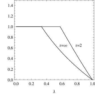
Figure 1: S2S_{2} and S∞S_{\infty}.
rr crc_{r} drd_{r}
2 .577 .732
3 .5 .835
4 .458 .878
10 .381 .953
100 .338 .995
Table 1: Range parameters of Theorem 6.

We are now ready to prove the main theorem.

Theorem 6.
  • (a)

    For all r∈ℕr\in\mathbb{N}, r≥2r\geq 2, and λ∈[0,1]\lambda\in[0,1],

    βrreg​(Δλ)\displaystyle\beta_{r}^{\mathrm{reg}}(\Delta_{\lambda}) =limn→∞1n​βr​(Δλ⊗n)=min⁡{1,2​r−log⁡[(1+3​λ)r+3​(1−λ)r]r−1}\displaystyle=\lim_{n\rightarrow\infty}\,\frac{1}{n}\,\beta_{r}(\Delta_{\lambda}^{\otimes n})=\min\left\{1,\frac{2r-\log\left[(1+3\lambda)^{r}+3(1-\lambda)^{r}\right]}{r-1}\right\} (22)

    in particular

    β2reg​(Δλ)\displaystyle\beta_{2}^{\mathrm{reg}}(\Delta_{\lambda}) ={1λ≤1/32−log⁡(1+3​λ2)λ>1/3,\displaystyle=\begin{cases}1&\lambda\leq 1/\sqrt{3}\\ 2-\log(1+3\lambda^{2})&\lambda>1/\sqrt{3}\end{cases}\,,
    β∞reg​(Δλ)\displaystyle\beta_{\infty}^{\mathrm{reg}}(\Delta_{\lambda}) ={1λ≤1/32−log⁡(1+3​λ)λ>1/3,\displaystyle=\begin{cases}1&\lambda\leq 1/3\\ 2-\log(1+3\lambda)&\lambda>1/3\end{cases}\,,

    where β∞reg​(Δλ)=limr→∞βrreg​(Δλ)\beta_{\infty}^{\mathrm{reg}}(\Delta_{\lambda})=\lim_{r\to\infty}\,\beta_{r}^{\mathrm{reg}}(\Delta_{\lambda}).

  • (b)

    For all r∈ℕr\in\mathbb{N}, r≥2r\geq 2, and λ∈Jr\lambda\in J_{r},

    S¯rreg​(Δλ)=βrreg​(Δλ)\overline{S}_{r}^{\mathrm{reg}}(\Delta_{\lambda})=\beta_{r}^{\mathrm{reg}}(\Delta_{\lambda}) (23)

    where Jr=[0,cr]∪[dr,1]⊂[0,1]J_{r}=[0,c_{r}]\cup[d_{r},1]\subset[0,1] for some 0<cr<dr<10<c_{r}<d_{r}<1 (see Table 1).

The regularized output entropy for r=2r=2 and the lower bound of the same for r=∞r=\infty are plotted in Figure 1. We expect that (23) holds for all λ\lambda. The regularized output entropy is maximal when 2≥(1+3​λ2)r+3​(1−λ2)r2\geq\left(\frac{1+3\lambda}{2}\right)^{r}+3\left(\frac{1-\lambda}{2}\right)^{r} which holds for all rr when λ≤1/3\lambda\leq 1/3. It’s interesting to note that λ≤1/3\lambda\leq 1/3 is also the condition for Δλ\Delta_{\lambda} to be entanglement breaking.

Proof.

(a) From 4.2 we know that 𝒬⁡(id)=2\mathcal{Q}(\mathrm{id})=2 and 𝒬⁡((1​…​r))=(1+3​λ2)r+3​(1−λ2)r\mathcal{Q}((1\dots r))=\left(\frac{1+3\lambda}{2}\right)^{r}+3\left(\frac{1-\lambda}{2}\right)^{r}. In Lemma 13 in 3.1 we prove that one of these two 𝒬\mathcal{Q}-terms yields the maximal value, i.e. for any λ∈[0,1]\lambda\in[0,1]

𝒬max=max⁡{2,(1+3​λ2)r+3​(1−λ2)r}.\mathcal{Q}_{\mathrm{max}}=\max\left\{2,\left(\frac{1+3\lambda}{2}\right)^{r}+3\left(\frac{1-\lambda}{2}\right)^{r}\right\}\,.

Additionally, Δλ\Delta_{\lambda} is entrywise positive for λ∈[0,1]\lambda\in[0,1]. Therefore we can apply parts (a) and (c) of Theorem 4 and (22) follows immediately.

In the case r=2r=2 we have

2⋅2−log⁡[(1+3​λ)2+3​(1−λ)2]2−1\displaystyle\frac{2\cdot 2-\log\left[(1+3\lambda)^{2}+3(1-\lambda)^{2}\right]}{2-1} =4−log⁡(4+12​λ2)\displaystyle=4-\log(4+12\lambda^{2})
=2−log⁡(1+3​λ2),\displaystyle=2-\log(1+3\lambda^{2})\,,

and in the case r=∞r=\infty we have

limr→∞βrreg​(Δλ)\displaystyle\lim_{r\to\infty}\,\beta_{r}^{\mathrm{reg}}(\Delta_{\lambda}) =limr→∞2​r−log⁡[(1+3​λ)r+3​(1−λ)r]r−1\displaystyle=\lim_{r\to\infty}\,\frac{2r-\log\left[(1+3\lambda)^{r}+3(1-\lambda)^{r}\right]}{r-1}
=limr→∞2​r−r​log⁡(1+3​λ)r−1\displaystyle=\lim_{r\to\infty}\,\frac{2r-r\,\log(1+3\lambda)}{r-1}
=2−log⁡(1+3​λ).\displaystyle=2-\log(1+3\lambda)\,.

(b) Define the functions

f⁡(|ϕ⟩)\displaystyle f(|\phi\rangle) =Tr⁡(Δλ⊗n​(|ϕ⟩​⟨ϕ|)r)\displaystyle=\mathrm{Tr}\left(\Delta_{\lambda}^{\otimes n}(|\phi\rangle\langle\phi|)^{r}\right)
g⁡(x)\displaystyle g(x) =1n⁡(1−r)​log⁡x,\displaystyle=\frac{1}{n(1-r)}\log x\,,

and the two series (notice the nn dependency in the definition of ff)

an\displaystyle a_{n} =g⁡(𝔼​f),\displaystyle=g(\mathbb{E}f)\,,
bn\displaystyle b_{n} =𝔼​g∘f.\displaystyle=\mathbb{E}g\circ f\,.

The only difference between ana_{n} and bnb_{n} is the position at which the averaging over pure inputs |ϕ⟩|\phi\rangle takes places. As a result, an=1n​βr​(Δλ⊗n)a_{n}=\frac{1}{n}\beta_{r}(\Delta_{\lambda}^{\otimes n}) contains the average moments that have been considered in previous sections, and bn=1n​Sr​(Δλ⊗n)b_{n}=\frac{1}{n}S_{r}(\Delta_{\lambda}^{\otimes n}) is the Renyi output entropy per systems. By Jensen’s inequality and because the maximal output entropy is log⁡2=1\log 2=1 we have the bounds an≤bn≤1a_{n}\leq b_{n}\leq 1 for any λ\lambda. Our goal is to prove that the two series have the same limit for λ∈[0,cr]∪[dr,1]\lambda\in[0,c_{r}]\cup[d_{r},1].

From part (a) we know

limn→∞an=r−log⁡𝒬maxr−1.\lim_{n\to\infty}a_{n}=\frac{r-\log\mathcal{Q}_{\mathrm{max}}}{r-1}\,.

First, choose c⁡(r)c(r) such that 2≥(1+3​λ2)r+3​(1−λ2)r2\geq\left(\frac{1+3\lambda}{2}\right)^{r}+3\left(\frac{1-\lambda}{2}\right)^{r} for all λ∈[0,c]\lambda\in[0,c]. Then we have 𝒬max=2\mathcal{Q}_{\mathrm{max}}=2, and so

limn→∞an=limn→∞bn=S¯rreg​(Δλ)=1.\lim_{n\to\infty}a_{n}=\lim_{n\to\infty}b_{n}=\overline{S}_{r}^{\mathrm{reg}}(\Delta_{\lambda})=1\,.

Now only (23) remains to be proved for the range λ∈[d,1]\lambda\in[d,1] with dd still to be determined.

In Proposition 18 in 3.2 we prove that the Lipschitz constant η\eta of the map ff is bounded by η≤2​r​κn\eta\leq\sqrt{2}r\kappa^{n} for κ=λ+1−λ2\kappa=\lambda+\frac{1-\lambda}{\sqrt{2}}. From Levy’s Lemma (according to Lemma III.1 in [14]) we know that the values of ff concentrate around their average

Pr⁡(|f⁡(|ϕ⟩)−𝔼​f|>αn)≤4​exp⁡(−C⁡(k+1)​αn2η2)=:ϵn\Pr(|f(|\phi\rangle)-\mathbb{E}f|>\alpha_{n})\leq 4\exp\left(-C(k+1)\frac{\alpha_{n}^{2}}{\eta^{2}}\right)=:\epsilon_{n} (24)

with k=2⋅2n−1k=2\cdot 2^{n}-1 the (real) dimension of the sphere of input states, C=(9​π3​ln⁡2)−1C=(9\pi^{3}\ln 2)^{-1}, and we choose the deviation

αn=12​N​(𝒬max2r)n≈12​𝔼​f\alpha_{n}=\frac{1}{2}N\left(\frac{\mathcal{Q}_{\mathrm{max}}}{2^{r}}\right)^{n}\approx\frac{1}{2}\mathbb{E}f

where N≥1N\geq 1 is the multiplicity of the maximum of 𝒬⁡(α)\mathcal{Q}(\alpha), that is, αn\alpha_{n} is half of the dominant term of 𝔼​f\mathbb{E}f (see prove of Theorem 4). Now αn→0\alpha_{n}\to 0 (apart from the special case λ=1\lambda=1) and 𝔼​f−αn>0\mathbb{E}f-\alpha_{n}>0 which is required in a later step. To ensure concentration for large nn the exponent (k+1)​αn2η2(k+1)\frac{\alpha_{n}^{2}}{\eta^{2}} needs to become large. Taking the 2​n2n-th root we get

((k+1)​αn2η2)1/2​n\displaystyle\left((k+1)\frac{\alpha_{n}^{2}}{\eta^{2}}\right)^{1/2n} =(2⋅22​n​N4​(𝒬max2r)2​n2​r2​κ2​n)1/2​n\displaystyle=\left(2\cdot\sqrt{2}^{2n}\frac{\frac{N}{4}\left(\frac{\mathcal{Q}_{\mathrm{max}}}{2^{r}}\right)^{2n}}{2r^{2}\kappa^{2n}}\right)^{1/2n}
≈2​𝒬max2rκ\displaystyle\approx\sqrt{2}\frac{\frac{\mathcal{Q}_{\mathrm{max}}}{2^{r}}}{\kappa}

where the approximation becomes equality in the large nn limit. If this term is larger than 1 we have the required divergence, this gives the following inequality

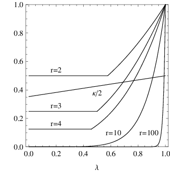
𝒬max2r\displaystyle\frac{\mathcal{Q}_{\mathrm{max}}}{2^{r}} >κ2.\displaystyle>\frac{\kappa}{\sqrt{2}}\,. (25)

This condition gives the lower bound drd_{r} for the λ\lambda values for which (23) holds. Both sides of the inequality are plotted in Figure 2. For some values of rr the range parameters can be found in Table 1.
Refer to caption
Figure 2: Plots of both sides of (25) for some rr values to determine the range of validity.

To transform (24) into a statement about the range of gg – and whence about ana_{n} – we need a condition that implies |f⁡(|ϕ⟩)−𝔼​f|>αn|f(|\phi\rangle)-\mathbb{E}f|>\alpha_{n}. We set αn′=1n⁡(r−1)​αn𝔼​f−αn>|g⁡(𝔼​f)−g⁡(𝔼​f−αn)|>|g⁡(𝔼​f)−g⁡(𝔼​f+αn)|\alpha_{n}^{\prime}=\frac{1}{n(r-1)}\frac{\alpha_{n}}{\mathbb{E}f-\alpha_{n}}>|g(\mathbb{E}f)-g(\mathbb{E}f-\alpha_{n})|>|g(\mathbb{E}f)-g(\mathbb{E}f+\alpha_{n})| where the second inequality follows from convexity of gg. Then for any xx we have

|g⁡(𝔼​f)−g⁡(x)|>αn′⇒|𝔼​f−x|>αn.|g(\mathbb{E}f)-g(x)|>\alpha_{n}^{\prime}\Rightarrow|\mathbb{E}f-x|>\alpha_{n}\,.

Therefore, the values of g∘fg\circ f concentrate around an=g⁡(𝔼​f)a_{n}=g(\mathbb{E}f)

Pr⁡(|g∘f⁡(|ϕ⟩)−an|>αn′)≤ϵn.\Pr(|g\circ f(|\phi\rangle)-a_{n}|>\alpha_{n}^{\prime})\leq\epsilon_{n}\,.

For αn′\alpha_{n}^{\prime} we calculate

limn→∞αn′\displaystyle\lim_{n\to\infty}\alpha_{n}^{\prime} =limn→∞1n⁡(r−1)​αn𝔼​f−αn\displaystyle=\lim_{n\to\infty}\frac{1}{n(r-1)}\frac{\alpha_{n}}{\mathbb{E}f-\alpha_{n}}
=limn→∞1n⁡(r−1)​1/21/2\displaystyle=\lim_{n\to\infty}\frac{1}{n(r-1)}\frac{1/2}{1/2}
=0.\displaystyle=0\,.

To find an upper bound on bnb_{n} assume all |ϕ⟩∈(g∘f)−1​[an−αn′,an+αn′]=B|\phi\rangle\in(g\circ f)^{-1}[a_{n}-\alpha_{n}^{\prime},a_{n}+\alpha_{n}^{\prime}]=B map to the maximal value an+αn′a_{n}+\alpha_{n}^{\prime} and all |ϕ⟩∈Bc|\phi\rangle\in B^{c} map to the maximal value 1. This gives a possible range for the average

bn∈[an,(1−ϵn)​(an+αn′)+ϵn⋅1].b_{n}\in[a_{n},(1-\epsilon_{n})(a_{n}+\alpha_{n}^{\prime})+\epsilon_{n}\cdot 1]\,. (26)

For λ∈[d,1]\lambda\in[d,1] both ϵn\epsilon_{n} and αn′\alpha^{\prime}_{n} tend to 0 for large nn and with (26) and because we know the limit of ana_{n} we have

limn→∞an=limn→∞bn=r−log⁡𝒬maxr−1.\lim_{n\to\infty}a_{n}=\lim_{n\to\infty}b_{n}=\frac{r-\log\mathcal{Q}_{\mathrm{max}}}{r-1}\,.

∎

2.6.3 Output entropy of random sequences

Considering sequences of random pure input states |ϕn⟩|\phi_{n}\rangle with increasing dimension 2n2^{n} we have the following statement.

Proposition 8.

Let |ϕn⟩∈ℂ2n|\phi_{n}\rangle\in\mathbb{C}^{2^{n}} be a sequence of random pure states and

cn=1n​Sr​(Δλ⊗n​(|ϕn⟩​⟨ϕn|))c_{n}=\frac{1}{n}S_{r}(\Delta_{\lambda}^{\otimes n}(|\phi_{n}\rangle\langle\phi_{n}|))

the sequence of output Renyi entropies per system. Then

cn→a.s.r−log⁡𝒬maxr−1c_{n}\stackrel{{\scriptstyle\mathrm{a.s.}}}{{\to}}\frac{r-\log\mathcal{Q}_{\mathrm{max}}}{r-1}

if λ\lambda is restricted as in Theorem 6.

Proof.

Define fn​(|ϕ⟩)=1n​Sr​(Δλ⊗n​(|ϕ⟩​⟨ϕ|))f_{n}(|\phi\rangle)=\frac{1}{n}S_{r}(\Delta_{\lambda}^{\otimes n}(|\phi\rangle\langle\phi|)), the limit value c=r−log⁡𝒬maxr−1=limn→∞𝔼​fnc=\frac{r-\log\mathcal{Q}_{\mathrm{max}}}{r-1}=\lim_{n\to\infty}\mathbb{E}f_{n}, and δn=|𝔼​fn−c|\delta_{n}=|\mathbb{E}f_{n}-c|. Then for any ϵ>0\epsilon>0

Pr⁡(|fn​(|ϕ⟩)−c|>ϵ)\displaystyle\Pr(|f_{n}(|\phi\rangle)-c|>\epsilon) ≤Pr⁡(|fn​(|ϕ⟩)−𝔼​fn|>ϵ−δn)\displaystyle\leq\Pr(|f_{n}(|\phi\rangle)-\mathbb{E}f_{n}|>\epsilon-\delta_{n}) (27)
≤4​exp⁡(−C⁡(k+1)​(ϵ−δn)2η2),\displaystyle\leq 4\exp\left(-C(k+1)\frac{(\epsilon-\delta_{n})^{2}}{\eta^{2}}\right)\,,

with CC, k=2⋅2n−1k=2\cdot 2^{n}-1, and η≤2​r​κn\eta\leq\sqrt{2}r\kappa^{n} with 0<κ<10<\kappa<1 as in the proof of Theorem 6. If λ∈Jr\lambda\in J_{r} then limδn=0\lim\delta_{n}=0. When nn becomes large then kk becomes large, η\eta becomes small, and ϵ−δn\epsilon-\delta_{n} is close to ϵ>0\epsilon>0. Therefore the probabilities in (27) become small. Let NN be such that for n>Nn>N we have δn<ϵ/2\delta_{n}<\epsilon/2. Then we have the bound

∑n=1∞Pr⁡(|fn​(|ϕn⟩)−c|>ϵ)\displaystyle\sum_{n=1}^{\infty}\Pr(|f_{n}(|\phi_{n}\rangle)-c|>\epsilon) ≤∑n=1∞4​exp⁡(−C⁡(k+1)​(ϵ−δn)2η2)\displaystyle\leq\sum_{n=1}^{\infty}4\exp\left(-C(k+1)\frac{(\epsilon-\delta_{n})^{2}}{\eta^{2}}\right)
≤N+∑n>N4​exp⁡(−C⁡(k+1)​(ϵ/2)2η2)\displaystyle\leq N+\sum_{n>N}4\exp\left(-C(k+1)\frac{(\epsilon/2)^{2}}{\eta^{2}}\right)
≤N+∑n>N4​exp⁡(−C~​(2/κ2)n)\displaystyle\leq N+\sum_{n>N}4\exp\left(-\tilde{C}(2/\kappa^{2})^{n}\right)
<∞,\displaystyle<\infty\,,

with C~=C⋅2⋅(ϵ/2)2(2​r)2\tilde{C}=C\cdot 2\cdot\frac{(\epsilon/2)^{2}}{(\sqrt{2}r)^{2}} independent of nn. The Proposition follows by the lemma of Borel-Cantelli. ∎

3 Proof of lemmas

3.1 Maximal 𝒬\mathcal{Q} for Δλ\Delta_{\lambda}

Before proving Proposition 13 which is required for the proof of Theorem 6 we introduce some new notation and we present four lemmas. We only prove our Lemmas in two dimensions, but similar results will hold for higher dimensions.

For the most part we consider a channel 𝒜\mathcal{A} slightly more general than the depolarization channel with

𝒜00=(μ00ν)𝒜11=(ν00μ)𝒜10=(0κλ0)𝒜01=(0λκ0),\begin{array}[]{r@{=}lr@{=}l}\mathcal{A}_{00}&\begin{pmatrix}\mu&0\\ 0&\nu\end{pmatrix}&\mathcal{A}_{11}&\begin{pmatrix}\nu&0\\ 0&\mu\end{pmatrix}\\ \mathcal{A}_{10}&\begin{pmatrix}0&\kappa\\ \lambda&0\end{pmatrix}&\mathcal{A}_{01}&\begin{pmatrix}0&\lambda\\ \kappa&0\end{pmatrix}\end{array}\,,

where κ,λ,μ,ν∈ℝ0+\kappa,\lambda,\mu,\nu\in\mathbb{R}_{0}^{+} and μ≥ν\mu\geq\nu, λ≥κ\lambda\geq\kappa. We call this channel the two-rail channel. Remember that in the case 𝒜=Δλ\mathcal{A}=\Delta_{\lambda} we have μ=1+λ2\mu=\frac{1+\lambda}{2}, ν=1−λ2\nu=\frac{1-\lambda}{2} and κ=0\kappa=0. Because all these matrix entries are positive, so are the 𝒬\mathcal{Q}-terms, and therefore the largest positive 𝒬\mathcal{Q}-term will yield 𝒬max\mathcal{Q}_{\mathrm{max}}.

We think of these matrices as the diagrams in Figure 4. We refer to the lines as rails and to their vertical position as their track (starting with track 0)

Refer to caption
Figure 3: The diagrams for the 𝒜x​y\mathcal{A}_{xy} matrices.
𝒜00​𝒜01​𝒜10​𝒜11​𝒜10\mathcal{A}_{00}\mathcal{A}_{01}\mathcal{A}_{10}\mathcal{A}_{11}\mathcal{A}_{10}
Refer to caption
Figure 4: A product of 𝒜x​y\mathcal{A}_{xy} matrices and the corresponding diagram.

A product looks like the diagram in Figure 4, notice that we read from right to left, the same way that matrix multiplication applies. Consider a vector multiplying with this product, the diagram can be thought of as presenting two rails along which the two entries of the vector pass through to the left. On the way, continuous lines multiply the entries with factors μ\mu or λ\lambda, dashed lines with a factor ν\nu or κ\kappa. Because the products are inside a trace, they will only contribute, if the rail starting at the top on the right, ends on the top at the left (giving the ⟨0|…|0⟩\langle 0|\dots|0\rangle contribution), and the same for the rail starting at the bottom (giving the ⟨1|…|1⟩\langle 1|\dots|1\rangle contribution). Using this, we can compare contributions to 𝒬⁡(α)\mathcal{Q}(\alpha) for different α\alpha.

We rewrite

𝒬⁡(α)=∑δ∈𝒟⁡(α)Tr⁡(δ)\mathcal{Q}(\alpha)=\sum_{\delta\in\mathcal{D}(\alpha)}\mathrm{Tr}\left(\delta\right)

where 𝒟⁡(α)\mathcal{D}(\alpha) is the set of 2r2^{r} diagrams corresponding to α\alpha and we identify the diagram δ\delta with the corresponding matrix.

Furthermore, for a diagram δ\delta we define δ1\delta^{1} to be the unchanged diagram and δ−1\delta^{-1} to be the horizontally reflected diagram. If we take 𝒟0​(α)\mathcal{D}_{0}(\alpha) to be the set of all diagrams in 𝒟⁡(α)\mathcal{D}(\alpha) that start high (at track 0) then obviously 𝒟⁡(α)=𝒟0​(α)∪𝒟0−1​(α)\mathcal{D}(\alpha)=\mathcal{D}_{0}(\alpha)\cup\mathcal{D}_{0}^{-1}(\alpha) provides a convenient splitting of the sum in 𝒬⁡(α)\mathcal{Q}(\alpha).

We say an α\alpha is non-overlapping if all its cycles permute consecutive numbers, e.g. α=(123)​(45)​(678)\alpha=(123)(45)(678). For such α\alpha we write α=α1​…​αs\alpha=\alpha_{1}\dots\alpha_{s}, where all the αi\alpha_{i} are the cycles. We define a product for diagrams by simply concatenating them. With this product we get 𝒟⁡(α)=𝒟⁡(α1)​…​𝒟​(αs)\mathcal{D}(\alpha)=\mathcal{D}(\alpha_{1})\dots\mathcal{D}(\alpha_{s}).

Lemma 9.

Consider a diagram δ∈𝒟⁡((1​…​r))\delta\in\mathcal{D}((1\dots r)) of a two-rail channel. Then we have

δ+δ−1∝𝟙.\delta+\delta^{-1}\propto\mathbbm{1}\,.
Proof.

In any diagram δ∈𝒟⁡((1​…​r))\delta\in\mathcal{D}((1\dots r)) one rail starts and ends at track 0 and the other starts and ends at track 1. That means the corresponding matrix is diagonal. Reflecting the diagram simply means exchanging the two diagonal entries, and if we sum δ+δ−1\delta+\delta^{-1} then the diagonal entries both have the same sum, i.e. it is proportional to unity.∎

Lemma 10.

Let α=α1​…​αs∈S​y​m​(r)\alpha=\alpha_{1}\dots\alpha_{s}\in Sym(r) be a non-overlapping permutation consisting of ss cycles. Then the 𝒬⁡(α)\mathcal{Q}(\alpha) of a two-rail channel factors like

𝒬⁡(α)=12s−1​𝒬​(α1)​…​𝒬​(αs).\mathcal{Q}(\alpha)=\frac{1}{2^{s-1}}\mathcal{Q}(\alpha_{1})\dots\mathcal{Q}(\alpha_{s})\,.
Proof.

First we use the fact, that the diagrams for a non-overlapping α\alpha can be split between cycles, i.e. the sum splits into sums over separate diagrams,

𝒬⁡(α)\displaystyle\mathcal{Q}(\alpha) =∑δ∈𝒟⁡(α)Tr⁡(δ)\displaystyle=\sum_{\delta\in\mathcal{D}(\alpha)}\mathrm{Tr}\left(\delta\right)
=∑δ1∈𝒟⁡(α1)…​∑δs∈𝒟⁡(αs)Tr⁡(δ1​…​δs)\displaystyle=\sum_{\delta_{1}\in\mathcal{D}(\alpha_{1})}\dots\sum_{\delta_{s}\in\mathcal{D}(\alpha_{s})}\mathrm{Tr}\left(\delta_{1}\dots\delta_{s}\right)
=Tr⁡(∑δ1∈𝒟⁡(α1)δ1​…​∑δs∈𝒟⁡(αs)δs).\displaystyle=\mathrm{Tr}\left(\sum_{\delta_{1}\in\mathcal{D}(\alpha_{1})}\delta_{1}\dots\sum_{\delta_{s}\in\mathcal{D}(\alpha_{s})}\delta_{s}\right)\,.

Using the splitting 𝒟⁡(α)=𝒟0​(α)∪𝒟0−1​(α)\mathcal{D}(\alpha)=\mathcal{D}_{0}(\alpha)\cup\mathcal{D}_{0}^{-1}(\alpha) and Lemma 9 we have

∑δ∈𝒟⁡(αi)δ=∑δ∈𝒟0​(αi)δ+δ−1∝𝟙\sum_{\delta\in\mathcal{D}(\alpha_{i})}\delta=\sum_{\delta\in\mathcal{D}_{0}(\alpha_{i})}\delta+\delta^{-1}\propto\mathbbm{1}

for all ss cycles αi\alpha_{i}. Therefore, we can split the single trace into ss separate traces

𝒬⁡(α)\displaystyle\mathcal{Q}(\alpha) =12s−1​∑δ1∈𝒟⁡(α1)Tr⁡(δ1)​…​∑δ1∈𝒟⁡(αs)Tr⁡(δs)\displaystyle=\frac{1}{2^{s-1}}\sum_{\delta_{1}\in\mathcal{D}(\alpha_{1})}\mathrm{Tr}\left(\delta_{1}\right)\dots\sum_{\delta_{1}\in\mathcal{D}(\alpha_{s})}\mathrm{Tr}\left(\delta_{s}\right)
=12s−1​𝒬​(α1)​…​𝒬​(αs).\displaystyle=\frac{1}{2^{s-1}}\mathcal{Q}(\alpha_{1})\dots\mathcal{Q}(\alpha_{s})\,.

∎

Lemma 11.

For 𝒜=Δλ\mathcal{A}=\Delta_{\lambda} the depolarizing channel in two dimensions, 𝒬\mathcal{Q} restricted to non-overlapping permutations α∈S​y​m​(r)\alpha\in Sym(r) is either maximal when α=(1​…​r)\alpha=(1\dots r) or when α=id\alpha=\mathrm{id}.

Proof.

Remember from 2.6.1 that 𝒬⁡((1​…​r))=(μ+λ)r+3​νr\mathcal{Q}((1\dots r))=(\mu+\lambda)^{r}+3\nu^{r}. It is convenient to introduce

f⁡(x)=(μ+λ)x+3​νx,f(x)=(\mu+\lambda)^{x}+3\nu^{x}\,,

as a function with range ℝ\mathbb{R}. For a pure α=α1​…​αs\alpha=\alpha_{1}\dots\alpha_{s} according to Lemma 10 we get

𝒬⁡(α)=12s−1​∏i=1sf⁡(|αi|).\mathcal{Q}(\alpha)=\frac{1}{2^{s-1}}\prod_{i=1}^{s}f(|\alpha_{i}|)\,. (28)

with |αi||\alpha_{i}| denoting the length of a cycle.

In the following we keep the number ss of cycles and the total length rr of the permutation invariant. Now, if we increase the length of one cycle and decrease the length of another, we are only changing two factors in the product, f⁡(x)​f​(k−x)f(x)f(k-x), where xx is the length of the first cycle and kk the (invariant) sum of the lengths of both cycles. We rewrite

f⁡(x)​f​(k−x)\displaystyle f(x)f(k-x) =((μ+λ)x+3​νx)​((μ+λ)k−x+3​νk−x)\displaystyle=((\mu+\lambda)^{x}+3\nu^{x})((\mu+\lambda)^{k-x}+3\nu^{k-x})
=(μ+λ)k+9​νk+3​νk​(μ+λν)x+3​(μ+λ)k​(νμ+λ)x.\displaystyle=(\mu+\lambda)^{k}+9\nu^{k}+3\nu^{k}\left(\frac{\mu+\lambda}{\nu}\right)^{x}+3(\mu+\lambda)^{k}\left(\frac{\nu}{\mu+\lambda}\right)^{x}\,.

Because of μ+λ,ν≥0\mu+\lambda,\nu\geq 0 the function f⁡(x)​f​(k−x)f(x)f(k-x) is convex in xx. Therefore it is maximal at the boundaries, i.e. when one cycle has the minimal length of 1. If we repeat this procedure s−1s-1 times we end up with one large cycle of length t=r−s+1t=r-s+1 while all other cycles are of length 1. In every step we increase 𝒬\mathcal{Q}, so we get the bound

𝒬⁡(α)≤𝒬⁡((1)​(2)​…​(s−1)​(s​…​r))=12s−1​f​(1)s−1​f​(t)=f⁡(t)\mathcal{Q}(\alpha)\leq\mathcal{Q}((1)(2)\dots(s-1)(s\dots r))=\frac{1}{2^{s-1}}f(1)^{s-1}f(t)=f(t) (29)

for non-overlapping permutations α\alpha consisting of ss cycles.

Now compare the upper bounds given by (29) for permutations of the same total length rr but different number of cycles ss. This is the same as varying tt . Because ff is convex we get a maximal upper bound if tt is minimal or maximal. The minimal value t=1t=1 is achieved when s=rs=r and all the cycles are of length 1. Then (29) becomes an equality - there are no steps necessary in the maximization procedure - and we have 𝒬⁡(id)=f⁡(1)=2\mathcal{Q}(\mathrm{id})=f(1)=2. The maximal value t=rt=r is achieved when α\alpha is simply one large cycle. Again (29) becomes equality, and 𝒬⁡(α)=f⁡(r)\mathcal{Q}(\alpha)=f(r). One of these upper bounds is the highest upper bound possible in (29), and because they are achieved by 𝒬⁡(id)\mathcal{Q}(\mathrm{id}) and 𝒬⁡((1​…​r))\mathcal{Q}((1\dots r)) we know that one of these 𝒬⁡(α)\mathcal{Q}(\alpha) is maximal over α∈S​y​m​(r)\alpha\in Sym(r).∎

Lemma 12.

Let 𝒜\mathcal{A} be a two-rail channel, and [β][\beta] the conjugacy class of a permutation. Then 𝒬\mathcal{Q} restricted to [β][\beta] is maximal on non-overlapping members α∈[β]\alpha\in[\beta].

Proof.

Let α=α1​…​αs\alpha=\alpha_{1}\dots\alpha_{s} be a non-overlapping member of the class and β=γ​α​γ−1\beta=\gamma\alpha\gamma^{-1} be any other member of the class. First, remember

𝒬⁡(α)=∑{xi}i=1​…​rTr⁡(∏i=1r𝒜xi​xα⁡(i))=∑δ1∈𝒟⁡(α1)…​∑δs∈𝒟⁡(αs)Tr⁡(δ1​…​δs).\mathcal{Q}(\alpha)=\sum_{\begin{subarray}{c}\{x_{i}\}\\ i=1\dots r\end{subarray}}\mathrm{Tr}\left(\prod_{i=1}^{r}\mathcal{A}_{x_{i}x_{\alpha(i)}}\right)=\sum_{\delta_{1}\in\mathcal{D}(\alpha_{1})}\dots\sum_{\delta_{s}\in\mathcal{D}(\alpha_{s})}\mathrm{Tr}\left(\delta_{1}\dots\delta_{s}\right)\,. (30)

With the first way of writing 𝒬⁡(α)\mathcal{Q}(\alpha) in mind we define a 1-1-mapping between terms in the sum of 𝒬⁡(α)\mathcal{Q}(\alpha) and 𝒬⁡(β)\mathcal{Q}(\beta) via a mapping of indices xi→xγ−1​(i)x_{i}\to x_{\gamma^{-1}(i)} (or xγ⁡(i)→xix_{\gamma(i)}\to x_{i}). Then the products of matrices are mapped like

𝒜x1​xα⁡(1)​…​𝒜xr​xα⁡(r)\displaystyle\mathcal{A}_{x_{1}x_{\alpha(1)}}\dots\mathcal{A}_{x_{r}x_{\alpha(r)}} →𝒜xγ⁡(1)​xγ⁡(β⁡(1))​…​𝒜xγ⁡(r)​xγ⁡(β⁡(r))\displaystyle\to\mathcal{A}_{x_{\gamma(1)}x_{\gamma(\beta(1))}}\dots\mathcal{A}_{x_{\gamma(r)}x_{\gamma(\beta(r))}}
=𝒜xγ⁡(1)​xα⁡(γ⁡(1))​…​𝒜xγ⁡(r)​xα⁡(γ⁡(r)).\displaystyle=\mathcal{A}_{x_{\gamma(1)}x_{\alpha(\gamma(1))}}\dots\mathcal{A}_{x_{\gamma(r)}x_{\alpha(\gamma(r))}}\,.

In terms of diagrams this corresponds to permuting the “tiles” (crossings or straight pieces) 𝒜xi​xα⁡(i)\mathcal{A}_{x_{i}x_{\alpha(i)}} according to the permutation γ\gamma. Some examples are shown in Appendix A. In particular, this mapping does not change the number of any kind of tile 𝒜00\mathcal{A}_{00}, 𝒜01\mathcal{A}_{01}, 𝒜10\mathcal{A}_{10} or 𝒜11\mathcal{A}_{11}.

Now, consider the second way of writing 𝒬⁡(α)\mathcal{Q}(\alpha) in (30) and split the sums over subdiagrams 𝒟⁡(αi)\mathcal{D}(\alpha_{i}) according to 𝒟⁡(αi)=𝒟0​(αi)∪𝒟0−1​(αi)\mathcal{D}(\alpha_{i})=\mathcal{D}_{0}(\alpha_{i})\cup\mathcal{D}_{0}^{-1}(\alpha_{i})

𝒬⁡(α)=∑δ1∈𝒟0​(α1)…​∑δs∈𝒟0​(αs)∑{ti=±1}i=1​…​sTr⁡(δ1t1​…​δsts).\mathcal{Q}(\alpha)=\sum_{\delta_{1}\in\mathcal{D}_{0}(\alpha_{1})}\dots\sum_{\delta_{s}\in\mathcal{D}_{0}(\alpha_{s})}\sum_{\begin{subarray}{c}\{t_{i}=\pm 1\}\\ i=1\dots s\end{subarray}}\mathrm{Tr}\left(\delta_{1}^{t_{1}}\dots\delta_{s}^{t_{s}}\right)\,.

We consider a subsum

∑{ti=±1}i=1​…​sTr⁡(δ1t1​…​δsts)\sum_{\begin{subarray}{c}\{t_{i}=\pm 1\}\\ i=1\dots s\end{subarray}}\mathrm{Tr}\left(\delta_{1}^{t_{1}}\dots\delta_{s}^{t_{s}}\right)

for fixed subdiagrams δi∈𝒟0​(αi)\delta_{i}\in\mathcal{D}_{0}(\alpha_{i}). In the following we will prove that the contribution of this subsum to 𝒬⁡(α)\mathcal{Q}(\alpha) is larger or equal to the contribution of the subsum of the corresponding diagrams to 𝒬⁡(β)\mathcal{Q}(\beta). From this it immediately follows that 𝒬⁡(α)≥𝒬⁡(β)\mathcal{Q}(\alpha)\geq\mathcal{Q}(\beta).

It follows a general proof of the inequality between corresponding subsums. For illustration one subsum is evaluated in full detail with diagrams in Appendix A.

For the non-overlapping permutation α\alpha in the subdiagrams δi\delta_{i} all the straight lines and dashed lines are aligned, i.e. we have a weak and a strong rail. Let mim_{i} be the number of crossings and nin_{i} the number of straight pieces in δi\delta_{i}. The strong rail in subdiagram δi\delta_{i} contributes a factor λmi​μni\lambda^{m_{i}}\mu^{n_{i}} and the weak rail contributes the factor κmi​νni\kappa^{m_{i}}\nu^{n_{i}}. Summing over reflections the subsum equals

2​∏i=1sλmi​μni+κmi​νni.2\prod_{i=1}^{s}\lambda^{m_{i}}\mu^{n_{i}}+\kappa^{m_{i}}\nu^{n_{i}}\,.

On the other hand, for the possibly overlapping β\beta some of the tiles are permuted and for one particular subdiagram, not all the strong rail pieces might be on the same rail. Let m~i\tilde{m}_{i} be the number of crossings that are thus misaligned and n~i\tilde{n}_{i} the number of straight pieces that are misaligned. The two rails in subdiagram δi\delta_{i} now contribute the factors λmi−m~i​κm~i​μni−n~i​νn~i\lambda^{m_{i}-\tilde{m}_{i}}\kappa^{\tilde{m}_{i}}\mu^{n_{i}-\tilde{n}_{i}}\nu^{\tilde{n}_{i}} and λm~i​κmi−m~i​μn~i​νni−n~i\lambda^{\tilde{m}_{i}}\kappa^{m_{i}-\tilde{m}_{i}}\mu^{\tilde{n}_{i}}\nu^{n_{i}-\tilde{n}_{i}}. Summing over reflections the subsum adding to 𝒬⁡(β)\mathcal{Q}(\beta) equals

2​∏i=1sλmi−m~i​κm~i​μni−n~i​νn~i+λm~i​κmi−m~i​μn~i​νni−n~i.2\prod_{i=1}^{s}\lambda^{m_{i}-\tilde{m}_{i}}\kappa^{\tilde{m}_{i}}\mu^{n_{i}-\tilde{n}_{i}}\nu^{\tilde{n}_{i}}+\lambda^{\tilde{m}_{i}}\kappa^{m_{i}-\tilde{m}_{i}}\mu^{\tilde{n}_{i}}\nu^{n_{i}-\tilde{n}_{i}}\,.

Because λ≥κ\lambda\geq\kappa and μ≥ν\mu\geq\nu it follows that λmi​μni+κmi​νni≥λmi−m~i​κm~i​μni−n~i​νn~i+λm~i​κmi−m~i​μn~i​νni−n~i\lambda^{m_{i}}\mu^{n_{i}}+\kappa^{m_{i}}\nu^{n_{i}}\geq\lambda^{m_{i}-\tilde{m}_{i}}\kappa^{\tilde{m}_{i}}\mu^{n_{i}-\tilde{n}_{i}}\nu^{\tilde{n}_{i}}+\lambda^{\tilde{m}_{i}}\kappa^{m_{i}-\tilde{m}_{i}}\mu^{\tilde{n}_{i}}\nu^{n_{i}-\tilde{n}_{i}} (the strong and weak rail dominate the two mixed rails), and hence we have the desired inequality between corresponding contributions to 𝒬⁡(α)\mathcal{Q}(\alpha) and 𝒬⁡(β)\mathcal{Q}(\beta).∎

Proposition 13.

For 𝒜=Δλ\mathcal{A}=\Delta_{\lambda} the depolarizing channel in two dimensions, 𝒬⁡(α)\mathcal{Q}(\alpha) is either maximal when α=(1​…​r)\alpha=(1\dots r) or when α=id\alpha=\mathrm{id}.

Proof.

First, consider permutations that consist of non-overlapping α\alpha, Lemma 11 proves that either α=id\alpha=\mathrm{id} or α=(1​…​r)\alpha=(1\dots r) yields the maximum 𝒬⁡(α)\mathcal{Q}(\alpha) amongst these permutations. Every conjugacy class has a non-overlapping representant, and Lemma 12 states that these have maximal 𝒬\mathcal{Q}-value. Therefore either α=id\alpha=\mathrm{id} or α=(1​…​r)\alpha=(1\dots r) yield the maximal 𝒬\mathcal{Q}-value amongst all the permutations α∈S​y​m​m​(r)\alpha\in Symm(r). ∎

3.2 Bound on Lipschitz constant

We derive an upper bound on the Lipschitz constant of the function f:S2n+1−1→ℝf:S^{2^{n+1}-1}\to\mathbb{R}

f⁡(|ϕ⟩)=Tr⁡(Δλ⊗n​(|ϕ⟩​⟨ϕ|)r)f(|\phi\rangle)=\mathrm{Tr}\left(\Delta_{\lambda}^{\otimes n}(|\phi\rangle\langle\phi|)^{r}\right)

with respect to the Euclidean norm on S2n+1−1⊂ℝ2n+1S^{2^{n+1}-1}\subset\mathbb{R}^{2^{n+1}}.

We divide the function into four steps and prove bounds on the Lipschitz constants for each step. The splitting is f=d∘c∘b∘af=d\circ c\circ b\circ a with

a\displaystyle a :|ϕ⟩→|ϕ⟩​⟨ϕ|=ρ\displaystyle:|\phi\rangle\to|\phi\rangle\langle\phi|=\rho
b\displaystyle b :ρ→Δλ⊗n​(ρ)=ρ′\displaystyle:\rho\rightarrow\Delta_{\lambda}^{\otimes n}(\rho)=\rho^{\prime}
c\displaystyle c :ρ′→eigenvalues of ​ρ′=v→\displaystyle:\rho^{\prime}\rightarrow\textrm{eigenvalues of }\rho^{\prime}=\vec{v}
d\displaystyle d :v→→∑ivir.\displaystyle:\vec{v}\rightarrow\sum_{i}v_{i}^{r}\,.

Let ℳm\mathcal{M}_{m} be the space of complex m×mm\times m matrices containing the set of states 𝒮m={ρ∈ℳm:ρ=ρ∗,Trρ=1}\mathcal{S}_{m}=\{\rho\in\mathcal{M}_{m}:\rho=\rho^{*},\mathrm{Tr\,}\rho=1\}.

Lemma 14.

Let a⁡(|ϕ⟩)=|ϕ⟩​⟨ϕ|a(|\phi\rangle)=|\phi\rangle\langle\phi| a map ℂm→ℳm\mathbb{C}^{m}\to\mathcal{M}_{m} where ⟨ϕ|ϕ⟩=1\left\langle\phi\middle|\phi\right\rangle=1. Then the Lipschitz constant of aa with respect to the Euclidean norm in the domain and the Frobenius norm ‖M‖2=Tr​(M​M∗)1/2\|M\|_{2}=\mathrm{Tr}\left(MM^{*}\right)^{1/2} in the range is upper bounded by 2\sqrt{2}.

Proof.

For ⟨ϕ|ϕ⟩=⟨ψ|ψ⟩=1\left\langle\phi\middle|\phi\right\rangle=\left\langle\psi\middle|\psi\right\rangle=1 set c=⟨ϕ|ψ⟩c=\left\langle\phi\middle|\psi\right\rangle. Now

‖|ϕ⟩−|ψ⟩‖22=⟨ϕ|ϕ⟩−⟨ϕ|ψ⟩−⟨ψ|ϕ⟩+⟨ψ|ψ⟩=2−2​ℜ⁡(c),\||\phi\rangle-|\psi\rangle\|_{2}^{2}=\left\langle\phi\middle|\phi\right\rangle-\left\langle\phi\middle|\psi\right\rangle-\left\langle\psi\middle|\phi\right\rangle+\left\langle\psi\middle|\psi\right\rangle=2-2\Re(c)\,,

and

‖|ϕ⟩​⟨ϕ|−|ψ⟩​⟨ψ|‖22=⟨ϕ|ϕ⟩2−2​|⟨ϕ|ψ⟩|2+⟨ψ|ψ⟩2=2−2​|c|2.\||\phi\rangle\langle\phi|-|\psi\rangle\langle\psi|\|_{2}^{2}=\left\langle\phi\middle|\phi\right\rangle^{2}-2|\left\langle\phi\middle|\psi\right\rangle|^{2}+\left\langle\psi\middle|\psi\right\rangle^{2}=2-2|c|^{2}\,.

Because of ℜ⁡(c)≤|c|\Re(c)\leq|c| and the inequality derived as follows

(1−|c|)2\displaystyle(1-|c|)^{2} ≥0\displaystyle\geq 0
2−2​|c|\displaystyle 2-2|c| ≥1−|c|2\displaystyle\geq 1-|c|^{2}
2​(2−2​|c|)\displaystyle 2(2-2|c|) ≥2−2​|c|2,\displaystyle\geq 2-2|c|^{2}\,,

we arrive at 2​(2−2​ℜ⁡(c))≥2−2​|c|22(2-2\Re(c))\geq 2-2|c|^{2} or 2​‖|ϕ⟩−|ψ⟩‖2≥‖|ϕ⟩​⟨ϕ|−|ψ⟩​⟨ψ|‖2\sqrt{2}\||\phi\rangle-|\psi\rangle\|_{2}\geq\||\phi\rangle\langle\phi|-|\psi\rangle\langle\psi|\|_{2}.∎

Lemma 15.

Let b⁡(ρ)=Δλ⊗n​(ρ)b(\rho)=\Delta_{\lambda}^{\otimes n}(\rho) a map 𝒮2n→𝒮2n\mathcal{S}_{2^{n}}\to\mathcal{S}_{2^{n}}, then the Lipschitz constant of bb with respect to the Frobenius norm in domain and range is upper bounded by κn\kappa^{n}, where κ=λ+1−λ2\kappa=\lambda+\frac{1-\lambda}{\sqrt{2}} so 0<κ<10<\kappa<1 for 0<λ<10<\lambda<1.

Proof.

It is useful to use the notation

Δλ⊗n=∑J⊂ℤnλn−|J|​(1−λ)|J|​TrJ⊗(𝟙2)⊗|J|\Delta_{\lambda}^{\otimes n}=\sum_{J\subset\mathbb{Z}_{n}}\lambda^{n-|J|}(1-\lambda)^{|J|}\mathrm{Tr\,}_{J}\otimes\left(\frac{\mathbbm{1}}{2}\right)^{\otimes|J|}

where TrJ\mathrm{Tr\,}_{J} is the partial trace over the systems with indices in JJ. Notice that we use a loose notation of the tensor product as the systems that are partially traced out and replaced by the totally mixed states are not necessarily all on the right side of the tensor product.

We will bound the operator norm ‖𝒜‖o​p:=supρ∈S‖𝒜⁡(ρ)‖2‖ρ‖2\|\mathcal{A}\|_{op}:=\sup_{\rho\in S}\frac{\|\mathcal{A}(\rho)\|_{2}}{\|\rho\|_{2}} where the supremum is over the set S={|ϕ⟩⟨ϕ|−|ψ⟩⟨ψ|||ϕ⟩,|ψ⟩∈𝒮2n−1}S=\left\{|\phi\rangle\langle\phi|-|\psi\rangle\langle\psi|\,\middle|\,|\phi\rangle,|\psi\rangle\in\mathcal{S}_{2^{n}-1}\right\}. Because of

‖𝒜⁡(ρ)−𝒜⁡(τ)‖2=‖𝒜⁡(ρ−τ)‖2≤‖𝒜‖o​p​‖ρ−τ‖2\|\mathcal{A}(\rho)-\mathcal{A}(\tau)\|_{2}=\|\mathcal{A}(\rho-\tau)\|_{2}\leq\|\mathcal{A}\|_{op}\|\rho-\tau\|_{2}

for a linear map 𝒜\mathcal{A} bounding ‖𝒜‖o​p\|\mathcal{A}\|_{op} immediately gives a bound of the Lipschitz constant as well. Now

‖Δλ⊗n‖o​p\displaystyle\|\Delta_{\lambda}^{\otimes n}\|_{op} ≤∑Jλn−|J|​(1−λ)|J|​‖TrJ⊗(𝟙2)⊗|J|‖o​p\displaystyle\leq\sum_{J}\lambda^{n-|J|}(1-\lambda)^{|J|}\left\|\mathrm{Tr\,}_{J}\otimes\left(\frac{\mathbbm{1}}{2}\right)^{\otimes|J|}\right\|_{op}
≤∑Jλn−|J|​(1−λ2)|J|\displaystyle\leq\sum_{J}\lambda^{n-|J|}\left(\frac{1-\lambda}{\sqrt{2}}\right)^{|J|}
=∑k=0n(nk)​λn−k​(1−λ2)k\displaystyle=\sum_{k=0}^{n}{n\choose k}\lambda^{n-k}\left(\frac{1-\lambda}{\sqrt{2}}\right)^{k}
=(λ+1−λ2)n=κn,\displaystyle=\left(\lambda+\frac{1-\lambda}{\sqrt{2}}\right)^{n}=\kappa^{n}\,,

where we used the bound

‖Tr{1​…​k}⊗(𝟙2)⊗k‖o​p2\displaystyle\left\|\mathrm{Tr\,}_{\{1\dots k\}}\otimes\left(\frac{\mathbbm{1}}{2}\right)^{\otimes k}\right\|_{op}^{2} =supρ∈STr​(Tr{1​…​k}​ρ⊗(𝟙2)⊗k)2Tr​ρ2\displaystyle=\sup_{\rho\in S}\frac{\mathrm{Tr\,}\left(\mathrm{Tr\,}_{\{1\dots k\}}\rho\otimes\left(\frac{\mathbbm{1}}{2}\right)^{\otimes k}\right)^{2}}{\mathrm{Tr\,}\rho^{2}}
=Tr​((𝟙2)⊗k)2​supρ∈STr​(Tr{1​…​k}​ρ)2Tr​ρ2\displaystyle=\mathrm{Tr\,}\left(\left(\frac{\mathbbm{1}}{2}\right)^{\otimes k}\right)^{2}\sup_{\rho\in S}\frac{\mathrm{Tr\,}\left(\mathrm{Tr\,}_{\{1\dots k\}}\rho\right)^{2}}{\mathrm{Tr\,}\rho^{2}} (31)
=(12)k.\displaystyle=\left(\frac{1}{2}\right)^{k}\,.

The supremum in (31) was evaluated as follows. First, consider that ρ=|ϕ⟩​⟨ϕ|−|ψ⟩​⟨ψ|\rho=|\phi\rangle\langle\phi|-|\psi\rangle\langle\psi| can be written as ρ=α⁡|0⟩​⟨0|−α|1⟩​⟨1|\rho=\alpha|0\rangle\langle 0|-\alpha|1\rangle\langle 1| with 0≤α≤10\leq\alpha\leq 1, where |0⟩|0\rangle and |1⟩|1\rangle are orthonormal states. Then the supremum runs over all possible orientations of |0⟩|0\rangle and |1⟩|1\rangle

supρ∈STr​(Tr{1​…​k}​ρ)2Tr​ρ2\displaystyle\sup_{\rho\in S}\frac{\mathrm{Tr\,}\left(\mathrm{Tr\,}_{\{1\dots k\}}\rho\right)^{2}}{\mathrm{Tr\,}\rho^{2}} =sup|0⟩,|1⟩Tr​(Tr{1​…​k}​(α⁡|0⟩​⟨0|−α|1⟩​⟨1|))2Tr​(α⁡|0⟩​⟨0|−α|1⟩​⟨1|)2\displaystyle=\sup_{|0\rangle,|1\rangle}\frac{\mathrm{Tr\,}\left(\mathrm{Tr\,}_{\{1\dots k\}}(\alpha|0\rangle\langle 0|-\alpha|1\rangle\langle 1|)\right)^{2}}{\mathrm{Tr\,}(\alpha|0\rangle\langle 0|-\alpha|1\rangle\langle 1|)^{2}}
=sup|0⟩,|1⟩Tr​(Tr{1​…​k}​(|0⟩​⟨0|−|1⟩​⟨1|))2Tr​(|0⟩​⟨0|−|1⟩​⟨1|)2\displaystyle=\sup_{|0\rangle,|1\rangle}\frac{\mathrm{Tr\,}\left(\mathrm{Tr\,}_{\{1\dots k\}}(|0\rangle\langle 0|-|1\rangle\langle 1|)\right)^{2}}{\mathrm{Tr\,}(|0\rangle\langle 0|-|1\rangle\langle 1|)^{2}}
=sup|0⟩,|1⟩Tr​(Tr{1​…​k}​(|0⟩​⟨0|−|1⟩​⟨1|))22.\displaystyle=\sup_{|0\rangle,|1\rangle}\frac{\mathrm{Tr\,}\left(\mathrm{Tr\,}_{\{1\dots k\}}(|0\rangle\langle 0|-|1\rangle\langle 1|)\right)^{2}}{2}\,.

Now assume ρ0=Tr{1​…​k}​|0⟩​⟨0|\rho_{0}=\mathrm{Tr\,}_{\{1\dots k\}}|0\rangle\langle 0| and ρ1=Tr{1​…​k}​|1⟩​⟨1|\rho_{1}=\mathrm{Tr\,}_{\{1\dots k\}}|1\rangle\langle 1| are arbitrary density matrices. Then

sup|0⟩,|1⟩Tr​(Tr{1​…​k}​(|0⟩​⟨0|−|1⟩​⟨1|))22\displaystyle\sup_{|0\rangle,|1\rangle}\frac{\mathrm{Tr\,}\left(\mathrm{Tr\,}_{\{1\dots k\}}(|0\rangle\langle 0|-|1\rangle\langle 1|)\right)^{2}}{2} =supρ0,ρ1Tr​(ρ0−ρ1)22\displaystyle=\sup_{\rho_{0},\rho_{1}}\frac{\mathrm{Tr}\left(\rho_{0}-\rho_{1}\right)^{2}}{2}
=supρ0,ρ1Tr⁡(ρ02+ρ12−2​ρ0​ρ1)2=1.\displaystyle=\sup_{\rho_{0},\rho_{1}}\frac{\mathrm{Tr}\left(\rho_{0}^{2}+\rho_{1}^{2}-2\rho_{0}\rho_{1}\right)}{2}=1\,.

The last equality follows from the fact, that Tr​ρ0,12≤1\mathrm{Tr\,}\rho_{0,1}^{2}\leq 1 and Tr​ρ0​ρ1≥0\mathrm{Tr\,}\rho_{0}\rho_{1}\geq 0. The suprema are achieved when |ϕ⟩=|00⟩|\phi\rangle=|00\rangle and |ψ⟩=|11⟩|\psi\rangle=|11\rangle so that ρ0=|0⟩​⟨0|\rho_{0}=|0\rangle\langle 0| and ρ1=|1⟩​⟨1|\rho_{1}=|1\rangle\langle 1|.∎

Remark 16.

Let c:𝒮m→ℝmc:\mathcal{S}_{m}\rightarrow\mathbb{R}^{m} be the map that sends density matrices to their eigenvalues, ordered high to low. The fact that the Lipschitz constant of cc is upper bounded by 11 is equivalent to the Hoffman-Wielandt inequality [19]

‖ρ−τ‖2≥‖c⁡(ρ)−c⁡(τ)‖2.\|\rho-\tau\|_{2}\geq\|c(\rho)-c(\tau)\|_{2}\,.
Lemma 17.

Let d⁡(v→)=∑ivird(\vec{v})=\sum_{i}v_{i}^{r} a map from {w→∈ℝ+m|∑iwi=1}\{\vec{w}\in\mathbb{R}_{+}^{m}|\sum_{i}w_{i}=1\} to ℝ\mathbb{R}. Then the Lipschitz constant of dd is upper bounded by rr.

Proof.

We have ∂d∂vj=r​vjr−1\frac{\partial d}{\partial v_{j}}=rv_{j}^{r-1} so

supv→∈Dom​d|∇→​d|2=sup∑⁡r2​vi2​(r−1)≤r2.\sup_{\vec{v}\in\mathrm{Dom}d}|\vec{\nabla}d|^{2}=\sup\sum r^{2}v_{i}^{2(r-1)}\leq r^{2}\,.

By integration we get

|d⁡(v→)−d⁡(w→)|≤r​‖v→−w→‖2.|d(\vec{v})-d(\vec{w})|\leq r\|\vec{v}-\vec{w}\|_{2}\,.

∎

Proposition 18.

The Lipschitz constant η\eta of Tr⁡(Δλ⊗n​(|ϕ⟩​⟨ϕ|)r)\mathrm{Tr}\left(\Delta_{\lambda}^{\otimes n}(|\phi\rangle\langle\phi|)^{r}\right), with respect to the Euclidean norm in the domain, is upper bounded by 2​r​κn\sqrt{2}r\kappa^{n}, with κ\kappa as in Lemma 15.

Proof.

From Tr⁡(Δλ⊗n​(|ϕ⟩​⟨ϕ|)r)=d∘c∘b∘a⁡(|ϕ⟩)\mathrm{Tr}\left(\Delta_{\lambda}^{\otimes n}(|\phi\rangle\langle\phi|)^{r}\right)=d\circ c\circ b\circ a(|\phi\rangle) with aa, bb, cc and dd as defined in Lemmas/Remark 14-17. Thus, we simply combine the upper bounds of the lemmas and get the bound 2⋅κn⋅1⋅r\sqrt{2}\cdot\kappa^{n}\cdot 1\cdot r. ∎

4 Other results

4.1 𝒬⁡((1​…​r))\mathcal{Q}((1\dots r)) for a more general qubit channel

For a channel 𝒜\mathcal{A} that maps that scales the Bloch sphere like

n→→(λ1000λ2000λ3)​n→,\vec{n}\rightarrow\begin{pmatrix}\lambda_{1}&0&0\\ 0&\lambda_{2}&0\\ 0&0&\lambda_{3}\end{pmatrix}\vec{n}\,,

the Choi-Jamiolkowski representation is

C​h​o​i​(Δλ)=(μ00λ0νκ00κν0λ00μ),Choi(\Delta_{\lambda})=\begin{pmatrix}\mu&0&0&\lambda\\ 0&\nu&\kappa&0\\ 0&\kappa&\nu&0\\ \lambda&0&0&\mu\end{pmatrix}\,,

i.e. this is a two-rail channel with μ=1+λ32\mu=\frac{1+\lambda_{3}}{2}, ν=1−λ32\nu=\frac{1-\lambda_{3}}{2}, λ=λ1+λ22\lambda=\frac{\lambda_{1}+\lambda_{2}}{2} and κ=λ1−λ22\kappa=\frac{\lambda_{1}-\lambda_{2}}{2}. Therefore we have

𝒬⁡(id)=Tr​𝒜​(𝟙)r=Tr​ 1=2\mathcal{Q}(\mathrm{id})=\mathrm{Tr\,}\mathcal{A}(\mathbbm{1})^{r}=\mathrm{Tr\,}\mathbbm{1}=2

and according to (21)

𝒬⁡((1​…​r))\displaystyle\mathcal{Q}((1\dots r)) =(μ+λ)r+(μ−λ)r+(ν+κ)r+(ν−κ)r\displaystyle=\left(\mu+\lambda\right)^{r}+\left(\mu-\lambda\right)^{r}+\left(\nu+\kappa\right)^{r}+\left(\nu-\kappa\right)^{r}
=(1+λ1+λ2+λ32)r+(1−λ1−λ2+λ32)r\displaystyle=\left(\frac{1+\lambda_{1}+\lambda_{2}+\lambda_{3}}{2}\right)^{r}+\left(\frac{1-\lambda_{1}-\lambda_{2}+\lambda_{3}}{2}\right)^{r}
+(1+λ1−λ2−λ32)r+(1−λ1+λ2−λ32)r.\displaystyle+\left(\frac{1+\lambda_{1}-\lambda_{2}-\lambda_{3}}{2}\right)^{r}+\left(\frac{1-\lambda_{1}+\lambda_{2}-\lambda_{3}}{2}\right)^{r}\,.

Assuming 𝒬max=max⁡{2,𝒬⁡((1​…​r))}\mathcal{Q}_{\mathrm{max}}=\max\{2,\mathcal{Q}((1\dots r))\} the output is maximally mixed if |λ1|+|λ2|+|λ3|≤1|\lambda_{1}|+|\lambda_{2}|+|\lambda_{3}|\leq 1. But this is exactly the condition for 𝒜\mathcal{A} to be entanglement breaking, according to Theorem 3 in [6].

4.2 𝒬⁡((1​…​r))\mathcal{Q}((1\dots r)) of Δλ\Delta_{\lambda} for any dimension dd

For the dd-dimensional depolarizing channel we have 𝒬⁡(id)=Tr​ 1=d\mathcal{Q}(\mathrm{id})=\mathrm{Tr\,}\mathbbm{1}=d as usual. Furthermore, the Choi-Jamiolkowsi representation consists of two blocks, one dd-dimensional block with diagonal entries μ=1+λd\mu=\frac{1+\lambda}{d} and off-diagonal entries λ\lambda, and another block that is ν=1−λd\nu=\frac{1-\lambda}{d} times identity on the other d2−dd^{2}-d dimensions. For example for d=3d=3 the representation looks like

C​h​o​i​(Δλ)=(μλλνννλμλνννλλμ).Choi(\Delta_{\lambda})=\begin{pmatrix}\mu&&&&\lambda&&&&\lambda\\ &\nu\\ &&\nu\\ &&&\nu\\ \lambda&&&&\mu&&&&\lambda\\ &&&&&\nu\\ &&&&&&\nu\\ &&&&&&&\nu\\ \lambda&&&&\lambda&&&&\mu\end{pmatrix}\,.

The eigenvalues of the first block are μ−λ\mu-\lambda with (d−1)(d-1)-multiplicity and a single eigenvalue μ+(d−1)​λ\mu+(d-1)\lambda. Therefore,

𝒬⁡((1​…​r))\displaystyle\mathcal{Q}((1\dots r)) =Tr​C​h​o​i​(Δλ)r\displaystyle=\mathrm{Tr\,}Choi(\Delta_{\lambda})^{r}
=(μ+(d−1)​λ)r+(d−1)​(μ−λ)r+(d2−d)​νr\displaystyle=(\mu+(d-1)\lambda)^{r}+(d-1)(\mu-\lambda)^{r}+(d^{2}-d)\nu^{r}
=(1+(d2−1)​λd)r+(d2−1)​(1−λd)r.\displaystyle=\left(\frac{1+(d^{2}-1)\lambda}{d}\right)^{r}+(d^{2}-1)\left(\frac{1-\lambda}{d}\right)^{r}\,.

This result agrees with the result for d=2d=2 found in 2.6.1. The critical value is λ=1d+1\lambda=\frac{1}{d+1}, below this value the average output is maximally mixed.

5 Conclusion

We found a general explicit form for βr​(𝒜)\beta_{r}(\mathcal{A}) depending on the function 𝒬𝒜:S​y​m​(r)→ℝ\mathcal{Q}_{\mathcal{A}}:Sym(r)\to\mathbb{R}. In the limit n→∞n\to\infty the maximal term 𝒬max\mathcal{Q}_{\max} is dominant in βrreg​(𝒜)\beta_{r}^{\mathrm{reg}}(\mathcal{A}) and therefore the only relevant term. However, finding 𝒬max\mathcal{Q}_{\mathrm{max}} is not easy in general. In the case of the qubit depolarizing channel we proved that 𝒬max=max⁡{2,𝒬Δλ​((1​…​r))}\mathcal{Q}_{\max}=\max\{2,\mathcal{Q}_{\Delta_{\lambda}}((1\dots r))\} and also that β¯r​(Δλ)=S¯rreg​(Δλ)\overline{\beta}_{r}(\Delta_{\lambda})=\overline{S}_{r}^{\mathrm{reg}}(\Delta_{\lambda}) for some λ\lambda. For all r∈ℕr\in\mathbb{N} and λ≤1/3\lambda\leq 1/3 the regularized output entropy becomes 1. Because the typical high-dimensional random state is highly entangled our result for λ≤1/3\lambda\leq 1/3 agrees with the notion that the tensor product of an entanglement breaking channel “chops up” these highly entangled states and produces maximally mixed states with almost certain probability.

For future work it would be interesting to also study channels other than the depolarizing channel, especially channels that are not known to be additive. Also, it might be of interest to study quantities similar to S¯rreg\overline{S}_{r}^{\mathrm{reg}} with the same general procedure, for example 𝔼⁡[Tr​𝒜⊗𝟙​(|ϕ⟩​⟨ϕ|)r]\mathrm{\mathbb{E}}\left[\mathrm{Tr\,}\mathcal{A}\otimes\mathbbm{1}(|\phi\rangle\langle\phi|)^{r}\right]. It would be insightful to gain a better understanding of the typical output and input states by finding explicit examples that conform with the average output.

6 Acknowledgements

We thank the reviewer for important corrections and improvements which helped the quality and presentation of the paper.

Appendix A 𝒬\mathcal{Q} sum diagrams

We calculate an example of the subsums appearing in the proof of Lemma 12. Let α=(123)​(45)\alpha=(123)(45), β=(143)​(25)\beta=(143)(25) and γ=(24)\gamma=(24). With this choice the correspondence of diagrams consists of switching tiles 2 and 4. The choice of indices

x1x2x3x4x501100\begin{array}[]{|ccccc|}\hline\cr x_{1}&x_{2}&x_{3}&x_{4}&x_{5}\\ \hline\cr 0&1&1&0&0\\ \hline\cr\end{array}

gives the diagrams and totals shown in Table 2. The contribution to 𝒬⁡(α)\mathcal{Q}(\alpha) dominates in both factors as expected because α\alpha is non-overlapping.

[Uncaptioned image]
Table 2: Contributions to the sums 𝒬⁡(α)\mathcal{Q}(\alpha) and 𝒬⁡(β)\mathcal{Q}(\beta).

References

  • [1] G. Smith, “Quantum channel capacities,” arxiv:1007.2855v1, 2010.
  • [2] G. Amosov, A. S. Holevo, and R. F. Werner, “On some additivity problems in qit,” Problems in information transmission, vol. 36, pp. 305–313, 2000.
  • [3] K. Matsumoto, T. Shimono, and A. Winter, “Remarks on additivity of the holevo channel capacity and of the entanglement of formation,” Commun. Math. Phys., vol. 246, pp. 427–442, 2004.
  • [4] P. Hayden and A. Winter, “Counterexamples to the maximal p-norm multiplicativity conjecture for all p ¿ 1,” Commun. Math. Phys., vol. 284, pp. 263–280, 2008.
  • [5] M. B. Hastings, “Superadditivity of communication capacity using entangled inputs,” Nature Physics, vol. 5, pp. 255–257, 2009.
  • [6] M. Ruskai, “Qubit entanglement breaking channels,” Rev. Math. Phys., vol. 15, pp. 643–662, 2003.
  • [7] M. Horodecki, P. W. Shor, and M. Ruskai, “General entanglement breaking channels,” Rev. Math. Phys., vol. 15, pp. 629–641, 2003.
  • [8] A. S. Holevo, “Quantum coding theorems,” Russian Math. Surveys, vol. 53, pp. 1295–1331, 1999.
  • [9] M. D. Choi, “Completely positive linear maps on complex matrices,” Linear Algebra Appl., vol. 10, pp. 285–290, 1975.
  • [10] C. King, M. Nathanson, and M. B. Ruskai, “Multiplicativity properties of entrywise positive maps,” Linear Algebra and its Applications, vol. 404, pp. 367–379, 2005.
  • [11] M. Ruskai, S. Szarek, and E. Werner, “An analysis of completely-positive trace-preserving maps on ℳ2\mathcal{M}_{2},” Linear Algebra Appl., vol. 347, pp. 159–187, 2002.
  • [12] M. Ledoux, “The concenctation of measure phenomenon,” Mathematical Surveys and Monographs, vol. 89, 2001.
  • [13] V. D. Milman and G. Schechtman, “Asymptotic theory of finite dimensional normed spaces,” Lecture Notes in Mathematics, vol. 1200, 1986.
  • [14] P. Hayden, D. W. Leung, and A. Winter, “Aspects of generic entanglement,” Commun. Math. Phys., vol. 265, pp. 95–117, 2006.
  • [15] M. Fukuda and C. King, “Entanglement of random subspaces via the hastings bound,” J. Math. Phys., vol. 51, 2010.
  • [16] G. Aubrun, S. Szarek, and E. Werner, “Hastings’ additivity counterexample via dvoretzky’s theorem,” Commun. Math. Phys., 2010.
  • [17] D. Weingarten, “Asymptotic behavior of group integrals in the limit of infinite rank,” J. Math. Phys., vol. 19, pp. 999–1001, 1978.
  • [18] B. Collins and I. Nechita, “Random quantum channels I: graphical calculus and the bell state phenomenon,” Commun. Math. Phys., vol. 297, pp. 345–370, 2009.
  • [19] A. J. Hoffman and H. W. Wielandt, “The variation of the spectrum of a normal matrix,” Duke Math. J., vol. 20, pp. 37–39, 1953.