Non-Destructive Discrimination of arbitrary set of orthogonal quantum states by NMR using Quantum Phase Estimation

For $n$ qubit case the Hilbert space dimension is $2^{n}$, having $2^{n}$ independent orthogonal states. Hence we need to design a quantum circuit for state discrimination for a set of $2^{n}$ orthogonal quantum states. Consider a set of $2^{n}$ orthogonal states $\{\phi_{i}\}$, where $i=1,2,....2^{n}$. The main aim of the discrimination circuit is to make direct correlation between the elements of $\{\phi_{i}\}$ and possible product states of ancilla qubits. As there are $2^{n}$ states, we need $n$ ancilla qubits for proper discrimination.

The discrimination circuit requires $n$ Controlled Operations. Selecting these $n$ operators $\{U_{j}\}$ (where $j=1,2,...n$) is the main task in designing the algorithm. The set $\{U_{j}\}$ depends on the $2^{n}$ orthogonal states in such a way that the set of orthogonal vectors forms the eigen-vector set of the operators, with eigen-values $\pm 1$. The sequence of $+1$ and $-1$ in the eigen-values should be defined in a special way, as outlined below. Let $\{e_{j}^{i}\}$ (with $i=1,2...2^{n}$) be the eigen-value array of $U_{j}$, and it should satisfy following conditions.
Condition #1: Eigen-value arrays $\{e_{j}^{i}\}$ of all operators $\{U_{j}\}$ should contain equal number of +1 and -1,
Condition #2: For the first operator $U_{1}$, the eigen-value array $\{e_{1}^{i}\}$ can be any possible sequence of +1 and -1 with Condition #1,
Condition #3: The restriction on eigen-value arrays starts from $U_{j=2}$ onwards. The eigen-value array ($\{e_{2}^{i}\}$) of operator $U_{2}$ should not be equal to $\{e_{1}^{i}\}$ or its complement, while still satisfying the Condition #1.
Condition #4: By generalizing the Condition #3, the eigen-value array ($\{e_{k}^{i}\}$) of operator $U_{k}$ should not be equal to $\{e_{m}^{i}\}$ $(m=1,2,...k-1)$ or its complement.

Let $M_{j}$ be the diagonal matrix formed by eigen-value array $\{e_{j}^{i}\}$ of $U_{j}$. The operator $U_{j}$ is directly related to $M_{j}$ by a unitary transformation given by,

where V is the matrix formed by the column vectors $\{|\phi_{i}\rangle\}$, V = [ $|\phi_{1}\rangle$    $|\phi_{2}\rangle$    $|\phi_{3}\rangle$ ….. $|\phi_{n}\rangle$].

The circuit diagram for implementation of Phase Estimation Algorithm (PEA) to discriminate orthogonal states using the $Controlled$-$U_{j}$ operations such that the original state is preserved for further use in any qauntum circuit is shown in Fig.1.

As the eigen-values defined are either $+1$ or $-1$, the final ancilla qubit states will be in product state (without superposition), and hence can be measured with certainty. It can be shown that the selection of specific operator set $\{U_{j}\}$ with the conditions discussed above makes direct correlation between $2^{n}$ product states of ancilla qubit and elements of $\{|\phi_{i}\rangle\}$ so that ancilla measurements can discriminate the state.

For a single qubit system, the Hilbert space dimension is 2. So we can discriminate a state from a set of two orthogonal states. Consider an illustrative example with the orthonormal set as { $|\phi_{1}\rangle=\tfrac{1}{\sqrt{2}}(|0\rangle+|1\rangle)$, $|\phi_{2}\rangle=\tfrac{1}{\sqrt{2}}(|0\rangle-|1\rangle)$ }. The quantum circuit for this particular case can be designed by following the general procedure discussed in Sec.II.1. The V matrix for the given states $\{|\phi_{1}\rangle,|\phi_{2}\rangle\}$ is,

V= $\dfrac{1}{\sqrt{2}}\begin{pmatrix}1&1\\ 1&-1\end{pmatrix}.$

According to the rules given in Sec.II.1, $M$ can be either $\begin{pmatrix}1&0\\ 0&-1\end{pmatrix}$ or $\begin{pmatrix}-1&0\\ 0&1\end{pmatrix}.$             For $M$ = $\begin{pmatrix}1&0\\ 0&-1\end{pmatrix}$,

The circuit diagram for this case is identical to Fig.1, having only one work and one ancilla qubit. It can be easily shown that, the ancilla qubit measurements are directly correlated with the input states. For the selected $M_{1}$, if the given state is $|\phi_{1}\rangle$ then ancilla will be in the state $|0\rangle$ and if the given state is $|\phi_{2}\rangle$ ancilla will be in the state $|1\rangle$.

For a general set {$|\phi_{1}\rangle=(\alpha|0\rangle+\beta|1\rangle)$, $|\phi_{2}\rangle=(\beta|0\rangle-\alpha|1\rangle)$} (where $\alpha$ and $\beta$ are real numbers satisfying, $|\alpha|^{2}+|\beta|^{2}=1$), operator $U$ for eigenvalue array $\{1,-1\}$ can be shown as,

with $\theta=2\times Tan^{-1}(\dfrac{\beta}{\alpha})$.

The Hilbert space dimension of two qubit system of is four. Consider an illustrative example with a set of orthogonal states

where $\alpha$ and $\beta$ are real numbers satisfying, $|\alpha|^{2}+|\beta|^{2}=1$. This set is so chosen that the states are (a)orthogonal, (b)not entangled, (c)different from Bell states, (d)do not have definite parity and (e)contain single-superposed-qubits (SSQB) (in this case second qubit is superposed). Using the general procedure discussed above, we can select the eigen-value arrays for two operators $U_{1}$ and $U_{2}$ as

$U_{1}$ and $U_{2}$, the unitary transformation of the diagonal matrices formed by $\{e_{1}\}$ and $\{e_{2}\}$ are,

where, $\theta=2\times Tan^{-1}(\dfrac{\beta}{\alpha})$.

The output state of the ancilla qubit run through all possible product states as input state changes, as listed in Table.I. The quantum circuit for two qubit state discrimination is shown in Fig.2a.

Bell states are maximally entangled two qubit states (also known as Einstein-Podolsky-Rosen states) [29]. They play a crucial role in several applications of quantum computation and quantum information theory. They have been used for teleportation, dense coding and entanglement swapping [30, 31, 32, 33]. Bell states have also found application in remote state preparation, where a known state is prepared in a distant laboratory [34]. Hence, it is of general interest to distinguish Bell states without disturbing them. The complete set of Bell states is,

Bell states form an orthogonal set. Hence one can design a circuit for Bell state discrimination using only phase estimation. The circuit diagram is same as that shown in Fig.2a with different $U_{1}$ and $U_{2}$. For eigen-value arrays $\{e_{1}\}=\{1,-1,1,-1\},\{e_{2}\}=\{-1,1,1,-1\}$. $U_{1}$ and $U_{2}$ are obtained as,

The controlled operators ($C-U_{1}$ and $C-U_{2}$) for phase estimation which involves 3-qubit operators can be written as the product of 2-qubit operators as,

Here qubits 1 and 2 are work qubits in which the Bell states are encoded and 3 and 4 are the ancilla qubits. Here $C-NOT^{i}_{j}$ represents C-NOT operation with control on $i^{th}$ qubit and target on $j^{th}$ qubit. The splitting of three qubit operator into two qubit operators is needed for the implemention of $C-U_{1}$ and $C-U_{2}$.

There already exists an algorithm for non-destructive discrimination of Bell state by Gupta et al. [27], which has also been experimentally implemented in NMR by Jharana et al. [28]. The circuit of Gupta et al. [27] is based on parity and phase measurement and will fail for a superposed state which has no definite parity. However for non-destructive discrimination of Bell states using the present phase estimation algorithm is similiar to Gupta’s circuit where the parity estimation is replaced by modified phase estimation.

$GHZ$ states are maximally entangled multi qubit states [35]. GHZ states have been used in several quantum algorithms such as quantum secret sharing, controlled dense coding and quantum key distribution [36, 37, 38]. These algorithms make use of entanglement and hence it is important to discriminate $GHZ$ states by preserving their entanglement.

All $n$ qubit $GHZ$ states form an orthogonal set (without definite parity). Hence a circuit can be designed for discriminating general $n$ qubit $GHZ$ states using only phase estimation.

Consider the case of three qubit $GHZ$ states, which are

Here we need three ancilla qubits and have to implement three controlled operators for state discrimination. Verification of the NMR experiment to discriminate such states has been carried out here using $Matlab^{\scriptsize\textregistered}$ and the parameters of a four qubit NMR system, as described in Sec.IV.

Experimental implementation of the quantum state discrimination(QSD) algorithm has been performed here for 2 qubit case for the orthogonal set (Eqn.7).

The discrimination circuit diagram shown in Fig.2a, needs a 4 qubit system. As two ancilla qubits are independent of each other, following [28] one can split the experiment into 2 measurements with a single ancilla qubit (Fig.2b and 2c).

The NMR implementation of the discrimination algorithm starts with (i) preparation of the pseudo-pure state followed by (ii) creation of input state (iii) Quantum Phase estimation with operators $\{U_{j}\}$. Finally the measurement on ancilla qubits yields the result.

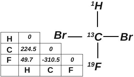
The experiment has been carried out at 300K in $11.7T$ field in a Bruker $AV500$ spectrometer using a triple resonance QXI probe. The system chosen for the implementation of the discrimination algorithm is Carbon-13 labeled Dibromo-fluoro methane ${}^{13}CHFBr_{2}$, where ${}^{1}H$, ${}^{19}F$ and ${}^{13}C$ act as the three qubits[39, 40]. The ${}^{1}H$, ${}^{19}F$ and ${}^{13}C$ resonance frequencies at this field are 500, 470 and 125 MHz, respectively. The scalar couplings between the spins are: $J_{HC}=224.5Hz$, $J_{HF}=49.7Hz$ and $J_{FC}=-310.9Hz$(Fig.3).

The NMR Hamiltonian for a three qubit weakly coupled spin system is [41],

where $\nu_{i}$ are the Larmor frequencies and the $J_{ij}$ are the scalar couplings. The starting point of any algorithm in an NMR quantum information processor is the equilibrium density matrix, which under high temperature and high field approximation is in a highly mixed state represented by[40],

There are several methods for creating pseudo pure states (PPS) in NMR from equlibrium state [42, 43, 10, 44]. We have utilized the spatial averaging technique [10] for creating pseudo pure states as described in [40]. The spectra for equlibrium and $|000\rangle$ PPS are shown in Fig.3.

For Phase Estimation algorithm, due to its high sensitivity, proton spin has been utilized as the ancilla qubit; and the two qubit states, to be discriminated, are encoded in carbon and fluorine spins. As the measurements are performed only on ancilla qubit, we record only proton spectra for non-destructive discrimination of the state of carbon and fluorine. The state of the ancilla qubit can be identified by the relative phase of the spectra. We set the phase such that a positive peak indicates that the proton was initially in state $|0\rangle$.

References

- [1] D Deutsch and R Jozsa. Proceedings of the Royal Society of London A, 439:553, 1992.
- [2] P. Shor. Algorithms for quantum computation: Discrete logarithms and factoring. FOCS, 1994.
- [3] L.K. Grover. American Journal of Physics, 69:769, 2001.
- [4] G. K. Brennen, C. M. Caves, P. S. Jessen, and I. H. Deutsch. Phys. Rev. Lett., 82:1060, 1999.
- [5] J. A. Jones. nmr quantum computation. Prog. NMR Spectrosc, 38:325, 2001.
- [6] M. A. Nielson and I. L. Chuang. Quantum Computation and Quantum Information. Cambridge University Press, 2002.
- [7] F. Schmidt-Kaler, H. Haffner, S. Gulde, M. Riebe, G. P. T. Lancaster, T. Deuschle, C. Becher, W. Hansel, J. Eschner, and C.F. Roos. Appl. Phys. B, 77:789, 2003.
- [8] A. P. Nizovtsev, S. Y. Kilin, F. Jelezko, T. Gaebal, I. Pop, A. Gruber, and J. Wrachtrup. Optics and Spectropy, 99,:233, 2004.
- [9] J. A. Jones and M Mosca. Phys. Rev. Lett., 109:1648, 1998.
- [10] D. G. Cory, M. D Price, and T. F. Havel. Physica D, 120:82, 1998.
- [11] N Linden, H Barjat, and R Freeman. Chemical Physics Letters, 296:61, 1998.
- [12] D. Gottesman and I. L. Chuang. NATURE, 402:390, 1999.
- [13] L. M. K. Vandersypen, M Steffen, G Breyta, C. S Yannoni, M. H. Sherwood, and I. L. Chuang. Nature, 414:883, 2001.
- [14] K Dorai, Arvind, and Anil Kumar. Phys. Review A, 63:034101, 2001.
- [15] R. Das, A. Mitra, S. Vijaykumar, and Anil Kumar. J. of Quantum Information, 3:387, 2003.
- [16] C. Negrevergne, R. Somma, G. Ortiz, E. Knill, and R. Laflamme. Phys. Rev. A, 71:032344, 2005.
- [17] A. Mitra, T. S. Mahesh, and Anil Kumar. J. Chem. Phys., 128:124110, 2008.
- [18] X. Peng, Z. Liao, N. Xu, G. Qin, X. Zhou, D. Suter, and J. Du. Phys. Rev. Lett., 101:220405, 2008.
- [19] A. W. Harrow, A. Hassidim, and S. Lloyd. Phys. Rev. Lett., 103:150502, 2009.
- [20] J. Du, N. Xu, X. Peng, P. Wang, S. Wu, and D. Lu. Phys. Rev. Lett., 104:030502, 2010.
- [21] J. Walgate, A. J. Short, L. Hardy, and V. Vedral. Phys. Rev. Lett., 85:4972, 2000.
- [22] S. Ghosh, G. Kar, A. Roy, A Sen, and U. Sen. Phys. Rev. Lett., 87:277902, 2001.
- [23] S. Virmani, M. F. Sacchi, M. B. Plenio, and D. Markham. Phys. Lett. A, 288:62, 2001.
- [24] X. Y. Chen and D. Yang. Phys.Rev.A, 64:064303, 2001.
- [25] G. Brassard, P. Høyer, and A. Tapp. Quantum counting. ICALP, 1998.
- [26] B. P. Lanyon, J. D. Whitfield, G. G. Gillet, and M. E. Goggin. arXiv:quant-ph/09050887., 2010.
- [27] M. Gupta and P. K. Panigrahi. quant-ph/0504183v1, 2005.
- [28] J. H. Samal, M Gupta, P. K. Panigrahi, and Anil Kumar. J.Phys.B, 43:095508, 2010.
- [29] A Einstein, B Podolsky, and N Rosen. Phys. Rev., 47:777, 1935.
- [30] C.H. Bennett, G. Brassard, C. Crepeau, R. Josza, A. Peres, and W K. Wootters. Phys. Rev. Lett., 70:1895, 1993.
- [31] C. H. Bennett and S.J. Wiesner. Phys.Rev.Lett., 69:2881, 1992.
- [32] J. W. Pan, D. Bouwmeester, H. Weinfurter, and A. Zeilinger. Phys.Rev.Lett., 80:3891, 1998.
- [33] M. Zukowski, A. Zeilinger, M. A. Horne, and A. K. Ekert. Phys.Rev.Lett, 71:4287, 1993.
- [34] A. K. Pati. Phys.Rev.A, 63:014302, 2000.
- [35] D. M. Greenberger, M. A. Hornec, and A. Zeilinger. arXiv:0712.0921v1, 2007.
- [36] J. C. Hao, C. F. Li, and G. C Guo. Phys.Rev. A, 63:054301, 2001.
- [37] L. Xiao, G. L. Long, F. G. Deng, and J. W. Pan. Phys.Rev. A, 69:052307, 2004.
- [38] Y Guo1, shi Shi, and G Zeng. Phys. Scr., 81:045006, 2010.
- [39] L. M. K. Vanedrsypen. Experimental Quantum Computation with Nuclear Spins in Liquid Solution- Doctoral Thesis, page 167, 2001.
- [40] A. Mitra, K. Sivapriya, and Anil Kumar. Journal of Magnetic Resonance, 187:306, 2007.
- [41] R. R. Ernst, G Bodenhausen, and A. Wokaun. Principles of Nuclear Magnetic Resonance in One and Two Dimensions. Oxford University Press, 1990.
- [42] D. G. Cory, A. F. Fahmy, and T. F. Havel. Proc. Natl. Acad. Sci. USA, 94:1634, 1997.
- [43] N Gershenfeld and I. L Chuang. Science, 275:350, 1997.
- [44] T.S. Mahesh and Anil Kumar. Phys. Rev. A., 64:012307, 2001.
- [45] M. H. Levitt and R. Freeman. J. Magn. Reson., 33:473, 1979.
- [46] O. W. Sorensen, G. W. Eich, H Levitt, M, G. Bodenhausen, and R. R Ernst. Prog. in NMR Spectrosc., 16:163, 1984.
- [47] C. H Tseng, S Somaroo1, Y. Sharf, E. Knill, R. Laflamme, T. F. Havel, and D. G. Cory. Phys. Rev. A, 61:012302, 1999.
- [48] A. Mitra, A. Ghosh, R Das, A. Patel, and Anil Kumar. Journal of Magnetic Resonance, 177:285, 2005.