Bosch-Ramon & KhangulyanSecondary Radio emission in -Ray Binaries
Gamma-rays: theory – stars: binaries (including multiple): close – Radiation mechanisms: non-thermal
Monte-Carlo Simulations of Radio Emitting Secondaries in -Ray Binaries
Abstract
Several binary systems that contain a massive star have been detected in both the radio band and at very high energies. In the dense stellar photon field of these sources, gamma-ray absorption and pair creation are expected to occur, and the radiation from these pairs may contribute significantly to the observed radio emission. We aim at going deeper in the study of the properties, and in particular the morphology, of the pair radio emission in gamma-ray binaries. We apply a Monte-Carlo code that computes the creation location, the spatial trajectory and the energy evolution of the pairs produced in the binary system and its surroundings. The radio emission produced by these pairs, with its spectral, variability and spatial characteristics, is calculated as it would be seen from a certain direction. A generic case is studied first, and then the specific case of LS 5039 is also considered. We find that, confirming previous results, the secondary radio emission should appear as an extended radio structure of a few milliarcseconds size. This radiation would be relatively hard, with fluxes up to mJy. Modulation is expected depending on the gamma-ray production luminosity, system eccentricity, and wind ionization fraction, and to a lesser extent on the magnetic field structure. In gamma-ray binaries in general, the pairs created due to photon-photon interactions can contribute significantly to the core, and generate an extended structure. In the case of LS 5039, the secondary radio emission is likely to be a significant fraction of the detected core flux, with a marginal extension.
1 Introduction
High-mass binary systems are a well established class of very high-energy (VHE) gamma-ray emitters. Five VHE sources11 1 There is also the new GeV gamma-ray binary, 1FGL J1018.65856, which may have also been detected at VHE (e.g. [19, 20]). have been associated so far to binaries that contain a massive star: PSR B125963 (Aharonian et al., 2005a); LS 5039 (Aharonian et al., 2005a); LS I +61 303 (Albert et al., 2006); Cygnus X-1 (Albert et al., 2007); and HESS J0632057 (Aharonian et al., 2007; Hinton et al., 2009; Skilton et al., 2009; Falcone et al., 2010; Falcone et al., 2011; Moldón et al., 2011). Among these five, three show clear modulation of the VHE emission associated to the orbital motion: PSR B125963 (Aharonian et al., 2005a), LS 5039 (Aharonian et al., 2006), and LS I +61 303 (Albert et al., 2009); thus, the emitter cannot be too far from the star in these sources. The short duration of the VHE flare observed in Cygnus X-1 (Albert et al., 2007) likely implies that this flare is originated not too far from the star, whereas in HESS J0632057 the situation is less clear (see Skilton et al. (2009); Falcone et al. (2010); Falcone et al. (2011); Moldón et al. (2011)). Under the strong ultraviolet photon field of a massive star, gamma-ray absorption can take place (e.g. Ford (1984); Protheroe & Stanev (1987); Moskalenko & Karacula (1994); Bednarek (2000); Boetcher & Dermer (2005); Dubus (2006a); Boetcher (2007); Orellana et al. (2007); Khangulyan et al. (2008); Reynoso et al. (2008); Sierpowska-Bartosik & Torres (2008); Romero et al. (2010)), this process leading to the creation of secondary (electron-positron) pairs with energies GeV and peaking around 30 GeV.
Secondary pairs are created under the stellar photon field and, as shown below, are likely trapped by the stellar wind magnetic field of strength . For small enough values of and high enough values of the secondary particle energy , most of the pair energy is emitted, via inverse Compton (IC) scattering of stellar photons, as gamma-rays with energies above the pair-creation threshold. If the gamma-ray opacity coefficient is , the electromagnetic cascade may significantly affect the distribution of secondary pairs in the system. However, for this to be efficient the initial gamma-ray energy must be well above the pair creation energy threshold, (i.e. deep in the Klein-Nishina -KN- regime), where , and are the threshold, the gamma-ray and the stellar photon energies in units. In this regime, say for energies of the secondary pairs TeV and typical stellar temperatures K, synchrotron cooling suppresses the cascade under a magnetic field (Khangulyan et al., 2008)
| (1) |
where and are the star luminosity and distance from the star center, respectively. Equation 1 has been derived from Eq. 1 in Khangulyan et al. (2008), which gives the IC cooling timescale in the KN regime with a 10 eV photon field as target. We reproduce the formula here for the sake of clarity:
| (2) |
where is the stellar radiation energy density, and is the electron energy. For , the secondary bolometric luminosity output will be dominated by synchrotron radiation. This implies a magnetic field strength:
| (3) |
All this shows that even for magnetic fields well below equipartition with radiation, synchrotron losses can effectively prevent development of electromagnetic cascades.
Bosch-Ramon et al. (2008a) carried out a detailed semi-analytical study of the spectral properties of the secondary broadband emission for realistic magnetic field values (see also Bosch-Ramon et al. (2008b)). In that work, it was shown that the radio, X-ray, and GeV fluxes of secondary emission could be comparable to those observed in gamma-ray binaries, and may even dominate the non-thermal output below in some cases. These authors also suggested that the extended radio emission found in LS I +61 303 (Dhawan et al., 2006) may come from secondary pairs. Bosch-Ramon (2009) also proposed this origin for the emission of the marginally resolved radio core of LS 5039 (Ribó et al., 2008).
Although the radio fluxes can be roughly estimated from the semi-analytical study of Bosch-Ramon et al. (2008a), their approach does not allow a proper description of the radio spectrum, lightcurve, and morphology, because synchrotron radio emitting particles have long timescales and are strongly affected by the medium inhomogeneity at spatial scales of . In that work, the complex 3-dimensional (3D) structure of the secondary trajectories was simplified attaching the secondary pairs to the stellar wind, with the latter being taken as spherically symmetric, with constant velocity, and wind particle and magnetic field energy density . The magnetic field was considered fully irregular. Finally, the adiabatic cooling of the secondary pairs was not taken into account, which is reasonable at binary spatial scales, but not for the computation of that radio emission produced outside the binary system, affected by wind expansion. Finally, the relevance of free-free absorption was not investigated.
In this work, we present detailed calculations of the evolution of the radio emitting secondary pairs in gamma-ray binaries. The energy and the spatial evolution of the particles in the stellar wind have been computed using a Monte-Carlo code that accounts for ionization/coulombian collision losses, adiabatic, relativistic bremsstrahlung, synchrotron, and IC cooling, as well as diffusion and advection in the wind to follow the trajectories of secondary pairs in the source. The code can also deal with anisotropic diffusion when an ordered magnetic field is dominant, although we do not consider this configuration at this stage. A sketch of the the scenario at the scales of the binary system is shown in Fig. 1. Once the particle energy and spatial distributions have been obtained at a particular orbital phase (accounting for the previous orbital history of the system), the radio emission in a specific direction is calculated, which allows the generation of directional radio maps. The radio maps have been smoothed using a circular Gaussian in order to roughly reproduce what an observer would see using a milliarcsecond (mas) resolution radio interferometer. This is also illustrated in Fig. 1. Spectra and lightcurves, and the impact of free-free absorption, have been discussed. We focus here on a generic case, since our aim is to give a general demonstration of the relevance of secondary radio emission, but we provide also with an instance of the importance of this phenomenon in a real source, applying our calculations to LS 5039. Further and more detailed studies for specific objects of the role of secondary pairs for the radio emission will be presented elsewhere.


2 Monte-Carlo simulations of secondary pairs in gamma-ray binaries
For an appropriate study of the secondary radio emission, detailed calculations of the energy and spatial evolution of the secondary pairs are required, accounting for the star radiation field and the properties of the stellar wind. Given the difficulties of treating the magnetic field structure and adiabatic cooling in the wind in a semi-analytical approach, we have performed Monte-Carlo simulations in which secondaries pairs are injected, move (diffuse and are advected), and cool down in a 3D space.The 3D nature of the problem comes from the combination of the advection in the wind plus the orbital motion (a significant regular -field structure would also require a 3D treatment). The problem treated by the Monte-Carlo method is similar to that described by the diffusion advection equation (e.g. Jones (1990); Blandford & Eichler (1987)). The radiation timescales (, where is the electron energy loss rate) adapted to the environments of gamma-ray binaries are:
| (4) |
| (5) |
| (6) |
for synchrotron, IC (Thomson) and relativistic Bremsstrahlung, respectively (see Bosch-Ramon & Khangulyan (2009) for the IC cooling rate accounting also for the KN regime used in the calculations), with being the wind density (see below), the energy density of the target photon field, and the ambient magnetic field. For the adiabatic and ionization cooling timescales, we have adopted:
| (7) |
and
| (8) | |||||
respectively, where is the wind velocity at infinity, and the stellar radius.
2.1 Injection of secondary pairs in the binary system
We have calculated the injected spatial and energy distribution of secondary pairs for a given primary gamma-ray spectrum and a stellar black-body photon field. This is done tracking the path of a photon produced in the emitter location and moving with a certain direction in the binary system. The location in which a given gamma ray is absorbed is obtained using the (anisotropic) gamma-ray absorption differential probability due to photon-photon interactions (point-like treatment of the star; see below):
| (9) |
where , , and are the length of the path covered by the gamma ray, the gamma-ray/stellar photon interaction angle, the stellar photon specific density, and the pair-creation cross section (Gould & Schréder, 1967), respectively. This quantity is integrated along the photon path to obtain the probabity of interaction up to a certain location. In this work, the absorption probability is computed along the photon trajectory with small steps, and the Monte-Carlo algorithm is applied to define the interaction point.
The injection rate of secondary pairs depends strongly on the spectrum and angular distribution of the primary gamma rays. To mimic the effect of the anisotropic IC scattering in the angular distribution of primary gamma rays, a gamma-ray direction probability at injection has been introduced, where is the angle between the gamma-ray path and the direction from the star to the gamma-ray emitter, i.e. gamma rays have a higher probability to be emitted towards than away from the star. This angular dependence would roughly correspond to an average one between the Thomson and KN IC regimes (see Fig. 6 in Khangulyan et al. (2008)).
In Fig. 2, we show the distribution of injected secondary pairs in a gamma-ray binary for three different energies. We have focused here on a generic case, in which we have adopted a circular binary system () of one week period, formed by a massive, primary star of mass and compact object of mass , such that . This yields an orbital separation distance of cm. The inclination of the system has been fixed to , and the phase 0.0/0.5 has been taken at the superior/inferior conjunction of the compact object (supc/infc). The main star parameters have been fixed to erg s-1, cm and K, where is the star temperature. The gamma-ray emitter has been assumed to be point-like, at the compact object location, with , although the actual location and size of the VHE emitter in gamma-ray binaries has not been defined yet, being possible to have an extended production region not only in the jet but also in the colliding wind scenario (see, e.g., Bogovalov et al. (2008)). No eccentricity and a fixed -value have been taken for the sake of simplicity, since our aim is to illustrate the main characteristics of the secondary radio emitter.

2.1.1 Treatment of the star
In these calculations, we have adopted a point-like approximation for the star (e.g. Dubus (2006a); see also Sect. 4.2.1 in Bosch-Ramon & Khangulyan (2009)). This approximation fails close to the stellar surface, at a distance comparable to the radius of the star , i.e. . This region will be relevant for gamma rays with pair-production mean-free paths comparable to the distance between the star and the gamma-ray emitter. Such gamma rays can be absorbed in a volume , with a sub-region affected by the star finite-size of volume . Thus, even for the most sensitive interval of gamma-ray energies, the point-like approximation of the stellar photon field fails for a fraction of the total relevant volume and for and , respectively. Therefore, given a rather broad distribution of primary gamma rays and for , the point-like approximation for the star would have an accuracy at least of the order of a 10%. This estimate is suported by semi-analytical calculations of the pair injection rate density, whose results are presented in Fig. 3. The calculation is done computing first the gamma-ray flux that reaches a certain point in the binary system. Then, the rate density of pairs of 100 GeV (dominant in radio) injected in each point is computed, accounting for the energy differential cross section of pair creation (see Bosch-Ramon et al. (2008a) and references therein). This calculation have been performed for a generic case and for LS 5039 (see Table 2). In Fig. 4, we show the fraction of primary gamma-rays absorbed in the system, as a function of the gamma-ray energy, for two different distances between the gamma-ray emitter and the star: and , with the properties of the star chosen as in the generic case. As seen from these figures, accounting the stellar finite size or adopting a point-like star approximation yield almost the same results. This permits to safely adopt the point-like approximation for the Monte-Carlo calculations presented below, shortening significantly the calculation time.


2.1.2 Primary gamma-ray spectrum and flux
To perform the calculations corresponding to a generic gamma-ray binary, the photon index of the produced gamma rays has been taken , and the unabsorbed differential photon rate at 1 TeV is TeV-1 s-1, which corresponds to a specific photon flux TeV-1 s-1 cm-2 at a distance of kpc. These values are assumed to be orbital phase independent. In Fig. 5, we show the primary gamma-ray emission between 20 GeV to 2 TeV in the observer direction, for the orbital phases 0.0 (supc), 0.25, 0.5 (infc), and 0.75. The thin lines correspond to the intrinsic spectra, whereas the thick ones take into account photon-photon absorption. The computed absorbed specific photon fluxes are, at 1 TeV: (phase 0.0), (phase 0.25/0.75) and TeV-1 s-1 cm-2 (phase 0.5).

2.2 Energy and spatial evolution of secondary pairs
2.2.1 Transport of secondary pairs
A secondary pair is injected where the gamma ray was absorbed, and the subsequent locations are computed accounting for the local direction and strength of the wind magnetic field, which is assumed to have an ordered and a disordered component. We consider the stellar rotation axis to be perpendicular to the orbital plane.
The ordered wind magnetic field can be described as , where
| (10) |
| (11) |
and and are the magnetic field at the star surface and the initial azimuthal wind velocity, respectively. For the calculations, is fixed to a value of 200 G (see Bosch-Ramon et al. (2008b) and references therein), high enough to suppress the electromagnetic cascade. We neglect here the region within the Alfven radius from the star, typically confined to a region , since almost all secondary pairs are created farther from the star. The wind velocity can be expressed as , where:
| (12) |
and the azimuthal one:
| (13) |
The wind density depends on as
| (14) |
where is the star mass-loss rate. In this work, we have taken yr-1 and cm s-1. The magnetic field and the wind model adopted here are based on that presented in Usov & Melrose (1992).
The irregular component of the magnetic field, , allows particles to effectively diffuse in the stellar wind. The particle mean free paths parallel and perpendicular to the magnetic lines are and , where is the electron gyro radius, and is and relates the irregular and the wind magnetic field component through . (thus the ordered component strength is ). The spatial power spectrum of is assumed to be flat, i.e. does not depend on energy, and the diffusion coefficients are proportional to the Bohm one: .
The diffusion approximation is applicable if secondary pairs deflect significantly before cooling down, i.e. :
| (15) |
In addition, the particle mean free path parallel to the magnetic lines (always longer than the perpendicular one) should be much smaller than the system typical scale :
| (16) | |||||
The simulation time steps have to fulfill as well these conditions and in addition be for the diffusion approximation to be suitable. All this has been accounted for in the calculations.
The diffusion in the stellar wind has been accounted in each step of the secondary evolution as a location shift, , which corresponds to the diffusion displacement vector of the particle after a time interval , accounting for the diffussion coefficients . Since particles are confined to the stellar wind, they will be also advected by the wind. This advection motion has been accounted for introducing an additional shift in the particle location after each time step by . The total spatial shift of the secondary location per time step is therefore .
For the sake of simplicity, at this stage we have assumed a fully disordered magnetic field with . We note that, as long as , i.e. for (see Eq. 16), radio emitting secondary pairs will basically move anchored to the stellar wind. In Table 1, the parameter values are given for the generic case studied in this work.
| Parameter [units] | Symbol | Value |
| Stellar radius [cm] | ||
| Orbit separation distance [cm] | ||
| Emitter-to-star distance [cm] | ||
| Stellar temperature [K] | ||
| total system mass [] | 22 | |
| Star surface magnetic field [G] | 200 | |
| Mass-loss rate [ yr-1] | ||
| Wind speed at infinity [cm s-1] | ||
| Distance [kpc] | 2 | |
| Superior conjunction | supc | 0.0 |
| Inferior conjunction | infc | 0.5 |
| Inclination angle [∘] | 45 | |
| Irregular magnetic field fraction | 1 | |
| 1 TeV specific flux [TeV-1 s-1] | ||
| Gamma-ray photon index | 2.5 | |
2.2.2 Secondary particle energy evolution
Once created at time , the secondary pair trajectory is calculated by the Monte-Carlo code up to time , i.e. the time when the energy and spatial distributions of pairs and their radiation are computed. The energy evolution of secondary pairs is calculated accounting for the energy losses along the trajectory taking into account all the processes in play: ionization, adiabatic, relativistic bremsstrahlung, synchrotron, and IC cooling. Thus, at each time step , a certain amount of energy is rested to the particle energy at , where is such that , and includes the cooling mechanisms specified above. We note that the energy losses depend not only on the particle energy, but also on the particle position in the system.
In the region close to the star ( few ), IC cooling dominates for basically all the particle energies, although at this distance there are none or very few radio emitting particles. Farther out, adiabatic cooling in the wind becomes faster. The energy distribution of radio secondaries almost does not depend on the original gamma-ray spectrum, since radio emitting secondary pairs are mostly produced around and then cool down. Dominant IC cooling yields an electron energy distribution below the pair creation threshold , whereas adiabatic cooling renders .
In the Monte-Carlo simulation we have considered an equal number of primary gamma-rays ( and for the generic and LS 5039 cases, respectively) per logarithmic energy bin with the angular distribution described in Sect. 2.1. The injection process has been implemented during the relevant time interval, starting early enough before the time , to account for all the relevant secondary pairs (say, at ). The orbital motion of the primary gamma-ray source has been accounted in the calculations of the injection rate. The Monte-Carlo code calculates the secondary pair energy and space distribution at the time keeping record of the time of creation and the initial pair energy. To compute the final radiative output of the secondary pairs one has to account for the adopted gamma-ray injection spectrum () and the corresponding normalization, i.e. one needs to know how many particles correspond in reality to one particle of the simulation.
An analytical code has been used to compute the total amount of secondary pairs generated per energy bin for the primary gamma-ray distribution . This value, divided by the number of secondary particles per energy bin injected in the simulation, gives the weight of an electron/positron from the evolved distribution of particles. This weight depends on the secondary particle energy, and may vary with the orbital phase, i.e. with injection time .
Pairs created at different epochs can contribute to the radio emission at the same frequency at the final time , since pairs may have different initial energies and spatial trajectories and therefore cooling times differ as well.
In Figs. 6 and 7, we show the (evolved) secondary location distribution and density map, respectively, projected in the observer plane for four different phases, 0.0, 0.25, 0.5, and 0.75.


2.3 Secondary pair radiation
From the energy and the spatial distribution of particles at a specific orbital phase, we have computed the synchrotron emission convolving the particle energy distribution with the one-particle power function. Computing the fluxes from 2D small regions or bins in the observer plane (image pixels), i.e. integrating in depth, permits to extract radio morphologies. The radio emission has been calculated in the optically thin approximation of synchrotron radiation, valid at frequencies above few GHz for the relevant spatial scales. For a 10 mJy source with the self-absorption turnover at GHz, the radio emitter size would be constrained to cm (Bosch-Ramon, 2009) (where would be the radio emitter characteristic magnetic field), or mas at few kpc.
Typical radio fluxes of about 20 mJy are obtained at 5 GHz for the parameter values adopted here. Note that, fixing , the secondary radio flux is . The spectral shape of the specific flux is almost flat, constant, since adiabatic losses dominate the secondary pair evolution. Part of the radio emission originates nevertheless in regions in which IC cooling dominates, which softens the spectrum. Free-free absorption, of coefficient , could be relevant. Adopting a simple prescription for which does not depend on the orbital phase in a circular orbit (see Eq. 1 in Bosch-Ramon (2009), adapted from Rybicki & Lightman (1979)), we find that for ionization fractions , the radio fluxes should be already significantly affected. Another effect of the free-free absorption is a strong spectral hardening, although for a combination of the energy and the spatial distribution of secondaries yields again a flat spectrum. All this is shown in Fig. 8. Regarding the magnetic field geometry, fixing implies that the synchrotron power does not depend on the magnetic field orientation and therefore the orbital phase. For , changes in the -line of sight angle could introduce moderate orbital flux variability. For a dominantly toroidal magnetic field, synchrotron flux variations would be of the order of (2 for ), with two dips and two enhancements along the orbit when the -line of sight angle reached and , respectively.

The radiation image can be computed as it would be seen by the observer projecting the 3D emitter in the observer plane and dividing then in 2D bins. From that, synthetic radio maps can be produced convolving the fluxes in these bins with a circular Gaussian of full width half maximum (FWHM) of 1 mas. The result will be similar to an image obtained by a radio interferometer with angular resolution of 1 mas. In Figs. 9, 10 and 11, we show three sets of 5 GHz radio images at four different phases: 0.0 (supc), 0.25, 0.5 (infc), and 0.75. Fig. 9 corresponds to the raw image, i.e. without Gaussian convolution. There is an expectable similarity in shape between the radio secondary (Fig. 7) and the flux spatial distribution. The image convolved with a Gaussian with FWHM=1 mas is presented in Fig. 10, and Fig. 11 shows the residuals when extracting a point-like source (the FWHM=1 mas Gaussian) to the convolved image both with the same flux. Typical noise levels for such an interferometer could be mJy/beam, slightly below the predicted excesses (see the intensity scale in Fig. 11). The impact of free-free absorption has not been included in these plots, which would consist on a reduction of the fluxes in the image core but keeping an excess in the periphery.


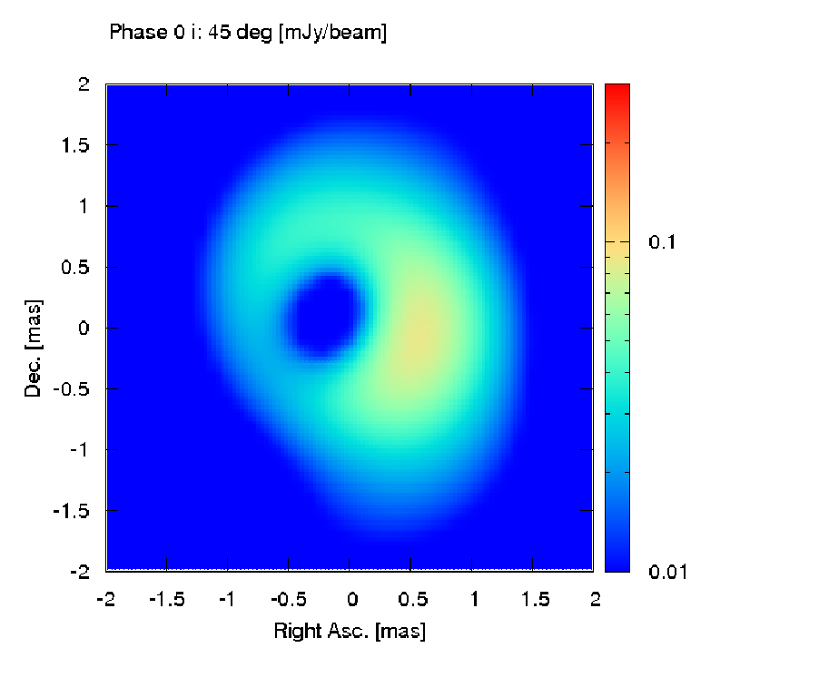
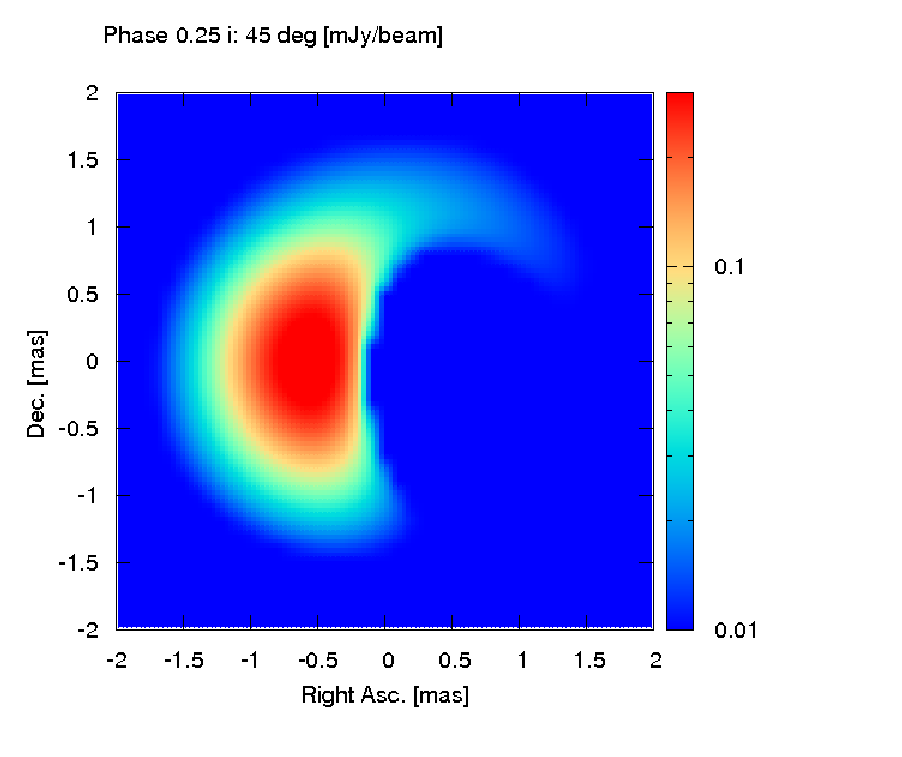

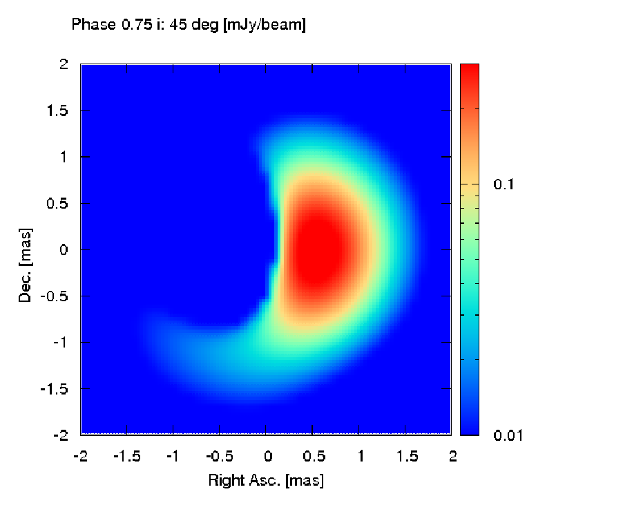
We have focused in this work on the synchrotron radio emission. We note nevertheless that for the parameter values adopted here, the synchrotron X-ray and IC GeV fluxes would be both about few erg s-1 cm-2. A more detailed study of the higher energy secondary radiation will be presented elsewhere.
3 Application to LS 5039
We have applied our Monte-Carlo code and radiation model presented above to LS 5039. LS 5039 is a high-mass X-ray binary, detected in VHE gamma rays (Aharonian et al., 2005b; Aharonian et al., 2006), which has been observed in radio with different VLBI instruments for more than a decade (Martí et al., 1998; Paredes et al., 2000; Paredes et al., 2002; Ribó et al., 2008). The work by Ribó et al. (2008) presents VLBA observations at 5 GHz in which the radio core appears as marginally resolved, with two small dipolar elongated extensions that show a moderate change in the position angle. The core and extension fluxes are 18–20 mJy and 6–4 mJy, respectively, having the whole structure an angular size of several mas. The radio structures found in the source have been associated either to a jet (Paredes et al., 2000) or a shocked pulsar wind (Dubus, 2006b). The binary system consists of an O6.5 main sequence star and a compact object of unclear nature (neutron star or black hole; see Casares et al. (2005)). The system semi-major axis is cm, with eccentricity and orbital period days. The phase 0.0 corresponds to the periastron passage, and phases 0.05 and 0.67 to supc and infc of the compact object, respectively. The inclination angle of the orbit is not known and could be in a range between . The stellar mass-loss rate has been taken to be yr. The ephemeris, orbital parameters, system-observer geometry, star and stellar wind properties, and inclination angle constraints have been taken from Casares et al. (2005) and Aragona et al. (2009) (see also Sarty et al. (2010)). The system orientation in the plane of the sky, unconstrained from observations, has been taken as in Fig. 6 of Aragona et al. (2009). Following the approach for the generic case, has been fixed to (though our results should not change qualitatively for values ). The values of and have been taken also as in the generic case, 200 G and 1, respectively. The parameters adopted for LS 5039 are presented in Table 2.
Given the uncertainties in the source properties, and the known complexities of the orbit and VHE flux/photon-index lightcurve, we do not aim in this section at carrying a thorough analysis of the different possibilities, what is left for future work. Otherwise, we intend to give two possible instances of the source behavior, and for that we focus on two phases, 0.2, slightly after supc, and 0.8, slightly after infc. The distribution of the gamma rays injected in the system has been chosen such that the source should show absorbed fluxes and photon indices similar to the observed ones (Aharonian et al., 2006) in the direction to the observer. For this, we have deabsorbed the observed VHE spectra (see, e.g., Boetcher (2007)) assuming a point-like emitter in a certain location, as explained below, emitting in the energy range from 20 GeV up to 2 TeV. Since the observed lightcurve shows a relatively smooth behavior around phases 0.45–0.9 and 0.9–0.45 (Aharonian et al., 2006), for simplicity we have adopted typical specific fluxes and photon indices to compute the radio emission: TeV-1 s-1 cm-2 and (phase 0.2), and TeV-1 s-1 cm-2 and (phase 0.8). Since the location of the emitter is not well constrained (Khangulyan et al., 2008; Bosch-Ramon et al., 2008b), two different heights have been chosen that optimize the radio fluxes without entering in strong conflict with the X-ray fluxes. At phase 0.2, we have located the emitter at a height of cm, and at cm at phase 0.8, perpendicularly to the orbital plane, in the observer side of that plane. There is no additional emitter assumed at a location symmetric with respect to the orbital plane, although if gamma-rays were produced in a symmetric bipolar jet, this component should be also included in the calculations. However, given the expected higher wind free-free opacity for this component, its contribution is expected to be smaller than the one considered here. We have computed the secondary injection and evolution starting a phase interval of 0.5 earlier than the phases in which the radiation is evaluated, i.e. and . However, most of the radio emission, including the outermost region of the emitter, comes from secondary pairs injected within a phase interval of 0.2 earlier, due to adiabatic cooling.
The resulting images of the raw radio emission, of the source convolved with a Gaussian, and the residuals after extracting a point-like source are presented in Fig. 12. The figure shows that the radiation, with a typical emitter size of mas, would be difficult to resolve, although the bigger size of the system around infc may lead to a marginal extension. The obtained total fluxes at 5 GHz are about 6 and 10 mJy at phases 0.2 and 0.8, respectively. The complex flux evolution along the orbit of the primary (deabsorbed) gamma-ray spectra yield different spectra from those of the generic case, obtaining (0.2) and (0.8). This is due to secondary pairs injected at different phases, with different absorbed luminosities, produce the radiation at different frequencies at the same orbital phase. The computed luminosities in the range 1–10 keV are of about erg s-1, similar to those observed in this energy range (e.g. Bosch-Ramon et al. (2007); Takahashi et al. (2009)). These X-ray fluxes already constrain the fluxes of the radio emission to several mJy at most. These results are nevertheless sensitive to the radial profile of , which is not well known, thus we do not treat here the high-energy output of the secondary emission. The impact of free-free absorption in the wind has not been considered either, but this process could reduce significantly the secondary radio emission mainly for phases around supc under high ionization fractions.
| Parameter [units] | Symbol | Value |
| Stellar radius [cm] | ||
| Orbital semi-major axis [cm] | ||
| eccentricity | 0.34 | |
| Stellar temperature [K] | ||
| total system mass [] | 25 | |
| Star surface magnetic field [G] | 200 | |
| Mass-loss rate [ yr-1] | ||
| Wind speed at infinity [cm s-1] | ||
| Distance [kpc] | 2.5 | |
| Superior conjunction | supc | 0.05 |
| Inferior conjunction | infc | 0.67 |
| Inclination angle [∘] | 45 | |
| Irregular magnetic field fraction | 1 | |


4 Discussion
This work shows that the radio emission detected from compact gamma-ray binaries that contain a massive star could have a non-negligible component coming from the secondary pairs created in the vicinity of the gamma-ray emitter. Actually, the following simple estimate of the radio flux already indicates this. Assuming that secondary pairs cool mainly through adiabatic cooling in the region in which they produce radio emission, which is the case for a wide range of parameter values, and a wind velocity of cm s-1, the expected fluxes can be derived from the formula:
| (17) | |||||
where is the energy of the radio emitting particles, the angle averaged opacity at gamma-ray energies around 100 GeV, the synchrotron cooling timescale, GeV the secondary typical injection energy, the VHE luminosity, , and the distance to the source. In Eq. (17), the product should be substituted by for (and fixed to 1). In sources with parameters such that mJy, secondary radio emission should not be neglected. The most crucial point here is whether magnetic fields of the order of 10 G can be found at few from the star.
As shown in this work, secondary radio emission from gamma-ray binaries would not be only relevant in flux, but they could also present resolvable extensions. In general, the spectra can be flat or softer depending on (adiabatic vs IC cooling dominance), and the absorbed gamma-ray luminosity and the radio emitter conditions, in particular and , along the orbit. In the particular case of LS 5039, we find that a dominant fraction of the marginally extended core of LS 5039 (Ribó et al., 2008) could be of secondary origin, with a changing relatively soft spectrum. Since the computed additional extension appears marginal, the observed elongated emission at 5 GHz beyond the core in LS 5039 would be likely related to an intrinsic primary radio emitter.
Regarding morphology, we find that a spiral-like shape would be expected, although typically the small angular size of the radio source presently prevents detailed imaging. Such a spiral-like shape was also predicted in Bosch-Ramon et al. (2008a), although the treatment there was simpler than in the present work. It is worthy noting that the wind conditions could differ from those adopted here, and then the shape, and even the radio emitter extension, may change. More collimated radio structures, or a magnetic field increase downstream the wind leading to more extended radio emission, cannot be discarded.
It is remarkable that the spatial distribution of the radio emitting secondary pairs is strongly determined by their injection, which depends on the stellar photon field and the gamma-ray emitter location, and by the stellar wind inhomogeneities and anisotropies, but not by . Only a very regular , with very large -values, could modify significantly the distribution of radio emitting secondary pairs, since then these particles would move at along the dominantly toroidal , i.e. leaving the system with a speed , between and . For reasonable and -values, particles are trapped in the wind, and their energy distribution is determined by IC and adiabatic cooling. The magnetic field strength is then relevant only for the synchrotron fluxes (recall ), and its level of (ir)regularity, , for variability. Polarization would also be affected by , and polarization observations may probe the geometry. However, the high density of cold free electrons in the stellar wind could induce strong Faraday rotation. A proper study of the impact of this on the final polarization degree and angle requires a devoted investigation.
System eccentricity, a significant regular magnetic field component, and free-free absorption would be sources of radio variability and should be considered when studying specific cases. Changes in the gamma-ray luminosity would also lead to a smooth modulation of the secondary radio emission. To finish with, it seems likely that in gamma-ray binaries, the radio emission from inner regions can be, if not dominated, significantly contaminated by secondary radiation. Secondary pairs should not be neglected when understanding the broadband non-thermal emission in compact gamma-ray sources, nor the physical connection of the radiation produced in different bands.
We thank an anonymous referee for her/his many constructive and useful comments and suggestions. The research leading to these results has received funding from the European Union Seventh Framework Programme (FP7/2007-2013) under grant agreement PIEF-GA-2009-252463. V.B-R. acknowledges support by the Ministerio de Educación y Ciencia (Spain) under grant AYA 2007-68034-C03-01, AYA2010-21782-C03-01 and FPA2010-22056-C06-02. V.B-R. thanks Max Planck Institut fuer Kernphysik for its kind hospitality and support. V.B-R. wants to thank the Insituto Argentino de Astronomía and the Facultad de Ciencias Astronómicas y Geofísicas de la Universidad de La Plata for their kind hospitality.
References
- Aharonian et al. (2005a) Aharonian, et al. 2005a, A&A, 442, 1
- Aharonian et al. (2005b) Aharonian, et al. 2005b, Science, 309, 746
- Aharonian et al. (2006) Aharonian, F. A. et al. 2006, A&A, 460, 743
- Aharonian et al. (2007) Aharonian, F. A. et al. 2007, A&A, 469, L1
- Albert et al. (2006) Albert, J. et al. 2006, Science, 312, 1771
- Albert et al. (2007) Albert, J. et al. 2007, ApJ, 665, L51
- Albert et al. (2009) Albert, J. et al. 2009, ApJ, 693, 303
- Aragona et al. (2009) Aragona, C., McSwain, M. V., Grundstrom, E. D., et al. 2009, ApJ, 698, 514
- Bednarek (2000) Bednarek, W. 2000, A&A, 362, 646
- Boetcher (2007) Böttcher, M. 2007, Astr. Phys., 27, 278
- Boetcher & Dermer (2005) Böttcher, M., Dermer, C. D. 2005, ApJ, 634, L81
- Bogovalov et al. (2008) Bogovalov, S. V., Khangulyan, D. V., Koldoba, A. V., Ustyugova, G. V., & Aharonian, F. A. 2008, MNRAS, 387, 63
- Bosch-Ramon et al. (2007) Bosch-Ramon, V., Motch, C., Ribó, M. 2007, A&A, 473, 545
- Bosch-Ramon et al. (2008a) Bosch-Ramon, V., Khangulyan, D., Aharonian, F. A. 2008a, A&A, 482, 397
- Bosch-Ramon et al. (2008b) Bosch-Ramon, V., Khangulyan, D., Aharonian, F. A. 2008b, A&A, 489, L21
- Bosch-Ramon (2009) Bosch-Ramon, V. 2009, A&A, 493, 829
- Bosch-Ramon & Khangulyan (2009) Bosch-Ramon, V. & Khangulyan, D. 2009, Int. Jour. Mod. Phys. D, 18, 347 [astro-ph/0805.4123]
- Casares et al. (2005) Casares, J., Ribó, M., Ribas, I., et al. 2005, MNRAS, 364, 899
- Corbet et al. (2011) Corbet, R. H. D., Cheung, C. C., Kerr, M., 2011, ATel, 3221, 1
- de Ona Wilhelmi (2010) de Ona Wilhelmi, E. for the HESS collaboration, 2010, 38th COSPAR Scientific Assembly, Bremen, Germany, p.6
- Dhawan et al. (2006) Dhawan, V., Mioduszewski, A., & Rupen, M. 2006, in Proc. of the VI Microquasar Workshop, Como-2006
- Dubus (2006a) Dubus, G. 2006, A&A, 451, 9
- Dubus (2006b) Dubus, G. 2006b, A&A, 456, 801
- Blandford & Eichler (1987) Blandford, R., Eichler, D., 1987, Phys. Rep., 157, 1
- Falcone et al. (2010) Falcone, A. D., Grube, J., Hinton, J., et al. 2010, ApJ, 708, L52
- Falcone et al. (2011) Falcone, A., Bongiorno, S., Stroh M., Holder, J. 2011, ATel 3152
- Ford (1984) Ford, L. H. 1984, MNRAS, 211, 559
- Gould & Schréder (1967) Gould, R. J. & Schréder, G. P. 1967, Phys. Rev., 155, 1404
- Hinton et al. (2009) Hinton, J. A., Skilton, J. L., Funk, S., et al. 2009, ApJ, 690, L101
- Jones (1990) Jones, F. C. 1990, ApJ, 361, 162
- Khangulyan et al. (2008) Khangulyan, D., Aharonian, F., & Bosch-Ramon, V. 2008, MNRAS, 383, 467
- Martí et al. (1998) Martí, J., Paredes, J. M., & Ribo, M. 1998, A&A, 338, L71
- Moldón et al. (2011) Moldón, J., Ribó, M., Paredes, J. M. 2011, ATel, 3180, 1
- Moskalenko & Karacula (1994) Moskalenko I. V., Karakula S., 1994, ApJ, 92, 567
- Orellana et al. (2007) Orellana, M., Bordas, P., Bosch-Ramon, V., Romero, G. E., & Paredes, J. M. 2007, A&A, 476, 9
- Paredes et al. (2000) Paredes, J. M., Martí, J., Ribó, M., & Massi, M. 2000, Science, 288, 2340
- Paredes et al. (2002) Paredes, J. M., Ribó, M., Ros, E., Martí, J., & Massi, M. 2002, A&A, 393, L99
- Protheroe & Stanev (1987) Protheroe, R. J. & Stanev, T. 1987, ApJ, 322, 838
- Reynoso et al. (2008) Reynoso, M. M., Christiansen, H. R., & Romero, G. E., 2008, Astrop. Phys. 28, 565
- Ribó et al. (2008) Ribó, M., Paredes, J. M., Moldón, J., Martí, J., Massi, M. 2008, A&A, 481, 17
- Romero et al. (2010) Romero, G. E., del Valle, M. V., & Orellana, M. 2010, A&A, 518, 12
- Rybicki & Lightman (1979) Rybicki, G. B., & Lightman, A. P. 1979, Radiative processes in astrophysics (New York: Wiley-Interscience)
- Sarty et al. (2010) Sarty, G. E., Szalai, T., Kiss, L. L. 2010, MNRAS, in press [astro-ph/1009.5150]
- Sierpowska-Bartosik & Torres (2008) Sierpowska-Bartosik, A. & Torres, D. F., 2008, APh, 30, 239
- Skilton et al. (2009) Skilton, J. L., Pandey-Pommier, M., Hinton, J. A., et al. 2009, MNRAS, 399, 317
- Takahashi et al. (2009) Takahashi, T., Kishishita, T., Uchiyama, Y., et al. 2009, ApJ, 697, 592
- Usov & Melrose (1992) Usov, V. V.,& Melrose, D. B. 1992, ApJ, 395, 575