On relaxing the constraints in pairwise compatibility graphs
Abstract
A graph is called a pairwise compatibility graph (PCG) if there exists an edge weighted tree and two non-negative real numbers and such that each leaf of corresponds to a vertex and there is an edge if and only if where is the sum of the weights of the edges on the unique path from to in . In this paper we analyze the class of PCG in relation with two particular subclasses resulting from the the cases where (LPG) and (mLPG). In particular, we show that the union of LPG and mLPG does not coincide with the whole class PCG, their intersection is not empty, and that neither of the classes LPG and mLPG is contained in the other. Finally, as the graphs we deal with belong to the more general class of split matrogenic graphs, we focus on this class of graphs for which we try to establish the membership to the PCG class.
keywords: PCG, leaf power graph, threshold graphs, matrogenic graphs.
1 Introduction
Given an edge weighted tree , let and be two nonnegative real numbers with . For any two leaves and of the tree , we denote by the sum of the weights of the edges on the unique path from to in . Starting from , and , it can be easily constructed a pairwise compatibility graph of , i.e. a graph where each vertex corresponds to a leaf of and there is an edge if and only if . We will denote such a graph by . Consequently, we say that a graph is a pairwise compatibility graph (PCG) if there exists an edge weighted tree and two nonnegative real numbers and such that . Determine whether a graph is a PCG seems in general difficult even if at the beginning, when the problem arose in a computational biology context [3], it was conjectured that every graph was a PCG. Nowadays it is known that this conjecture is false [6], while it is proved that some specific classes of graphs e.g., graphs with five nodes or less [5], cliques and disjoint union of cliques [2], chordless cycles and single chord cycles [7] and some particular subclasses of bipartite graphs [6], are PCG.
The pairwise compatibility concept is defined with respect to two bounds concerning and . If we relax these conditions, requiring only that the distance between some pair of leaves is smaller than or equal to (i.e. we set ) then we are considering a particular subclass of PCG graphs, namely the leaf power graphs (LPG). More formally, a graph is a leaf power if there exists a tree and a nonnegative number such that there is an edge in if and only if for their corresponding leaves we have (see [4]). Although there has been a lot of works on this class of graphs [2], a completely description of leaf power graphs is still unknown.
To the best of our knowledge, nothing is known in literature concerning the subclass of PCG when the constraint concerns only the minimum distance, i.e. there is an edge in if and only if the corresponding leaves are at a distances greater than in the tree (observe that in this case we set ). In this paper we introduce this new concept and exploit the relations between the new defined class and the two known classes LPG and PCG.
The paper is organized as follows: in Section 2 we introduce some terminologies and recall some known concepts that we will use in the forthcoming work. Then, we define the new subclass of PCG, namely mLPG, characterized by the use of only. Next, in Section 3 we study the relations between the classes PCG, LPG and mLPG. In particular, we show that the union of LPG and mLPG does not coincide with the whole class PCG, their intersection is not empty, and neither of the classes LPG and mLPG is contained in the other. All the graphs we furnish as examples in Section 3 are particular cases of the more general class of split matrogenic graphs. Hence, in Section 4 we focus on the class of split matrogenic graphs trying to determine if it belongs to the PCG class. We prove that many split matrogenic graphs are PCG. However, the membership to PCG class of one particular subclass of split matrogenic graph remains an open problem that is reported in the final Section 5 together with some other open problems.
2 Preliminaries
In this section we introduce some definitions and some concepts that we use in the rest of this paper.
When we say that a tree is weighted, we mean that it is edge weighted, that is each edge is assigned a number as its weight. In this paper we consider only weighted trees and graphs that are connected.
A caterpillar is a tree in which all the vertices are within distance one of a central path which is called the spine.
A graph is said to be split if there is a vertex partition such that the subgraphs induced by and are complete and stable, respectively.
Given two split graphs and their composition is formed by taking the disjoint union of and and adding all the edges such that and . Observe that is again a split graph.
A set of edges is a perfect matching of dimension of onto if and only if and are disjoint subsets of vertices of cardinality and each vertex in is adjacent to exactly one vertex in and no two edges share a point. We say that the split graph is a split matching if the subset of edges in not belonging to the clique forms a perfect matching. We denote by the class of split matching graphs.
An antimatching of dimension of onto is a set of edges such that the non edges between and form a perfect matching. We say that the split graph is a split antimatching if the subset of edges in not belonging to the clique forms an antimatching. We denote by the class of split antimatching graphs.
A cactus is a connected graph in which any two simple cycles have at most one vertex in common. Equivalently, every edge in such a graph may belong to at most one cycle. We will denote by the class of cacti with at least a cycle of length .
Given a connected graph whose distinct vertex degrees are , we define , for any . The sets are usually referred as boxes and the sequence is called the degree partition of into boxes.
Given a graph with degree partition , is a threshold graph if and only if for all , , , we have if and only if . We will denote by the class of threshold graphs.
Now, we introduce a new subclass of PCG, namely mLPG as follows:
Definition 1
A graph is an mLPG if there exists a tree and an integer such that there is an edge in if and only if for their corresponding leaves in we have .
Note that for the sake of simplicity and homogeneity of the paper, here we slightly abuse notation as these graphs are not power of trees.
In what follows we will often make use of the following simple observation.
Proposition 1
Let be a graph that does not belong to some class from then every graph that contains as an induced subgraph, does not belong to either.
Given two vertices in a tree , we denote by the unique path in connecting the vertices and . A subtree induced by a set of leaves of is the minimal subtree of which contains those leaves. We denote by the subtree of a tree induced by three leaves and .
The following technical lemma will turn out to be very useful in the forthcoming results.
Lemma 1
[6] Let be an edge weighted tree, and and be three leaves of such that is the largest path in . Let be a leaf of other than and . Then, either or .

3 Relationships between PCG, LPG and mLPG
In this section we study the relationships between the classes of , and . First, in Subsection 3.1 we show that the union of and does not contain the whole class of . Next, in Subsection 3.2 we show that their intersection is not empty, by proving that threshold graphs belong to both classes. Finally, in Subsection 3.3 we show that neither of the classes and is contained in the other one by providing for each of these classes a particular graph which is proper to it. These relations are graphically shown in Figure 1.
3.1
In this subsection we prove that the class does not coincide with the union of and . Indeed, in [7] it is proved that any cycle is a PCG. Now, it is well-known (see, for example, [2]) that LPG is a subclass of strongly chordal graphs and clearly cycles of length are not strongly chordal, so they are not LPG. The following lemma states that cycles do not belong to mLPG, deducing that .
Lemma 2
Let be a cycle of length , then .
Proof
Let be the ordered vertices of a cycle with . Suppose by contradiction that and let be the leaf in corresponding to the vertex , for any . Let be the first three consecutive vertices in and consider the largest path in . As (as ) then . Hence, the largest path must be one from and .
Suppose first the largest path is . Using Lemma 1 with we have that either or , deducing that at least one between the and must be an edge in , a contradiction.
If is the largest path, we arrive at the same result by taking this time . This concludes the proof. ∎
Easily, in view of Proposition 1 the class of cacti with at least one cycle of length does not belong either to LPG or to mLPG.
3.2
In this subsection we prove that the intersection of LPG and mLPG is not empty by showing that threshold graphs belong to .
Theorem 1
Let be a threshold graph. Then and it is polynomial to find the tree and the values associated to .
Proof
Let be a threshold graph on vertices and let be the degree partition of . We consider an -leaf star with center a vertex , as the tree .
To prove that , for each vertex of , assign weight to the edge in if . Define . As for each , , , we have if and only if it is straightforward that is a PCG of with .
On the other hand, to prove for any assign to the edge in if . Note that, as we assign nonnegative weights to the edges of the star. Define . For any two vertices and , we have that if (meaning that ) then . Otherwise, if (meaning that ) then . This concludes the proof. ∎
3.3 and
Here we show that neither of the classes LPG and mLPG is contained in the other one by providing, for each of these classes a particular graph which is proper to it.
Theorem 2
Let be a split matching graph. Then , and in this case it is polynomial to find the tree and the value associated to .
The proof will follow immediately by the next two lemmas.
Lemma 3
Let be a split matching graph. Then and it is polynomial to find the tree and the value associated to .
Proof
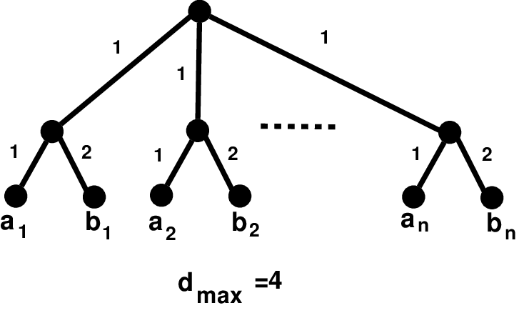
Given a split matching graph with , we associate a caterpillar tree as in Figure 2. The leaves , corresponding to the vertices of , are connected to the spine with edges of weight and the leaves , corresponding to vertices , with edges of weight . It is clear that . Indeed, for any two it holds that , for any two we have and for any we have (hence the edge ) and for any with we have (hence the edge ).∎Note that this representation is not unique. Indeed, one can easily check that the binary tree in Figure 2 also is a pairwise compatibility tree of a split matching graph when .

Lemma 4
Let be a split matching graph. Then .
Proof
Given a split matching graph with , we assume by contradiction . Then let be three leaves of corresponding to three vertices of , . Without loss of generality let be the largest path in the subtree . Consider the vertex in associated to the leaf in , with . From Lemma 1 we deduce that either or . The existence of the edge in implies , therefore one from and must be an edge in , a contradiction. ∎
Analogously, we can show that the set is not empty.
Theorem 3
Let be a split antimatching graph. Then , and in this case it is polynomial to find the tree and the value associated to .
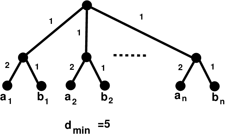
For the sake of brevity we omit the proof of this theorem, that follows using arguments similar to those in the proofs of Lemmas 3 and 4. The tree associated to a split antimatching graph is one from the ones depicted in Figure 3.

4 Split Matrogenic Graphs
In Section 3, when studying the relations among the three classes PCG, LPG and mLPG, we have dealt with threshold graphs, split matchings and split antimatchings. All these graphs are split matrogenic graphs (cfr. definition later). For this reason, it is natural to ask whether split matrogenic graphs are PCG or not. This section is devoted to answer this question.
Definition 2
A split matrogenic graph is the composition of split graphs with such that: either is a split matching or is a split antimatching or (and is called stable graph) or (and is called clique graph).
In order to make easier the exposition, we introduce two subclasses of split matrogenic graphs.
Definition 3
Given a sequence of split graphs with , we say the graph is a split matching (antimatching) sequence if each of the graphs is either a split matching (antimatching), or a stable graph or a clique graph.
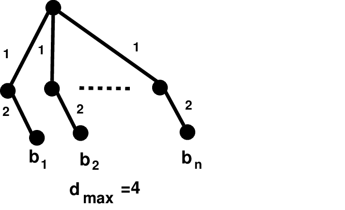
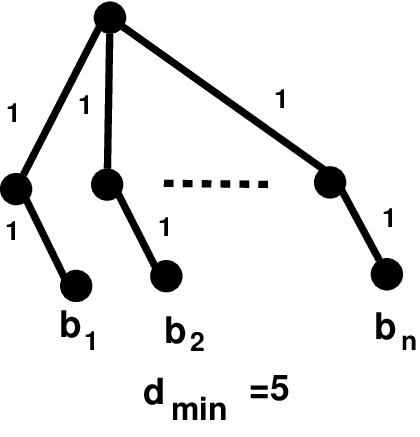
We first prove that split matching sequences and split antimatching sequences are PCG. In both these proofs, in the construction of the pairwise compatibility tree, we will make use of the constructions depicted in Figure 2 and Figure 3, respectively. Finally, we want to point out that a clique graph (a stable graph) can be considered both as a split matching or a split antimatching graph and in each case the pairwise compatibility tree is constructed in the same way, where only leaves (respectively ) appear. In Figure 4 the pairwise compatibility tree is given for a stable graph when it is considered first as a split matching graph and next as a split antimatching graph.
Theorem 4
Let be a split matching sequence. Then and it is polynomial to find the tree and the value associated to .
Proof
Let be a split matching sequence. For each graph we define a tree as shown in Figure 5 (where the leaves () may not possibly appear if is a stable (clique) graph). It is clear that where is a value to be defined later, but surely greater than or equal to . Indeed, let be the leaves of corresponding to vertices of and those corresponding to vertices of . For any two leaves it holds that and for any two we have . Finally, for any two leaves that correspond to an edge of the matching their distance is and for any two leaves corresponding to a non edge their distance is .


In order to prove that , we define a new tree starting from the trees , simply by contracting all their roots to a single vertex as shown in Figure 5. We claim that where we set . In order to prove it, consider two graphs and with . Let and be four distinct leaves corresponding to vertices in and respectively. Observe that the vertices in are connected to all the other vertices in as the distances in are and (as ). Finally, any vertex in is not connected to any vertex and to any vertex as in these cases the distances are (as ) and . ∎
Using similar arguments we prove the following result.
Theorem 5
Let be a split antimatching sequence. Then and it is polynomial to find the tree and the value associated to .
Proof
The proof follows the same lines of the proof of Theorem 4. Let be a split antimatching sequence. We will associate to each split antimatching graph a tree as depicted in Figure 6. We prove that where is a value to be defined later, but surely greater than or equal to . Indeed, let be the leaves of corresponding to vertices of and those corresponding to vertices of . For any two leaves it holds that and for any two we have . Finally, for any two leaves that correspond to an edge of the antimatching their distance is and for any two leaves corresponding to a non edge their distance is .
We define the tree starting from the trees , in the same way we have done in the previous theorem (see Figure 5). Using the same arguments it is not difficult to check that where we have set . Indeed, consider two graphs and with . Let and be four distinct leaves corresponding to vertices in and respectively. Observe that the vertices in are connected to all the other vertices in as the distances in are and . Finally, any vertex in is not connected to any vertex and to any vertex as in these cases the distances are (as ) and . ∎


Theorem 6
Let be a split matrogenic graph such that for any split matching graph and for any split antimatching graph it holds that . Then and it is polynomial to find the tree and the values associated to .
Proof
Let . It is clear that if none of the graphs is a split matching (a split antimatching) the proof trivially follows from Theorem 4 (Theorem 5). Hence, let , , be the first occurrence of a split matching graph. Then, the graphs and are a split matching sequence and a split antimatching sequence, respectively. Then, let where the tree is constructed in the same way as in the proof of Theorem 4 and (recall that in the proof of Theorem 4 we only need to be a value greater that ). Similarly, according to the Theorem 5, and (note that we choose to have )). We modify in such a way that of the weights of the edges outcoming form the root start from value instead of from and the other edges are modified accordingly. This is not restrictive, as results as if was the composition of split antimatching graphs whose the first are empty graphs.
We construct the pairwise compatibility tree by joining the roots of and with an edge of weight . We set and . We modify the weights of the resulting tree increasing by the weight of any edge incident to a leaf in . Observe that in this way the distance of any two leaves in is increased by . This means that two leaves correspond to vertices of an edge in if and only if their distance is less than or equal to . Furthermore, the maximum distance of any two leaves in is less than or equal to meaning that they correspond to vertices of an edge in if and only if their distance is greater than or equal to .
We claim that (recall that ). We have already shown that the pairwise compatibility constraints hold for any two leaves that correspond to two vertices of the same graph or . It remains to show it also holds for two leaves where one corresponds to a vertex in and the other to . To this purpose, let and be two distinct leaves in , connected to the root with edges of weight and corresponding to vertices of the clique and the stable graph of , respectively. Similarly let be two distinct leaves in , connected to the root with edges of weight and corresponding to vertices in the clique and the stable graph of , respectively. The following hold:
- a)
and as and then . Hence, the corresponding vertices of in are connected.
- b)
and as then . Hence, the corresponding vertices of in are connected.
- c)
and as then . Hence, the corresponding vertices of in are not connected.
- d)
and as then . Hence, the corresponding vertices of in are not connected.
This, concludes the proof. ∎
It seems that the order of appearance of a matching or an antimatching sequence in a split matrogenic graph is somehow strictly related to the pairwise compatibility property. Indeed, in spite our efforts, the following problem remains open.
Problem: Let be a split matrogenic graph such that for any split antimatching graph and for any split matching graph it holds that . Is a PCG ?
If this problem has an affermative answer then it should not be difficult to prove that all split matrogenic graphs are PCG. Otherwise, the separation between the split matrogenic graphs that are PCG and those that are not, would be perfectly known.
5 Conclusions and Open Problems
In this paper we analyze the class of PCG with particular attention to two particular subclasses resulting when the pairwise compatibility constriants are relaxed. Hence, we consider the sublasses LPG and mLPG, resulting from the the cases where and , respectively. We study the relations between the classes PCG, LPG and mLPG. In particular, we show that the union of LPG and mLPG does not coincide with the whole class PCG, their intersection is not empty, and that neither of the classes LPG and mLPG is contained in the other. The graphs considered in these considerations are particular cases of the more general class of split matrogenic graphs. Hence, we attempt to determine whether the class of split matrogenic graphs belongs to PCG class. We prove that many split matrogenic graphs are PCG. However, the membership to PCG class of one particular split matrogenic graph remains an open problem.
It should be stressed that up to date, the pairwise compatibility has been investigated only for a few classes of graphs, thus determine this property for many graph classes remains an open problem. It is worth to mention that in [3] is shown that the clique problem can be solved in polynomial time for the class of compatibility graphs if we are able to construct in polynomial time a weighed tree that generates the pairwise compatibility graph. In view of this, it seems even more interesting to completely identify the Pairwise Compatibility graphs class.
References
- [2] A. Brandstädt. : On Leaf Powers. Technical report, University of Rostock, (2010).
- [3] P.E. Kearney, J. I. Munro and D. Phillips: Efficient generation of uniform samples from phylogenetic trees. In: Benson, G., Page, R.D.M. (eds.) WABI. Lecture Notes in Computer Science, vol. 2812, pp. 177–189. Springer, Berlin (2003).
- [4] N. Nishimura, P. Ragde, D.M. Thilikos, On graph powers for leaf-labeled trees, J. Algorithms 42 (2002) 69-108.
- [5] Phillips, D.: Uniform sampling from phylogenetics trees. Masters Thesis, University of Waterloo (2002).
- [6] Nur Yanhaona, M., Bayzid, Md.S., Rahman, Md. S.: Discovering Pairwise compatibility graphs. J. Appl. Math. Comput. 30, 479–503 (2009).
- [7] Nur Yanhaona, M., Hossain, K.S.M. T. Rahman, M. S.: Pairwise compatibility graphs. J. Appl. Math. Comput. 30, 479–503 (2009).