Parton showers as sources of energy-momentum deposition in the QGP and their implication for shockwave formation at RHIC and at the LHC
Abstract
We derive the distribution of energy and momentum transmitted from a primary fast parton and its medium-induced bremsstrahlung gluons to a thermalized quark-gluon plasma. Our calculation takes into account the important and thus far neglected effects of quantum interference between the resulting color currents. We use our result to obtain the rate at which energy is absorbed by the medium as a function of time and find that the rate is modified by the quantum interference between the primary parton and secondary gluons. This Landau-Pomeranchuk-Migdal type interference persists for time scales relevant to heavy ion phenomenology. We further couple the newly derived source of energy and momentum deposition to linearized hydrodynamics to obtain the bulk medium response to realistic parton propagation and splitting in the quark-gluon plasma. We find that because of the characteristic large angle in-medium gluon emission and the multiple sources of energy deposition in a parton shower, formation of well defined Mach cones by energetic jets in heavy ion reactions is not likely.
1 Introduction
The suppression in the production rates of energetic leading particles and jets in relativistic heavy ion reactions relative to a naive superposition of nucleon-nucleon collisions is one of the most striking results from the heavy ion program at the Relativistic Heavy Ion Collider (RHIC) [1] and now at the Large Hadron Collider (LHC) [2, 3]. These phenomena, often collectively referred to as “jet quenching” [4], have been studied extensively both experimentally and theoretically and are thought to provide valuable information about the quark-gluon plasma (QGP) created in these events [5].
At a fundamental level, the physics of jet quenching is largely reflective of the interaction of energetic, or fast, partons with the QGP medium which they traverse. Fast partons lose energy primarily through medium-induced radiation [6]. Thus, the original fast parton evolves into an in-medium parton shower. The shape and energy distribution associated with this shower provide more information about the underlying QCD dynamics than the suppression of leading particles alone and form the basis for using full jet observables as a new and powerful probe of the QGP [7].
Parton showers can also be substantially modified through collisional energy losses to the underlying medium. Although the collisional energy loss associated with a single parton is thought to be relatively small, the cumulative effect associated with a full parton shower can become quite large as the radiated gluons themselves become sources of collisional energy loss. Thus, the question of how much energy a parton shower transmits to the medium is of fundamental interest in the description of full jet observables.
A closey related question is how the medium responds to a parton shower. As a parton shower loses energy and momentum, the underlying medium is affected in a way that depends on its properties as well as the space-time distribution of the energy and momentum deposition. This problem has gained attention due to experimental measurements of azimuthal particle correlations associated with high triggers in heavy ion collisions that display a double-peaked or conical structure [8]. These measurements may reflect the interaction of fast partons with the medium and among the proposed explanations for the structure are Mach cone shockwaves excited in the bulk medium by fast partons [9]. Other explanations that do not reflect the interaction of fast partons with the medium, such as fluctuating initial conditions and triangular flow have also been proposed [10]. Whether or not the conical structure associated with high triggers at RHIC is associated with the medium response to a parton shower, this topic remains important, particularly in the light of the the new exciting possibilities for jet physics with the LHC heavy ion program.
Both the question of how much energy a parton shower transmits to the medium and how the medium responds to a parton shower can be addressed in the same framework by calculating the source term associated with the parton shower. The source term, here denoted , is the space-time distribution of energy and momentum flowing between a parton shower and the underlying medium. It couples to the energy-momentum tensor (EMT) as . The source term carries information about the rate of energy transfer to the medium and acts as a source (hence the name “source term”) for the evolution of the underlying medium in the presence of the parton shower.
Previous calculations of the source term have focused on a single primary parton [11]. Applications to shockwave formation that have attempted to include medium-induced gluon bremsstrahlung have neglected the spatial extent of the source and, just as importantly, the color quantum interference between the primary parton and associated radiation [12]. In what follows we will perform the first calculation of the source term associated with a parton shower. Our calculation will include the full spatial extent and color quantum interference effects, and will be presented in closed analytic form. To perform this calculation, we will start with the result of a recent paper by Neufeld [13] in which the source term induced by a single fast parton in a medium of thermal quarks was derived in integral form using thermal field theory. The source term was obtained by taking the thermal average of the divergence of the quark energy-momentum tensor, with the fast parton coupled to the medium by adding an interaction term to the Lagrangian.
Our paper is organized as follows: we present the theoretical formalism for the evaluation of the source term associated with a parton shower in section 2. In section 3 we present two applications of the source term we derive: the rate of energy transfer between the parton shower and the medium and the response of the medium to the parton shower. We show that a significant amount of energy can be transferred from the parton shower to the medium depending sensitively on the average angle of gluon radiation. We further show that for realistic average angle of gluon emission the medium response no longer appears as a well defined Mach cone but rather a superposition of several distinct perturbations in the medium. Our summary and conclusions are given in section 4.
2 Theoretical formalism
Our approach in this section is to extend the result presented in [13] to the case of an asymptotically propagating primary fast parton which undergoes medium-induced gluon bremsstrahlung. In this manuscript we use the following 4-vector notation: .


Our starting points are the Feynman diagrams of Figure 1. The dark blobs represent the divergence of the medium energy-momentum tensor, for which we will implement the result derived in [13]. In the left diagram of Figure 1 the gluon lines labeled with and connect the medium to the primary fast parton (a quark in the diagram), in the middle diagram they connect to the radiated gluon, and in the right diagram they connect to both. This diagram represents the non-trivial quantum interference between the two partons. A fourth diagram with and exchanged in the interference term is not shown in Figure 1 but is included in the calculation presented here.
In Figure 1 the SU(3) color matrices are denoted by upper and lower case and for the adjoint and fundamental representations, respectively. Using standard color algebra, we find that the color factors for the first two diagrams in Figure 1 simply yield the quadratic Casimir of the particular representation: for a quark (first diagram) and for a gluon (middle diagram). The color factors for the third and fourth (not shown) diagrams yield each. We point out that the color factors of these last two contributions remain the same if the primary parton is a gluon. Note that we have averaged over the initial colors and factored out the Casimir associated with the bremsstrahlung vertex.
If for the moment we write the divergence of the medium EMT as an arbitrary function (with and being the velocity 4-vectors of the primary parton and radiated gluon, respectively), then the combined result for the four contributing diagrams is:
| (1) | |||||
where is the quadratic Casimir of the primary parton and the subscript indicates that we consider the primary parton to propagate asymptotically. In the limit of perfectly collinear radiation one has and the interference terms exactly cancel the contribution from the radiated gluon. This result reflects the fact that the medium will never resolve the bremsstrahlung gluon from the parent parton and the color of the system is the same before and after the radiation. However, if radiation is not perfectly collinear (and ), the system evolves in time, the two new color currents separate, and the interference terms gradually vanish. At the system begins to look like two separate color charges.
In this work we consider the primary parton to be propagating asymptotically, that is we ignore any finite time effects associated with the initial large scattering in a heavy ion collision. This problem has been examined in a different context in [14]. Although these effects are important to understand and may very well be significant, our focus is instead on the time dependence associated with the gluon radiation and the interference effects that arise with it. When both gluon lines attach to the primary quark, the current can be represented by the classical asymptotic form: with . Similarly, when both gluon lines attach to the secondary gluon the current can be represented by the form . However, when the gluon lines are connected as in the third diagram of Figure 1 there is no simple way to express the current and one must combine the product. The result is reflected in Eq. (1): , where we only consider interference effects after the point of emission.
With these considerations in place, we write the integral expression for the source term derived in [13] for an asymptotically propagating fast parton in a medium of thermal quarks, corresponding to the first diagram of Figure 1 and written in the notation of Eq. (1):
| (2) |
where is the retarded Green’s function, is the Fermi distribution function, is the temperature, and is the number of active flavors.
For our calculation we also need the generalization of Eq. (2) to the case of two separate velocities, that is , created at an initial time . The primary effect of this modification enters through the function structure of Eq. (2):
| (3) |
The above replacement can easily be understood from the integral representation of the function: . For the case of a charge created at time the integration begins at 0 rather than . One can see that after contour integration in the variables the primary result of the replacement made in Eq. (3) is that and no longer enter the exponential symmetrically when . The result is that the contribution from will die out on an timescale related to the inverse of the difference between and .
The specific generalization of the polynomial structure in the numerator (the third and fourth lines) of Eq. (2) to the case of two separate velocities is not as essential as the replacement shown in Eq. (3) (or the pole structure). In particular, corrections to the form of Eq. (2) are at most proportional to , which should be suppressed when the radiation angle is smaller than one. With this in mind, we make the obvious assignment that the first term remain symmetric in . For the second term we use the form:
| (4) |
based on the relation of and in the Green’s function structure. In the worst case, the correction in this second term is proportional to . The combined result can be written as:
| (5) |
The full source term, which is the sum of the terms in Eq. (1), can now be obtained by evaluating the expressions given in Eqs. (2) and (5). As we will show in what follows, one actually only needs to evaluate Eq. (5), for which Eq. (2) can be obtained as a special case.
We now proceed to evaluate Eq. (5). In order to simplify the calculation we use bare propagators and take the hard thermal loop (HTL) approximation. These simplifications will allow us to obtain an analytic result for the source term. We also will consistently ignore radiative effects arising from the formation of a charge at an initial time. These effects are associated with causality and are in addition to the medium induced radiation we are considering in this paper. We postpone their consideration to a future work. We emphasize that all vacuum contributions have already been subtracted from Eq. (5). Furthermore, although (5) was derived for a medium of quarks (as can be seen from the number of active flavors and the Fermi distribution ) the extension to include medium gluons is trivial in the HTL limit as will be shown below.
We obtain the HTL approximation by taking the limit that the fields generated by the external current are soft compared to the temperature, or formally in Eq. (5). The coupling constant is formally considered to be much less than one. Explicitly, we expand in the limit of since , which appears in the Fermi distribution function, is cut off in the integration at a value on the order of to lowest contributing order. We find that in the HTL approximation Eq. (5) reduces to:
| (6) | |||||
where for a thermal medium comprised quarks only. In Eq. (6) is the integration measure over the solid angle defined by the unit vector , and . As mentioned previously, the extension to include medium gluons is straightforward and is done with the modification .
In order to evaluate Eq. (6) it is convenient to note that the and integrations separate. The contribution has the same general form in each term which we evaluate as:
| (7) |
where , , and we ignore radiative effects on the light cone associated with the formation of the field. The result of Eq. (7) can be derived in a straightforward manner by expressing components of as a derivative on and using the relationship that along with . The step function in Eq. (7) is a result of causality and ensures that the final result for the source term will only contribute in the time-like region.
The integration in Eq. (6) cannot be separated from the integration and thus is more involved. For the first term one is aided by the cancellation occurring from . Again using and writing followed by an integration by parts allows:
| (8) |
where . At this point the integration is performed to yield a function, which enables the remaining integrals to be performed analytically. The result is obtained as
| (9) |
where
| (10) |
Lastly, we must evaluate:
| (11) |
The first term in Eq. (11) can be obtained in the same manner as Eq. (7) with the result:
| (12) |
The second term is more involved and for the sake of brevity we briefly outline the important steps in obtaining the result. We first write and then use contour methods to perform the integration (which places a restriction that ). One can next perform the integration to leave:
| (13) |
The second line of Eq. (13) can be simplified by redefining the angular variable in terms of : that is, let , where is associated with . One can further use the relations and to reduce the expression to two integrals which can be performed in closed form using standard integral relations. The result is:
| (14) |
where for simplicity we have restricted our attention to the region of knowing from Eq. (7) that this is the only region that contributes in the final expression.
Finally we consider the third line of Eq. (13), which can again be simplified by redefining the angular variable in terms of . One can further use the integral relations and [15]:
| (15) | |||
| (16) |
to again reduce the expression to two integrals. In the above expressions are Bessel functions of the first kind, and is a positive infinitesimal quantity. Performing the final two integrations, we find
| (17) |
We now have all of the necessary pieces to yield a final result for Eq. (6). In order to achieve a compact form, is it helpful to define the notation , in which case one finds:
| (18) |
where we have defined . Equation (18) is our primary result and we now discuss its general features and also how to specialize it to the asymptotic case . Eq. (18) is restricted by causality, which is contained in the step function . Furthermore, the first four lines of Eq. (18) contribute in the asymptotic limit, whereas the last two lines are transient contributions, that is, they vanish as even for . This can be seen by taking the case of and allowing , while taking . Thus one can obtain the asymptotic case by removing the step function and the final two lines of Eq. (18), and of course setting . In this asymptotic limit our result should reduce to the result obtained previously by Neufeld in [11]. We have verified numerically that this is indeed true.
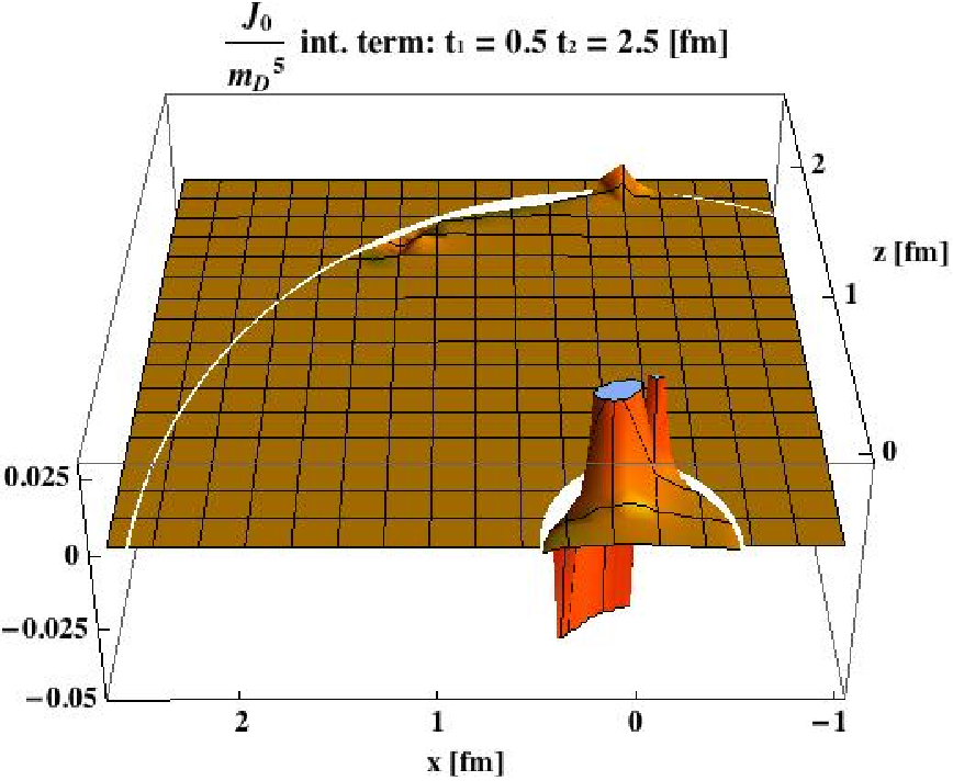
Recall from Eq. (1) that the total source term is given by the combination , where the last two terms result from the interference graphs of Figure 1 and we refer to this contribution as “interference term” in what follows. To help illustrate the result of Eq. (18) we plot the interference term contribution for two different times in Figure 2 above. For all numerical results we use the following parameters: , GeV and , which are based on the average values obtained for LHC collision energies in a Bjorken expanding plasma and we take for a gluon-dominated medium. Additionally we impose medium-induced Debye screening through an exponential decay factor, , where and are distances transverse to the axes of propagation defined by and , respectively. The velocity of the primary parton is chosen along the axis with a magnitude determined by the energy and mass of the parton: with for a quark and for a gluon. The magnitude of the velocity of the radiated gluon is determined in the same way as the primary parton, and its direction determined by the angle of emission relative to the direction of the primary parton’s propagation. For simplicity we will take the emission to occur in the plane unless otherwise stated. Thus, all quantities are determined by specifying the energies of the primary parton and the radiated gluon, as well as the angle of emission.


We plot the interference term contribution for two different times in Figure 2 above. For this plot we choose a primary quark with energy Gev, a radiated gluon with energy GeV and angle of emission (angles will always be given in radians). Although these energies are phenomenologically small, they are convenient for the purposes of plotting. The plot shows the zero component of the interference term contribution scaled to a dimensionless ratio for times fm and fm (in the same figure), where time is measured from the moment of emission. The plot shows that at early times when the two partons are close together their interference contribution is important, but at later times as they become separated the interference contribution diminishes and eventually vanishes. In the next section we consider two applications of the source term derived in Eq. (18).
3 Applications: differential energy transfer to the medium and linearized hydrodynamics
The main theoretical result of this paper is Eq. (18), which combined with Eq. (1) gives the source term for a primary parton and a single radiated gluon as a function of time, including quantum color interference effects. In this section, we consider two applications of our result: the evaluation of the differential energy lost by a parton shower to the medium and the hydrodynamic response of the medium to a parton shower.
The differential energy transfer to the medium is obtained from the source term through a spatial integration of the zero component:
| (19) | |||||
This transfer is of a collisional nature and the terms involving only one velocity, and , are fraught with an ultraviolet divergence typical of collisional energy loss [16]. We regulate these terms with a standard short distance cutoff related to the finite momentum transfer, where is the distance transverse to the axis of propagation defined by and is the corresponding energy. On the other hand, the terms involving two velocities, and , have no ultraviolet divergence and require no cutoff. However, motivated by the finite kinematics and for consistency, we apply a short distance cutoff to these terms reflective of two distinct gluon exchanges: . As these terms have no ultraviolet divergence, the sensitivity to the cutoff for the interference contribution is small.


We now consider two scenarios for the differential energy transfer to the medium which are both presented in Figure 3. The first is shown in the left panel and is for a primary quark of energy 75 GeV which emits a gluon of energy 4.5 GeV at time fm. At this point the primary quark’s energy is reduced to 70.5 GeV. The differential energy loss to the QGP is shown for three different angles of emission, as well as without any interference effects. It should be noted that even in the absence of interference it takes on the order of for the radiative gluon to build up its asymptotic energy transfer rate (see the solid curve). The strength of interference effects depends on the transverse separation of the two color currents. When these currents cannot be resolved by the medium the system behaves like the parent parton. This is illustrated by the smallest emission angle we consider, . The red dashed curve shows the fact that interference suppresses the energy loss to the medium for times extending up to about 3-4 fm after emission. For the larger angle of there is a slight suppression initially followed by a slight enhancement persisting until about 2 fm after emission. Finally, we also consider as we are motivated by the finding that the medium-induced bremsstrahlung is dominated by large angles [17]. For this largest angle the energy loss actually shows an enhancement relative to no interference which persists for about 2 fm after emission. The insert shows the total energy transferred to the medium for the different angles as a function of time.
Next, we consider a more realistic representation of the medium-induced parton shower inspired by the Gyulassy-Levai-Vitev (GLV) energy loss formalism [18]. Such parton showering is relevant to phenomenological applications that aim to elucidate the medium response to jet propagation in hot and dense QCD matter [19]. Specifically, we make use of the bremsstrahlung spectra for quark and gluon jets averaged over the collision geometry in central Pb+Pb reactions at the LHC that have been previously employed to discuss jet and particle production in heavy ion collisions at the highest [20]. Medium-induced gluon emission is probabilistic and depends on the parton species. The most likely numbers are 4 ( GeV) and 8 ( GeV) for 75 GeV quark and gluon parent partons, respectively. We also note that the average emission angle is quite large, . The gluon emission points are uniformly distributed along the parton propagation path in a medium of length 5 fm. In the GLV approach the gluon distribution is azimuthally symmetric around the direction of jet propagation. For simplicity, we distribute them here in the x-z plane. Further, quantum interference effects are only taken between the primary parton and each radiated gluon - not between the multiple radiated gluons. The result is shown in the right panel of Figure 3 where again we find an enhancement of energy transfer to the medium. The insert shows the total energy transferred to the medium where one sees that for a gluon-induced shower its value is about 32 GeV for our parameters.
We now evaluate the hydrodynamic response of the medium to a parton shower. We consider the realistic scenario discussed directly above, only we now include both and . By comparing these two angles we can illustrate clearly the effect of the interference on the medium response. The implementation of the full source term is rather numerically expensive therefore in this exploratory study we implement the simplest possible description of the shower by treating each parton as a function source with a weight given by the energy loss rate to the medium: , where the subscript refers to a summation over each parton in the shower. This simplified form of the source correctly accounts for energy and momentum conservation and allows us to incorporate the energy loss rates evaluated above. We make the stipulation that the contribution coming from the quantum interference is associated with the radiated gluon rather than the primary quark.
We focus on the energy density perturbation, , generated in the medium by the parton shower. Within linearized hydrodynamics this quantity can be written in momentum space as [21]
| (20) |
In the above equation, denotes the speed of sound and is the sound attenuation length with being the shear viscosity to entropy density ratio in the medium. Also, the source vector has been divided into transverse and longitudinal parts: . In addition to the parameters listed above we choose the proposed minimum bound for the shear viscosity to entropy density ratio [22]. Although shear viscosity estimates obtained from phenomenological studies of hydrodynamic simulations of the bulk matter produced in heavy ion experiments [23] suggest a value perhaps 2-3 times larger than , we have chosen the minimum bound because it is particularly well suited for plotting the important features of the medium response.
In Figure 4 we present the result for for the scenario and parameters discussed above. We consider a primary quark of energy 75 GeV which emits 4 gluons of energy 4.5 GeV. The gluon emissions are uniformly distributed over the primary quark’s path length of 5 fm, at which point we plot the medium response. For the purpose of illustration we have chosen the gluon emissions to alternate between the positive and negative directions, although in practice they are randomly distributed in the plane. Additionally, we have scaled the energy density distributions associated with each parton by a factor of to compensate for the broadening of the Mach cones. Here, and are the initial position and time of the particular parton.
In the left and right panels of Figure 4 we show the result for and , respectively. One can see that for the narrow emission angle the parton shower generates a well defined Mach cone similar to what one would expect from a single primary parton [24]. However, the interference effects from such small angle emissions suppress the energy transfer such that the total energy gained by the medium is only moderately enhanced compared to the single primary parton (about 1.7 times larger for our parameters). Contrast this to previous studies which ignored the interference suppression and found significant enhancement even for exactly collinear radiation [12]. For the larger emission angle there is no longer a well defined Mach cone but rather a superposition of several distinct perturbations in the medium. The interference effects for this angle actually lead to an enhancement in the overall energy gained by the medium, even relative to no interference. Compared to the single primary parton the energy gain is about 2.7 times larger. However, the price for this gain in energy is that there is no longer a well defined Mach cone structure.
4 Conclusions
In this Letter we evaluated the source term of energy and momentum deposited by a parton shower in the QGP in closed analytic form. Our result includes for the first time the quantum interference effects between the color currents associated with the primary parton and the radiated gluon. We demonstrated that the interference term that spoils the naive classical superposition [12] of incoherent energy and momentum transfer rates persists for time scales relevant for heavy ion phenomenology. We showed that this term vanishes in the limit, as it must.
We presented two applications of the source term derived in this paper: the evaluation of the differential rate of energy transfer by a parton shower to the medium and the hydrodynamic response of the medium to a parton shower. The former should not be confused with the rate of collisional energy loss [14] of the parent parton itself, which remains constant and relatively small. We found that the rate of energy and and momentum transfer from the parton shower to the medium depends sensitively on the angle of emission and number of gluons emitted. For collinear bremsstrahlung, the medium cannot resolve the primary parton and the radiated gluon and there is pronounced coherent suppression in the magnitude of the multi-parton source term. For realistic large angles of emission [17], we actually find an enhancement in its amplitude. Using the GLV formalism to describe the medium-induced parton shower [18], including bremsstrahlung gluon multiplicities, energies and emission angles, we estimated that for LHC applications [20] a 100 GeV parton can transmit more than 1/3 of its energy to the QGP. In the future, we plan to conduct more detailed numerical simulations that include realistic geometry and expansion of the medium and improved calculations of parton shower formation in the QGP [25]. We note, however, that our findings suggest that the rate of jet energy dissipation in the medium may significantly complicate the experimental/jet medium background separation at RHIC and at the LHC [2, 26].
We embeded the newly-derived source term in linearized hydrodynamics to study the response of the QGP to the in-medium parton shower. We found that for small gluon emission angles and minimal shear viscosity to entropy density ratio [22] the parton shower generates a well defined Mach cone similar to what one would expect from a single primary parton or from a phenomenological incoherent collinear superposition of a parton with gluons [12]. For realistic multiple gluon emission at large angles [17] there is an enhancement in the rate of energy transfer to the medium not only from the development of the parton shower but also from the interference effects discussed in this Letter. This, in turn, yields a larger perturbation of the energy density in the medium but there is no longer a well defined Mach cone in the QGP. Our result is intuitive and easy to understand: each parton in the developing shower gradually becomes a separate source of energy deposition and excitation of the strongly-interacting medium. The overlapping perturbations in very different spatial directions wipe out any distinct Mach cone structure. Our finding is critical for heavy ion experiments and phenomenology. It suggests that schematic treatments of the parton shower provide an inaccurate description of shockwave phenomena in the QGP. It also suggests that high triggers are not likely to have well defined away-side associated shockwave structures, since the number of medium-induced gluons grows with the parent parton energy [18].
References
- [1] K. Adcox et al., Phys. Rev. Lett. 88, 022301 (2002); C. Adler et al., Phys. Rev. Lett. 89, 202301 (2002).
- [2] S. Chatrchyan et al. [ CMS Collaboration ], [arXiv:1102.1957 [nucl-ex]];
- [3] K. Aamodt et al. [ ALICE Collaboration ], Phys. Lett. B696, 30-39 (2011).
- [4] M. Gyulassy, I. Vitev, X. N. Wang and B. W. Zhang, arXiv:nucl-th/0302077.
- [5] I. Arsene et al., Nucl. Phys. A 757, 1 (2005); B. B. Back et al., Nucl. Phys. A 757, 28 (2005); J. Adams et al., Nucl. Phys. A 757, 102 (2005); K. Adcox et al., Nucl. Phys. A 757, 184 (2005).
- [6] M. Gyulassy and X. N. Wang, Nucl. Phys. B 420, (1994) 583; R. Baier, Y. L. Dokshitzer, A. H. Mueller, S. Peigne and D. Schiff, Nucl. Phys. B 484, (1997) 265; B. G. Zakharov, JETP Lett. 65, (1997) 615; U. A. Wiedemann, Nucl. Phys. B 588, (2000) 303; M. Gyulassy, P. Levai and I. Vitev, Nucl. Phys. B 594, (2001) 371;
- [7] I. Vitev, S. Wicks, B. -W. Zhang, JHEP 0811, 093 (2008); I. Vitev, B. -W. Zhang, Phys. Rev. Lett. 104, 132001 (2010); T. Renk, Phys. Rev. C80, 044904 (2009).
- [8] J. Adams et al., Phys. Rev. Lett. 95, 152301 (2005); S. S. Adler et al., Phys. Rev. Lett. 97, 052301 (2006); B. I. Abelev et al., Phys. Rev. Lett. 102, 052302 (2009); A. Adare et al., Phys. Rev. C 78, 014901 (2008).
- [9] J. Casalderrey-Solana, E. V. Shuryak and D. Teaney, J. Phys. Conf. Ser. 27, 22 (2005). L. M. Satarov, H. Stöcker and I. N. Mishustin, Phys. Lett. B 627 (2005) 64.
- [10] B. Alver, G. Roland, Phys. Rev. C81, 054905 (2010).
- [11] R. B. Neufeld, Phys. Rev. D78, 085015 (2008).
- [12] R. B. Neufeld, B. Muller, Phys. Rev. Lett. 103, 042301 (2009). G. -Y. Qin, A. Majumder, H. Song, U. Heinz, Phys. Rev. Lett. 103, 152303 (2009).
- [13] R. B. Neufeld, Phys. Rev. D83, 065012 (2011).
- [14] P. -B. Gossiaux, S. Peigne, C. Brandt, J. Aichelin, JHEP 0704, 012 (2007); A. Adil, M. Gyulassy, W. A. Horowitz, S. Wicks, Phys. Rev. C75, 044906 (2007).
- [15] A. Erdelyi, W. Magnus, F. Oberhettinger and F.G. Tricomi, Tables of Integral Transforms, Vol. 1, New York, McGraw-Hill (1954).
- [16] M. H. Thoma, Phys. Lett. B 273, 128 (1991).
- [17] I. Vitev, Phys. Lett. B630, 78-84 (2005).
- [18] I. Vitev, Phys. Rev. C75, 064906 (2007).
- [19] A. K. Chaudhuri and U. Heinz, Phys. Rev. Lett. 97, 062301 (2006); T. Renk and J. Ruppert, Phys. Rev. C 73 (2006) 011901; B. Betz, M. Gyulassy, J. Noronha and G. Torrieri, Phys. Lett. B 675, 340 (2009). H. Li, F. Liu, G. -l. Ma, X. -N. Wang, Y. Zhu, Phys. Rev. Lett. 106, 012301 (2011); I. Bouras, A. El, O. Fochler, F. Reining, J. Uphoff, C. Wesp, Z. Xu, C. Greiner, [arXiv:1102.2518 [hep-ph]].
- [20] R. Sharma, I. Vitev, B.-W. Zhang, Phys. Rev. C80, 054902 (2009); R. B. Neufeld, I. Vitev, B.-W. Zhang, Phys. Rev. C83, 034902 (2011); Z.-B. Kang, I. Vitev, in preparation; Rishi Sharma, I. Vitev, in preparation; Y. He, I. Vitev, B.-W. Zhang in preparation.
- [21] R. B. Neufeld, T. Renk, Phys. Rev. C82, 044903 (2010).
- [22] P. Kovtun, D. T. Son and A. O. Starinets, Phys. Rev. Lett. 94, 111601 (2005).
- [23] P. Romatschke and U. Romatschke, Phys. Rev. Lett. 99, 172301 (2007).
- [24] R. B. Neufeld, B. Muller, J. Ruppert, Phys. Rev. C78, 041901 (2008).
- [25] G. Ovanesyan, I. Vitev, [arXiv:1103.1074 [hep-ph]].
- [26] G. Aad et al. [ Atlas Collaboration ], Phys. Rev. Lett. 105, 252303 (2010).